Magnetic properties of the extended periodic Anderson model

Abstract

We study magnetic properties of the extended periodic Anderson model, which includes electron correlations within and between itinerant and localized bands. By combining dynamical mean-field theory with the numerical renormalization group we calculate the sublattice magnetization and the staggered susceptibility to determine the phase diagram in the particle-hole symmetric case. We find that two kinds of magnetically ordered states compete with the Kondo insulating state at zero temperature, which induces non-monotonic behavior in the temperature-dependent magnetization. It is furthermore clarified that a novel magnetic metallic state is stabilized at half filling by the competition between Hund’s coupling and the hybridization.

Strongly correlated electron systems with degenerate orbitals have attracted great interest. One of the popular examples is the manganite $\rm(La,Sr)MnO_{3}$.[1] In this system, itinerant electrons in the $e_{g}$ band are coupled to localized electrons in the $t_{2g}$ band through Hund’s coupling, leading to a competition between antiferromagnetic (AF) correlations and the double exchange ferromagnetic correlations. This yields a complex phase diagram with various types of ordered ground states. Other interesting examples are $\rm(Ca,Sr)_{2}RuO_{4}$[2] and $\rm La_{n+1}Ni_{n}O_{3n+1}$.[3, 4] In these compounds, the chemical substitution or the change in temperature is suggested to trigger an orbital-selective Mott transition,[5, 6] where some of the orbitals become localized by electron correlations, while the others still remain itinerant. It is also proposed that in these compounds, localized and itinerant electrons are hybridized with each other, inducing heavy fermion or bad metal behavior at low temperatures.[7, 8, 9, 10]

An important point in the above compounds is that the localized and itinerant bands in the $d$-orbital and their correlations play a crucial role in stabilizing the magnetically ordered state or heavy fermion state. Generally speaking, in the systems with localized bands, the hybridization together with local electron correlations screen spins, leading to heavy fermion behavior with the large density of states (DOS) around the Fermi level, the so-called Kondo effect. [12, 11, 13] In contrast, Hund’s coupling enforces parallel spins in different orbitals, enhancing magnetic correlations, as discussed for the manganites.[14, 15, 16, 17] Therefore, an interesting question arises how robust the nonmagnetic ground state is in systems with localized and itinerant bands. In a previous paper,[9] we have investigated the extended periodic Anderson model (EPAM) to clarify how the Kondo and Mott insulating states compete with the metallic state in the paramagnetic case. However, a magnetic instability has not been discussed so far, which may be important to understand low-temperature properties in real materials such as some transition metal oxides and $f$-electron systems. Furthermore, the competing interactions may lead to nontrivial behavior in the magnetically ordered state. Therefore, it is highly desirable to clarify the magnetic properties in the system with localized and itinerant electrons.

For this purpose, we consider a correlated electron system which is described by the following Hamiltonian as,

$${\cal H} = H_{t}+\sum_{i}H_{loc}^{(i)},$$ (1)

$$H_{t} = \sum_{\langle ij\rangle\alpha\sigma}\left[t_{ij}^{(\alpha)}-\mu\delta_{ij}\right]c_{i\alpha\sigma}^{\dagger}c_{j\alpha\sigma},$$

$$H_{loc}^{(i)} = V\sum_{\sigma}\left(c_{i1\sigma}^{\dagger}c_{i2\sigma}+c_{i2\sigma}^{\dagger}c_{i1\sigma}\right)$$

$$+ \sum_{\alpha}U_{\alpha}n_{i\alpha\uparrow}n_{i\alpha\downarrow}+\sum_{\sigma\sigma^{\prime}}\left(U^{\prime}-J\delta_{\sigma\sigma^{\prime}}\right)n_{i1\sigma}n_{i2\sigma^{\prime}}$$

$$- J\sum_{\sigma}c_{i1\sigma}^{\dagger}c_{i1\bar{\sigma}}c_{i2\bar{\sigma}}^{\dagger}c_{i2\sigma}-J\sum_{\alpha}c_{i\alpha\uparrow}^{\dagger}c_{i\alpha\downarrow}^{\dagger}c_{i\bar{\alpha}\uparrow}c_{i\bar{\alpha}\downarrow},$$

where $c_{i\alpha\sigma}^{\dagger}(c_{i\alpha\sigma})$ creates (annihilates) an electron with spin $\sigma(=\uparrow,\downarrow)$ and band index $\alpha(=1,2)$ at the $i$th site, and $n_{i\alpha\sigma}=c_{i\alpha\sigma}^{\dagger}c_{i\alpha\sigma}$. For the band $\alpha$, $t_{ij}^{(\alpha)}$ represents the transfer integral, $V$ the hybridization between bands. The intra-band and inter-band Coulomb interactions are described by $U_{\alpha}$ and $U^{\prime}$, while $J$ denotes Hund’s coupling. Finally, $\mu$ is the chemical potential.

To investigate the correlated electron system with one band localized and the other itinerant, we set the hopping integral for the $\alpha=2$ band to $t_{ij}^{(2)}=0$, for simplicity. Then this model is regarded as the EPAM with not only intraband interactions but also interband ones. Here, to discuss magnetic properties, we make use of dynamical mean-field theory (DMFT).[18, 19, 20, 21] In DMFT, a lattice model is mapped to an effective quantum impurity, where local electronic correlations are taken into account exactly. The requirement that the site-diagonal lattice Green function is equal to that of the effective quantum impurity then leads to a self-consistency condition for the parameters entering the impurity problem. This treatment is formally exact in infinite spatial dimensions and even for three dimensions reliable results are obtained if non-local correlations are allowed to be ignored.

When an AF instability is treated in the framework of DMFT,[22, 24, 23, 25] the self-consistency equation for the sublattice $\gamma[=(A,B)]$ is represented as,

$$\left[\hat{\cal G}_{0\;\gamma\;\sigma}^{-1}(z)\right]_{11}=z+\mu-\left(\frac{D}{2}\right)^{2}\left[\hat{G}_{loc\;\bar{\gamma}\;\sigma}(z)\right]_{11},$$ (2)

where $\hat{\cal G}_{0}$ is the non-interacting Green function for the effective impurity model and $\hat{G}_{loc}$ the local Green function. Here, we have used the Bethe lattice with infinite coordination, where $D$ is the half bandwidth for the bare itinerant band. Note that the self-consistency equation is represented only by one component of the Green function.[27, 9, 26] Therefore, we can introduce the effective impurity model, where one of the impurity bands connects to the effective bath. The corresponding hybridization function is then defined by $\Delta_{\gamma\sigma}=\left(\frac{D}{2}\right)^{2}\left[\hat{G}_{loc\;\bar{\gamma}\;\sigma}(z)\right]_{11}.$ To solve the effective impurity model quantitatively, we use the numerical renormalization group (NRG)[28, 29] as an impurity solver.[30, 31] This allows us to access low energy properties, which are particularly important in the Kondo insulating state. Details of the method can be found in literature.[32, 33, 34] The hybridization function $\Delta_{\gamma\sigma}$ should be determined self-consistently through the DMFT condition eq. (2).

In the half-filled system without frustration, the AF ground state is stabilized if intersite correlations are large enough. At each site, the ferromagnetic Hund’s coupling competes with the effective AF exchange coupling induced by the Coulomb interaction together with the hybridization.[9] Therefore, two possible spin configurations are naively expected for the AF states, which are schematically shown in Fig. 1 (a). A magnetization for each configuration may be given as $m_{AF}^{(I,II)}=m_{1}\pm m_{2}$ where $m_{\alpha}=\sum_{i}(-1)^{P_{i}}(n_{i\alpha\uparrow}-n_{i\alpha\downarrow})/(2N)$, $P_{i}=0(1)$ for $i\in A(B)$, and $N$ is the total number of sites. Note that these magnetizations are not ordinary order parameters characterizing the AF (I) and (II) states since they should be finite in both states. Nevertheless, we can distinguish between these states: When $|m_{AF}^{(I)}|-|m_{AF}^{(II)}|>0(<0)$, the AF (I) [(II)] is realized, and a first-order phase transition (crossover) between the two states occurs at $T=0(T\neq 0)$, where $T$ is the temperature. Furthermore, $m_{AF}^{(I)}$ is an important quantity since it characterizes the magnetization of ions in real materials and can be observed in inelastic neutron scattering experiments. Here, to discuss how magnetic fluctuations develop at low temperatures, we calculate the magnetization and the staggered susceptibility $\chi_{loc}(=\partial m_{AF}/\partial h_{AF})$, where $h_{AF}$ is the staggered magnetic field. The susceptibility is obtained as the slope of the sublattice magnetization for a tiny field $h_{AF}/D\sim 0.002$, which gives a good estimate except in the vicinity of the critical temperature.

In this paper, we focus on the half-filled EPAM to discuss magnetic properties. In particular, we fix the ratio $\lambda=J/U=0.1$ and $U=U^{\prime}+2J$ to clarify how the competition between Hund’s coupling and the hybridization affects the magnetic phase diagram at low temperatures. The effects of hole doping and/or the magnetic field, which may yield a complex phase diagram including several types of magnetically ordered states,[35, 36] are also interesting problems. However, these are out of the scope in this paper, and will be discussed elsewhere.

In Figs. 1 (b)-(d), we show the results obtained by the DMFT with the NRG.

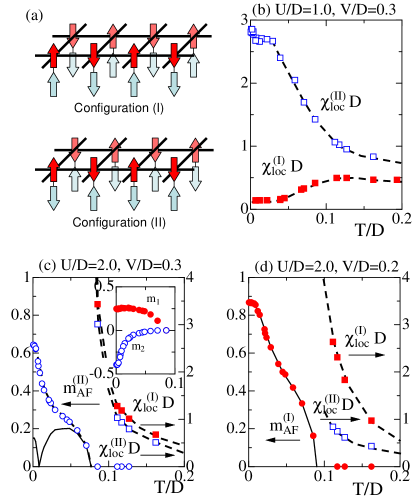
Figure 1: (a) Possible spin configurations. (b), (c) and (d) show the staggered susceptibilities and the magnetizations as a function of the temperature $T$. Solid lines represent $|m_{AF}^{(I)}|$ and dashed lines are guide to eyes. Solid and open symbols represent the results for the configuration (I) and (II).

When $U/D=1.0$ and $V/D=0.3$, no singularity appears in both staggered susceptibilities, as shown in Fig. 1 (b). This suggests that the non-magnetic Kondo singlet ground state is realized at low temperatures. We also find that magnetic fluctuations for the configuration (II) are enhanced at low temperatures and the system is close to the AF (II) state. In fact, when the parameters are slightly changed, the AF (II) state appears at low temperatures. The staggered susceptibility diverges at a critical temperature $T_{N}$ and a spontaneous magnetization $m_{AF}^{(II)}$ appears below $T_{N}$, as shown in Fig. 1 (c). It is also found that a shoulder structure appears in the temperature-dependent magnetization. This implies that magnetic correlations for each band are not enhanced at the same temperature (see also the inset). This interesting feature will be discussed later. On the other hand, when the Coulomb interaction and Hund’s coupling are relatively large ($U/D=2.0$ and $V/D=0.2$), $\chi_{AF}^{(I)}$ diverges at the critical temperature and $m_{AF}^{(I)}$ appears at lower temperatures, as shown in Fig. 1 (d). The AF (I) state is then realized in the ground state.

By performing similar calculations for various model parameters, we end up with the low-temperature phase diagram at half filling, shown in Fig. 2 (a). To discuss the phase transitions between these states in detail, we show in Fig. 2 (b) the staggered magnetization for each band when $V/D=0.3$.

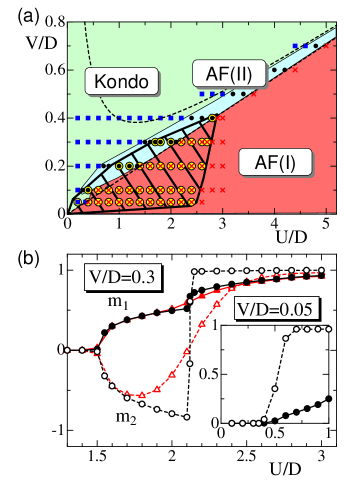
Figure 2: (a) The phase diagram of the EPAM at $T/D=4.6\times 10^{-4}$. Solid squares, crosses and solid circles represent the Kondo singlet, AF (I) and AF (II) phases, respectively. Open circles indicate the metallic state realized in the shaded area, which will be discussed (Fig. 4). The phase boundaries are guide to eyes. Dashed line is the phase boundary obtained from the strong coupling limit. (b) The magnetization for each band when $V/D=0.3$. Circles and triangles represent the results at $T/D=4.6\times 10^{-4}$ and $0.015$, respectively. The inset shows the results for $V/D=0.05$.

In the case of small $U/D$, the interband hybridization screens the local moments, and no magnetizations appear in both bands. Therefore, in the region $(U/D)<(U/D)_{c1}[\sim 1.5]$ the paramagnetic Kondo phase is realized, as shown in Fig. 2 (b). The increase in the interaction induces magnetic moments for both bands with opposite signs. This implies that a continuous phase transition occurs to the AF (II) phase. Further increase in the interaction leads to a jump singularity in the temperature-dependent magnetization, at which the sublattice magnetizations become parallel. The first order phase transition then drives the system to the AF (I) state at $(U/D)_{c2}\sim 2.1$. It is also found that the jump singularity vanishes when the temperature is slightly increased, as shown in Fig. 2 (b). Therefore, the phase transition between two AF states is present at zero temperature only, while a crossover occurs at finite temperatures.

The competition between these phases may be explained by considering the strong coupling limit $(U\rightarrow\infty)$. The system is then reduced to the Kondo necklace Heisenberg model as, $H=J_{inter}\sum_{ij}{\bf S}_{i1}\cdot{\bf S}_{j1}+J_{intra}\sum_{i}{\bf S}_{i1}\cdot{\bf S}_{i2}$, where ${\bf S}_{i\alpha}=\sum_{ss^{\prime}}\frac{1}{2}c_{i\alpha s}^{\dagger}\sigma_{ss^{\prime}}c_{i\alpha s^{\prime}}$, $J_{inter}$ is the intersite effective exchange coupling, and the intrasite one is represented by $J_{intra}$, instead of $J$. We note that $J_{inter}(=4t^{2}/U)$ is always positive, while $J_{intra}$ depends on the interactions and the hybridization. Its magnitude is given by the lowest singlet-triplet gap of the local Hamiltonian $H_{loc}$ as $J_{intra}=\Delta E[=U(\sqrt{\lambda^{2}+4(V/U)^{2}}-3\lambda)]$. In the model, three distinct phases appear in the phase diagram, which is schematically shown in Fig. 3.

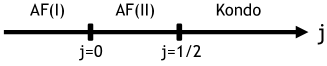
Figure 3: Ground-state phase diagram for the Kondo necklace model.

When $j(=zJ_{intra}/J_{inter})\gg 1$, the Kondo singlet phase is stabilized, where $z$ is the coordination number. An increase in the intersite coupling $J_{inter}$ enhances AF correlations and a second-order phase transition, at last, occurs to the AF (II) phase at a critical value $j_{c}(=1/2)$. The phase boundary obtained from the strong coupling limit, which is given by $(V/D)_{c}=(U/4D)\sqrt{(4\lambda+(D/U)^{2})(8\lambda+(D/U)^{2}}$, is consistent with that in the EPAM, as shown in Fig. 2 (a). On the other hand, the AF (I) and (II) phases are separated by the condition $j=0[V/D=\sqrt{2}\lambda(U/D)]$, where the localized spins ${\bf S}_{i2}$ are completely decoupled and the phase transition never occurs. In contrast, two bands are coupled through the hybridization $V$ in the EPAM, leading to a first-order phase transition. The corresponding phase boundary is in good agreement with the condition $j=0$. When $V/D=0.05$ and $T/D=4.6\times 10^{-4}$, we could not find the AF (II) phase between AF (I) and Kondo insulating phases, as shown in the inset of Fig. 2 (b). This is consistent with the fact that in the weak coupling region the energy scale of magnetic correlations is fairly small and the AF state is stable only at very low temperatures. Therefore, we believe that in the ground-state magnetic phase diagram, the AF (II) phase always appears between the AF (I) and Kondo phases.

Next, we discuss the finite-temperature magnetic properties such as the shoulder structure in the magnetization shown before. When one concentrates on the local Hamiltonian $H_{loc}$, the low-lying singlet and triplet states can be considered to be four-fold degenerate down to a certain temperature $T^{*}=|\Delta E|$. When $T^{*}$ is sufficiently low, an intersite exchange stabilizes the magnetically ordered state, where the itinerant band is almost fully polarized while nearly free localized spins appear in the other. This reveals that orbital-selective like features appear in the intermediate temperature $T^{*}<T<T_{N}$ and magnetic correlations in the localized band are enhanced below $T^{*}$. Such behavior is clearly found in the vicinity of the phase boundary between AF (I) and (II) states, where $T^{*}\ll T_{N}$. In fact, when $U/D=2.0$ and $V/D=0.3$, $(T^{*},T_{N})\sim(0.032D,0.075D)$ and the shoulder structure appears in the temperature-dependent magnetization, as shown in the inset of Fig. 1 (c). Furthermore, we find nontrivial behavior in the observable quantity $|m_{AF}^{(I)}|$. Namely, when decreasing the temperature, it once vanishes at a certain temperature below $T^{*}$, and is induced again, shown as the solid line in Fig. 1 (c). This non-monotonic behavior may be observed in the intensity of the magnetic peak in the inelastic neutron scattering experiments for some transition-metal oxides with localized and itinerant bands such as $\rm Ca_{2-x}Sr_{x}RuO_{4}(0<x<0.5)$, which then allows us to discuss the competition between Hund’s coupling and the hybridization at each site.

We would like to mention another remarkable feature for the metal-insulator (MI) transition at half filling. In infinite dimensions, the Hubbard and the Kondo lattice model have a chance to realize the MI transition without magnetism when the system is strongly frustrated. However, in the system without frustration, the magnetically ordered state is more stable than the paramagnetic metallic state and the Mott insulating state at zero temperature, where the charge gap always opens around the Fermi level. [24, 25] The EPAM treated here is not frustrated, but has competing interactions between the orbitals at each site, which may be referred to as orbital frustration. Therefore, it is not trivial whether the ground state is always insulating under orbital frustration. To clarify this, we show the DOS in Fig. 4 (a).

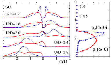
Figure 4: (a) DOS in the system with the majority spin in the itinerant band when $V/D=0.3$ and $U/D=1.2,1.6,2.0,2.4,2.8$ at $T/D=4.6\times 10^{-4}$. (b) DOS at the Fermi level as a function of $U/D$. Solid (dashed) lines represent the results for the itinerant (localized) band.

When $U/D\leq 1.5$, the Kondo insulating state is realized, where the hybridization gap clearly appears in the localized band. In the case $U/D\geq 2.8$, the structures in the DOS in both bands appear far from the Fermi level, where the polarized ground state is realized with the configuration (I). On the other hand, when the system approaches the intermediate region, spectral weight is built up around the Fermi level. In fact, Fig. 4 (b) clearly shows that a finite DOS at each band appears in the intermediate region, although the $\alpha=2$ band is almost localized in the case $(2.4<U<2.8)$. This fact implies that a metallic phase appears between the different insulating states. Since the DOS is continuously changed at the metal-insulator transition points, a drastic change was not found in the magnetization shown in Fig. 2 (b). In our phase diagram, this magnetic metal is stable in the weak coupling region shown as the shaded area in Fig. 2 (a). We recall that when $V=0(U=0)$, the system is reduced to the Kondo lattice (conventional periodic Anderson) model, where the AF (Kondo) insulator is always realized except for the decoupled limit $U=V=0$. Therefore, we claim that the competition between Hund’s coupling and the hybridization introducing a kind of orbital frustration plays an important role in stabilizing the magnetic metal. This is in contrast to the other correlated systems such as the Hubbard model and the Kondo lattice model, where the magnetic insulating state is always realized, as mentioned above.

In summery, we have investigated the extended periodic Anderson model by combining the dynamical mean-field theory with the numerical renormalization group. We have discussed the magnetic properties at low temperatures to clarify how the magnetically ordered states compete with the Kondo insulating state. Furthermore, we have for the first time found the magnetic metallic state in the half-filled system without lattice frustration, which is instead stabilized by orbital frustration.

This work was partly supported by a Grant-in-Aid from the Ministry of Education, Science, Sports and Culture of Japan [19014013 (N.K.), 17740226 (A.K.)] and the German Science Foundation (DFG) through the collaborative research grant SFB 602 (T.P., A.K.) and the project PR 298/10-1 (R.P.) A.K. would in particular like to thank the SFB 602 for its support and hospitality during his stays at the University of Göttingen. Part of the computations were done at the Supercomputer Center at the Institute for Solid State Physics, University of Tokyo and Yukawa Institute Computer Facility.

References

- [1] A. Urushibara, et al., Phys. Rev. B 51, 14103 (1995); Y. Moritomo, et al., Nature 380, 141 (1996).
- [2] S. Nakatsuji, et al., Phys. Rev. Lett. 90, 137202 (2003).
- [3] K. Sreedhar et al., J. Solid State Chem. 110, 208 (1994); Z. Zhang et al., ibid. 108, 402 (1994); 117, 236 (1995).
- [4] Y. Kobayashi, et al., J. Phys. Soc. Jpn. 65, 3978 (1996)
- [5] V. I. Anisimov et al., Eur. Phys. J. B 25, 191 (2002).
- [6] A. Koga, et al., Phys. Rev. Lett. 92, 216402 (2004); Prog. Theor. Phys. Suppl. 160, 253 (2005).
- [7] A. Koga, et al., Phys. Rev. B 72, 045128 (2005).
- [8] L. de’ Medici, et al., Phys. Rev. B 72, 205124 (2005).
- [9] A. Koga, et al., Phys. Rev. B 77, 045120 (2008).
- [10] J. Bünemann, et al., J. Phys. Condens. Matter, 19, 436206 (2007).
- [11] N. Grewe and F. Steglich, in Handbook on the Physics and Chemistry of Rare Earths, edited by K. A. Gschneidner, Jr. and L. Eyring (North-Holland, Amsterdam, 1991), vol. 14, p. 343.
- [12] N. Grewe, Solid State Commun. 50, 19 (1984); K. Yamada, and K. Yoshida, in Theory of Heavy Fermions and Valence Fluctuations, edited by T. Kasuya and T. Saso (Springer, Berlin, 1985); Th. Pruschke, and N. Grewe, Z. Phys. B 74, 439 (1989).
- [13] A.C. Hewson, The Kondo Problem to Heavy Fermions, Cambridge University Press (Cambridge, 1993).
- [14] C. Zener, Phys. Rev. 82, 4031 (1951).
- [15] P. W. Anderson and H. Hasegawa, Phys. Rev. 100, 675 (1955).
- [16] K. Kubo and N. Ohata, J. Phys. Soc. Jpn. 33, 21 (1975).
- [17] N. Furukawa, J. Phys. Soc. Jpn. 64, 2734 (1995).
- [18] W. Metzner and D. Vollhardt, Phys. Rev. Lett. 62, 324 (1989).
- [19] E. Müller-Hartmann, Z. Phys. B 74, 507 (1989).
- [20] A. Georges, et al., Rev. Mod. Phys. 68, 13 (1996).
- [21] T. Pruschke, et al., Adv. Phys. 42, 187 (1995).
- [22] R. Chitra and G. Kotliar, Phys. Rev. Lett. 83, 2386 (1999).
- [23] T. Momoi and K. Kubo, Phys. Rev. B 58, R567 (1998).
- [24] R. Zitzler, et al., Eur. Phys. J. B 27, 473 (2002).
- [25] R. Peters and Th. Pruschke, Phys. Rev. B 76, 245101 (2007).
- [26] T. Schork and S. Blawid, Phys. Rev. B 56, 6559 (1997).
- [27] R. Sato, et al., J. Phys. Soc. Jpn. 73, 1864 (2004).
- [28] H. R. Krishna-murthy, et al., Phys. Rev. B 21, 1003 (1980).
- [29] R. Bulla, et al., cond-mat/0701105 (2007).
- [30] O. Sakai and Y. Kuramoto, Solid State Comm. 89, 307 (1994).
- [31] R. Bulla, Phys. Rev. Lett. 83, 136 (1999).
- [32] F.B. Anders, and A. Schiller, Phys. Rev. B 74, 245113 (2006).
- [33] R. Peters, et al., Phys. Rev. B 74, 245114 (2006).
- [34] A. Weichselbaum and J. von Delft, Phys. Rev. Lett. 99, 076402 (2007).
- [35] T. Ohashi, et al., Phys. Rev. B 70, 245104 (2004).
- [36] I.Milat, et al., Eur. Phys. J. B 38, 571 (2004).