Determination of target thickness and luminosity from beam energy losses

Abstract

The repeated passage of a coasting ion beam of a storage ring through a thin target induces a shift in the revolution frequency due to the energy loss in the target. Since the frequency shift is proportional to the beam-target overlap, its measurement offers the possibility of determining the target thickness and hence the corresponding luminosity in an experiment. This effect has been investigated with an internal proton beam of energy 2.65 GeV at the COSY-Jülich accelerator using the ANKE spectrometer and a hydrogen cluster-jet target. Possible sources of error, especially those arising from the influence of residual gas in the ring, were carefully studied, resulting in a accuracy of better than 5%. The luminosity determined in this way was used, in conjunction with measurements in the ANKE forward detector, to determine the cross section for elastic proton-proton scattering. The result is compared to published data as well as to the predictions of a phase shift solution. The practicability and the limitations of the energy-loss method are discussed.

I Introduction

In an ideal scattering experiment with an external beam, the particles pass through a wide homogeneous target of known thickness. If the fluxes of the incident and scattered particles are measured, the absolute cross section of a reaction can be determined. The situation is far more complicated for experiments with an internal target at a storage ring where the target thickness cannot be simply established through macroscopic measurements. In such a case the overall normalization of the cross section is not fixed though one can, for example, study an angular dependence or measure the ratio of two cross sections. If the value of one of these cross sections is known by independent means, the ratio would allow the other to be determined. However, there are often difficulties in finding a suitable calibration reaction and so it is highly desirable to find an alternative way to measure the effective target thickness inside a storage ring.

When a charged particle passes through matter it loses energy through electromagnetic processes and this is also true inside a storage ring where a coasting beam goes through a thin target a very large number of times. The energy loss, which is proportional to the target thickness, builds up steadily in time and causes a shift in the frequency of revolution in the machine which can be measured through the study of the Schottky spectra Zapfe . Knowing the characteristics of the machine and, assuming that other contributions to the energy loss outside the target are negligible or can be corrected for, this allows the effective target thickness to be deduced. It is the purpose of this article to show how this procedure could be implemented at the COSY storage ring of the Forschungszentrum Jülich.

The count rate $n$ of a detector system which selects a specific reaction is given by

$$n=L\left(\frac{d\sigma}{d\Omega}\right)\Delta\Omega\,,$$ (1)

where $d\sigma/d\Omega$ is the cross section, $\Delta\Omega$ the solid angle of the detector and $L$ the beam-target luminosity. This is related to the effective target thickness $n_{T}$, expressed as an areal density, through

$$L=n_{B}\,n_{T}\,,$$ (2)

where $n_{B}$ is the particle current of the incident beam.

Figure 1: Top view of the ANKE spectrometer and detectors Bar01 ; Har07 . The spectrometer contains three dipole magnets D1, D2, and D3, which guide the circulating COSY beam through a chicane. The central C-shaped spectrometer dipole D2, placed downstream of the target, separates the reaction products from the beam. The ANKE detection system, comprising range telescopes, scintillation counters and multi-wire proportional chambers, registers simultaneously negatively and positively charged particles and measures their momenta. The silicon tracking telescopes (STT) placed in the target chamber are used to measure low energy recoils from the target.

The luminosity, rather than the target thickness, is the primary quantity that has to be known in order to evaluate a cross section through Eq. (1). The measurement of a calibration reaction, such as proton-proton elastic scattering, leads directly to a determination of the luminosity. In contrast, the energy-loss technique described here yields directly an estimate of the effective target thickness, but this can be converted into one of luminosity through the measurement of the beam current, which can be done to high accuracy using a beam current transformer.

Originally, the frequency-shift measurements were carried out and analyzed at ANKE using only a few accelerator cycles over the extended run of a specific experiment in order to get a rough estimate of the available luminosity. However, a careful audit of the various error sources has now been conducted to find out the accuracy that can be achieved. Energy-loss measurements are therefore now routinely carried out in conjunction with the experimental data-taking.

A brief presentation of the overall layout of the ANKE spectrometer in the COSY ring is to be found in Sec. II with the operation of COSY for this investigation being described in Sec. III. The basic theory and formulae that relate the target thickness to the change in revolution frequency are presented in Sec. IV, where the modifications caused by the growth in the beam emittance are also explained. The application of the energy-loss method to the measurement of the target thickness for typical target conditions when using a proton beam with an energy of 2.65 GeV is the object of Sec. V. A careful consideration is given here to the different possible sources of error. These errors are also the dominant ones for the luminosity discussed in Sec. VI. It is shown there that the relative luminosity is already well determined through the use of monitor counters so that the absolute luminosity given by the energy-loss measurement needs only to be investigated for a sub-sample of typical cycles. A comparison is made with the luminosity measured through elastic proton-proton scattering at 2.65 GeV, though this is hampered by the limited data base existing at small angles. Our summary and outlook for the future of the energy-loss technique are offered in Sec. VII.

II COSY and the ANKE spectrometer

COSY is a COoler SYnchrotron that is capable of accelerating and storing protons or deuterons, polarized and unpolarized, for momenta up to 3.7 GeV/$c$, corresponding to an energy of 2.9 GeV for protons and 2.3 GeV for deuterons Mai97 .

The ANKE magnetic spectrometer Bar01 ; Har07 , which is located inside one of the straight sections of the racetrack-shaped 183 m long COSY ring, is a facility designed for the study of a wide variety of hadronic reactions. The accelerator beam hits the target placed in front of the main spectrometer magnet D2, as shown in Fig. 1. An assembly of various detectors indicated in the figure allows, in combination with the data-processing electronics, for the identification and measurement of many diverse reactions. The method of determining the luminosity from the beam energy loss in the target should be applicable to the cases of the hydrogen and deuterium gas in cluster-jet targets or storage cells that are routinely used at ANKE. However, due to the short lifetime of the beam, the technique is unlikely to be viable for the foil targets that are sometimes used for nuclear studies.

III Machine Operation

We discuss in detail the operational conditions of the 2004 beam time where $\phi$-meson production in the $pp\to{}pp\phi$ reaction was studied Har06 . The proton beam with an energy of 2.650 GeV was incident on a hydrogen cluster-jet target with a diameter of 7 mm Mue04 . In order to accelerate the proton beam from the injection energy of $T=45$ MeV, a special procedure is used at COSY which avoids the crossing of the critical transition energy $T_{\text{tr}}=mc^{2}(\gamma_{\text{tr}}-1)$ Mai97 . For this purpose, a lattice setting that has a transition energy of about 1 GeV is used at injection. During the acceleration the ion optics in the arcs is manipulated such that the transition energy is dynamically shifted upward. After the requested energy is reached, the acceleration (rf) cavity is switched off and the ion optics manipulated again such that the dispersion $D$ in both straight sections vanishes. The transition energy is then about 2.3 GeV, i.e. the experiment used a coasting beam above the transition. Furthermore, the optics is slightly adjusted to place the working point $(Q_{x},Q_{y})$ in the resonance-free region of the machine between 3.60 and 3.66. This guarantees that beam losses due machine resonances are avoided. The resulting optical functions $\beta_{x}$, $\beta_{y}$, and dispersion $D$ of the COSY ring, calculated within a linear optics model, are shown in Fig. 2.

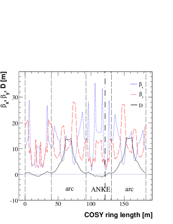
Figure 2: (Color online) Ion optical functions around the COSY ring as adjusted for experiments at ANKE. Here $\beta_{x}$ (dotted line), $\beta_{y}$ (dashed line) are the horizontal and vertical beta functions and $D$ (solid line) is the dispersion.

At the ANKE target position the parameters are $\beta_{x}=2.4$ m and $\beta_{y}=3.0$ m. Orbit measurements have validated that the dispersion is here within the range $\pm\,0.5$ m. Since $D\approx 0$ in this region, the ion beam does not move away from the target when its energy decreases. The ion beam losses occur dominantly in the arcs, where the machine acceptance is lower due to the large dispersion of up to 15 m. Experience has shown that, depending upon the actual target thickness, experiments with the cluster-jet target can be run with cycle times of 5-10 minutes with little ion beam losses.

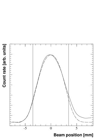
Figure 3: Transverse beam-target overlap profile. The solid curve shows the measured profile while the dashed line shows the predicted one. The vertical lines represent the measured diameter of the cluster-jet beam.

The maximum of the beam-target interaction was found by steering horizontally the proton beam continuously through the target and identifying the highest count rate in the forward detector system which was used as a monitor. The measured overlap profile shown in Fig. 3 also contains information about the proton beam size. The predicted profile was obtained by convoluting a cylindrical cluster-jet beam of uniform density and 7 mm diameter Mue04 with a Gaussian proton beam profile of width $\sigma_{x}=1.2$ mm. Despite the idealized assumptions, the measured profile is reasonably well reproduced. The maximum overlap varies by less than 10% for $\sigma_{x}$ in the range from 1.0 to 1.5 mm.

The proton beam profile was independently investigated by scraping the beam at the target position with a diaphragm oriented perpendicular to the beam, which was moved through the beam. This yielded a Gaussian beam profile with a total width $4\sigma\approx 5\,$mm Leh04 . Later dedicated measurements have also confirmed the typical size of the beam Kirill .

The beam-target interaction, i.e. the effective target thickness, might decrease during a machine cycle. This could arise from emittance growth or the dispersion not being exactly zero and would induce a slight nonlinear time dependence of the frequency shift. Emittance growth and effective target thickness are discussed in Secs. IV.2 and V.

IV Beam-target interaction, energy loss and emittance growth

The fact that most ANKE experiments ran with a coasting beam without cooling offered the possibility for using the energy loss in the target as a direct and independent method for luminosity calibration.

IV.1 Energy loss

The energy loss $\delta T$ per single target traversal, divided by the stopping power $dE/dx$ and the mass $m$ of the target atom, yields the number $n_{T}$ of target atoms per unit area that interact with the ion beam:

$$n_{T}=\frac{\delta T}{(dE/dx)m}\,\cdot$$ (3)

Over a small time interval $\Delta t$, the beam makes $f_{0}\Delta t$ traversals, where $f_{0}$ is the revolution frequency of the machine. If the corresponding energy loss is $\Delta T$, Eq. (3) may be rewritten as:

$$n_{T}=\frac{\Delta T}{f_{0}(dE/dx)m\,\Delta t}$$ (4)

or, in terms of the change in the beam momentum $p$, as

$$n_{T}=\left(\frac{1+\gamma}{\gamma}\right)\frac{T_{0}\Delta p}{f_{0}(dE/dx)mp_{0}\Delta t}\,,$$ (5)

where $T_{0}$ and $p_{0}$ are the initial values of the beam energy and momentum, and $\gamma=(1-\beta^{2})^{-1/2}$ is the Lorentz factor.

In a closed orbit, the fractional change in the revolution frequency is proportional to that in the momentum:

$$\frac{\Delta p}{p_{0}}=\frac{1}{\eta}\frac{\Delta f}{f_{0}}\,,$$ (6)

where $\eta$ is the so-called frequency-slip parameter.

Putting these expressions together, we obtain

$$n_{T}=\left(\frac{1+\gamma}{\gamma}\right)\frac{1}{\eta}\frac{1}{(dE/dx)m}\,\frac{T_{0}}{f_{0}^{2}}\,\frac{df}{dt}\,\cdot$$ (7)

In order to be able to deduce absolute values for the target thickness on the basis of Eq. (7), it is necessary to determine $\eta$ with good accuracy. The revolution frequency depends on the particle speed $\beta c$ and orbit length $C$ through $f=\beta c/C$ where, due to dispersion, $C$ is also a function of the momentum. Defining $dC/C=\alpha\,dp/p$, we see that

$$\frac{df}{f}=\left(\frac{1}{\gamma^{2}}-\alpha\right)\frac{dp}{p}\,\cdot$$ (8)

Here $\alpha$ is the so-called momentum compaction factor, which is a constant for a given lattice setting. The point of transition, where $df$ changes its sign, occurs when $\alpha=1/\gamma^{2}$. Generally, $\alpha$ lies between 0 and 1, so that $df$ is negative below and positive above transition. In terms of $\alpha=1/\gamma_{\text{tr}}^{2}$, the expression for $\eta$ reads:

$$\eta=\frac{1}{\gamma^{2}}-\frac{1}{\gamma_{\text{tr}}^{2}}\,\cdot$$ (9)

The value of $\gamma$ is fixed by the beam momentum, which is known with an accuracy on the order of 10^-3. The value of $\gamma_{\text{tr}}$ is fixed for an individual setting of the accelerator lattice used in the experiment. Near the transition point $\eta$ is small and this is the principal restriction on the applicability of the frequency-shift method.

An estimate for $\gamma_{\text{tr}}$ may be made using lattice models but, to obtain more reliable values, a measurement of $\alpha$ is indispensable. This is done by changing the magnetic field $B$ in the bending magnets by a few parts per thousand and using

$$\frac{\Delta f}{f}=\alpha\,\frac{\Delta B}{B}\,\cdot$$ (10)

IV.2 Emittance growth

In addition to energy loss, the beam also experiences emittance growth through the multiple small angle Coulomb scattering in the target. At each target traversal the emittance of the ion beam increases slightly in both directions and, as a consequence, the beam-target overlap may be reduced. As discussed in Sec. III, both $D$ and $D^{\prime}$ are practically zero in the ANKE region. In this case, the rate of emittance $\epsilon$ growth is given by Hin89 :

$$\frac{d\epsilon}{dt}=\mbox{${\textstyle\frac{1}{2}}$}f_{0}\beta_{T}\theta_{\text{rms}}^{2}\>,$$ (11)

where $\beta_{T}$ represents the value of the beta function at the position of the target, and $\theta_{\text{rms}}$ the projected rms scattering angle for a single target traversal. The $1/2$ factor comes from integrating over the phases of the particle motion in the ion beam.

The value of $\theta_{\text{rms}}$ can be estimated from

$$\theta_{\text{rms}}=Z\frac{14.1\,\textrm{MeV}}{\beta cp}\sqrt{\frac{x}{X_{0}}}\>,$$ (12)

where $Z$ is the charge number of the incident particle and $x/X_{0}$ the target thickness in units of the radiation length $X_{0}$ Hin89 .

The final rms beam width $w_{f}$ after an emittance growth $\Delta\epsilon$ is given by

$$w_{f}=\sqrt{w_{i}^{2}+\beta_{T}\,\Delta\epsilon}\>.$$ (13)

Under typical experimental conditions of a proton beam incident on a cluster-jet target containing $n_{T}=2\times 10^{14}\textrm{cm}^{-2}$ hydrogen atoms, an initial horizontal width of $w_{x,i}=1.2$ mm increases to only 1.36 mm over a 10 min period. This suggests that the beam-target overlap or effective target thickness should be constant to within 5% and that the frequency shift should show a linear time dependence.

V Measurement of target thickness by energy loss

Table 1: Parameters relevant for the target thickness evaluation at 2.650 GeV

Parameters	Values
$f_{0}=$ initial revolution frequency	1.57695 MHz
$\beta=v/c=$ particle speed based on $f_{0}$ and $C_{\text{nom}}=183.493$ m (including ANKE chicane)	0.9652
$\gamma=(1-\beta^{2})^{-1/2}=$ Lorentz factor	3.824
$p_{0}=\beta\gamma mc=$ beam momentum	3.463 GeV/c
$T_{0}=(\gamma-1)mc^{2}=$ beam kinetic energy	2.650 GeV
$\alpha=$ momentum compaction factor	$0.183\pm 0.003$
$\eta=$ frequency-slip parameter evaluated from the measured value of $\alpha$	$-0.115\pm 0.003$
$dE/dx=$ stopping power of protons in hydrogen gas	$4.108\,$MeV cm2 g-1 NIS

The parameters required for the estimation of the target thickness for the experiment under consideration are given in Table 1. Here $\beta$, $\gamma$, $p_{0}$, and $T_{0}$ are determined by the measured revolution frequency and nominal circumference of the accelerator and $dE/dx$ is evaluated from the Bethe-Bloch formula as is done, e.g., in Ref. NIS . The frequency shift $\Delta f$ is measured by analyzing the Schottky noise of the coasting proton beam and the momentum compaction factor $\alpha$, and hence the $\eta$-parameter, by studying the effects of making small changes in the magnetic field.

The origin of the Schottky noise is the statistical distribution of the particles in the beam. This gives rise to current fluctuations which induce a voltage signal at a beam pick-up. The Fourier analysis of the voltage signal, i.e. of the random current fluctuations, by a spectrum analyzer delivers frequency distributions around the harmonics of the revolution frequency. For this purpose we used the pick-up and the spectrum analyzer (standard swept-type model HP 8753D) of the stochastic cooling system of COSY Sto , which was operated at harmonic number 1000. During the experimental runs with a target, the Schottky spectra around 1.577 GHz were measured every minute over the 566 s long cycle, thus giving ten sets of data per cycle. The frequency span was 600 kHz and the resolution 1 kHz. The sweep time of the analyzer was set to 6 s so that, to a good approximation, instantaneous spectra were measured, which were then directly transferred to the central data acquisition of ANKE for later evaluation.

The spectrum analyzer measures primarily the Schottky noise current, which is proportional to the square root of the number $N$ of particles in the ring. The amplitudes of the measured distributions are therefore squared to give the Schottky power spectra, which are representative of the momentum distribution Bou87 . The centroids of these power spectra yield the frequency shifts needed for the calculation of the mean energy losses. It must be emphasized here that, by definition, the Bethe-Bloch $dE/dx$ refers to the mean energy loss.

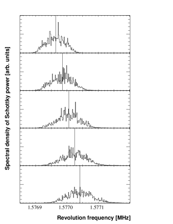
Figure 4: Schottky power spectra obtained during one ten-minute cycle and scaled to harmonic number 1. Although the data were recorded every minute, for ease of presentation, only the results from the even minutes are shown, starting from top to bottom. Each spectrum is a true representation of the momentum distribution, and the shift over the cycle is a measure for the energy loss. The mean frequencies resulting from the fits are indicated by the vertical lines. Since these data were taken above the transition energy, $\eta$ is negative and the frequency increases through the cycle.

Figure 4 shows a typical result for the Schottky power spectra obtained during one of the ten minute cycles. Due to the momentum spread of the coasting beam, the spectra have finite widths. The overall frequency shift in the cycle, which is comparable to the width, is positive because at 2.65 GeV the accelerator is working above the transition point. Even the final spectrum in Fig. 4 fits well into the longitudinal acceptance and there is no sign of any cut on the high frequency side. The background was estimated by excluding data within $\pm 3\sigma$ of the peak position. After subtracting this from the original spectrum, the mean values of the frequency distribution was evaluated numerically.

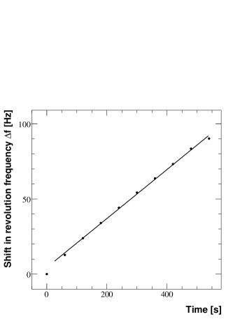
Figure 5: Typical mean frequency shifts derived from the Schottky power spectra of the type illustrated in Fig. 4 at ten equally spaced intervals of time. These results show a linear increase with time with a slope $df/dt=(0.163\pm 0.003)\,$Hz/s. The first point was omitted from this fit since it was taken too early in the cycle when the COSY magnets have not reached their steady state after the acceleration.

The time dependence of the mean revolution frequency shift $\Delta f$ is shown for a typical cycle in Fig. 5. It is well described by a linear function, which is consistent with the assumption that the beam-target overlap changes little over the cycle. This means that the emittance growth is negligible and that there is no significant shift of the proton beam arising from a possible residual dispersion. A linear fit over the particular cycle considered here gives a slope of $df/dt=(0.163\pm 0.003)$ Hz/s.

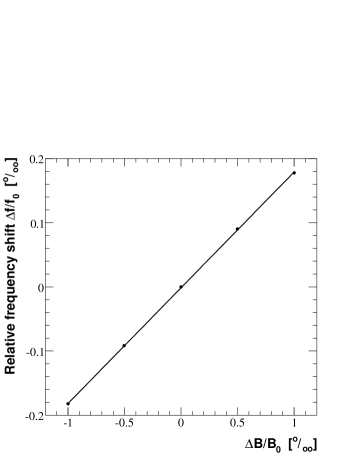
Figure 6: Variation of the mean revolution frequency with the field strength in the bending magnets in parts per thousand. The slope of the fitted straight line yields the value of the momentum compaction factor $\alpha$.

The value of the frequency-slip parameter $\eta$ was obtained by measuring the momentum compaction factor $\alpha$ using separate machine cycles without target. The shift of the mean revolution frequency as a function of the $\Delta B/B_{0}$ change in the bending magnets was investigated in the same way as for the energy loss by determining the mean value of the frequency distributions. Figure 6 shows the five measured points for the relative frequency shift $\Delta f/f_{0}$ as a function of $\Delta B/B_{0}$ in the range from $-1.0$ to $+1.0$ per mille, in steps of 0.5 per mille. The straight line fit, which is a good representation of the data, leads to a value of the slope. These measurements were carried out on three separate occasions during the course of the four-week run and consistent values of the slope were obtained, from which we deduced that $\alpha=0.183\pm 0.003$, and hence $\eta=-0.115\pm 0.003$.

Using Eq. (7), a first approximation to the value of the effective target thickness can now be given, assuming that the measured frequency shift is dominantly caused by the target itself. The result for the particular machine cycle, which is typical for the whole run, is $n_{T}=2.8\times 10^{14}$ cm^-2. This result contains, of course, a contribution arising from the residual gas in the ring. The systematic correction that is needed to take account of this is discussed in the following section.

V.1 Systematic correction for residual gas effects

The contribution of the residual gas in the ring to the energy loss was measured in some cycles with the target switched off. The resulting frequency shift rate was $df/dt=(0.008\pm 0.003)$ Hz/s, which corresponds to a 5% effect as compared to that obtained with the target. The measurement was repeated a few times during the four weeks of the experiment and the result was reproducible to within errors. This is consistent with the observation that the pressure in the ring was stable.

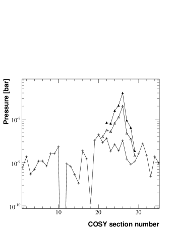
Figure 7: Vacuum pressure profile along sections of the COSY ring; ANKE is placed close to section number 26. Crosses show the pressure profile for the situation when the (cluster-jet) target beam is off, the increase illustrated by the open triangles is due to the target-on effect, and the closed triangles that when the COSY beam is allowed to interact with the target jet. The lines are drawn to guide the eye.

However, as seen from Fig. 7, the gas pressure rises in the vicinity of ANKE when the target is switched on. The figure shows the vacuum pressure profile along the 183 m long ring for the three conditions (a) target off and no proton beam, (b) target on and no proton beam, (c) target on and proton beam incident on the target. A pressure bump with a maximum in the target chamber region is spread over a region of about $\pm 5$ m, up- and downstream of the target position, which is in the vicinity of section 26. The pressure in the target vacuum chamber was $4\times 10^{-9}$ mbar with the target off, which is about twice the average over the whole ring. With the target on this pressure reached $2\times 10^{-8}$ mbar and further increased to $4\times 10^{-8}$ mbar when the proton beam interacted fully with the target. The pressure rise is obviously caused by hydrogen gas not being completely trapped in the gas catcher. The additional pressure increase when the proton beam hits the target might be attributed to hydrogen gas originating from the cluster-jet target or from the chamber walls after hits by protons in the beam.

One critical question is how much of the energy loss is caused by hydrogen atoms that are not localized in the target beam. This effect was examined by steering the proton beam to positions to the right and left of the target beam. The result was encouraging since $df/dt$ increased only a little to a value of $(0.010\pm 0.002)$ Hz/s. We therefore take $df/dt=(0.012\pm 0.004)$ Hz/s when the proton beam hits the target and the pressure is doubled. As a cross check, the areal density of hydrogen atoms in a 10 m long path of hydrogen gas at the measured pressure of $4\times 10^{-8}$ mbar was calculated and compared to the areal density found for the target. After making corrections for using the pressure gauge with hydrogen rather than air, the areal density of hydrogen atoms was found to be $4.8\times 10^{12}$ cm^-2. Compared to the $n_{T}=2.7\times 10^{14}$ cm^-2 initially estimated, this is only a 2% effect, which confirms the result found from the frequency shift measurement.

It can be assumed that the contribution of hydrogen to the residual gas is proportional to the target thickness. Nevertheless, the uncertainty is large and the final modification of $df/dt$ reads:

$$(df/dt)_{\text{corr}}=\zeta\left[(df/dt)_{\text{total}}-(df/dt)_{\text{ring}}\right]\,,$$ (14)

with $\zeta=0.97\pm 0.02$.

V.2 Uncertainties in the target thickness determination

It is obvious from Eq. (7) that the only significant uncertainty in the determination of the overall target thickness arises from the measurement of the frequency shift $\Delta f$. This error is primarily instrumental in nature. The fit gives an uncertainty of $\pm 2\%$ for the total frequency shift. The systematic correction due to the residual hydrogen gas amounts to $\pm 2\%$. Depending on the variation of the target density during the whole experiment, the relative error in the correction for the ring vacuum was between 1.5 and 3% and the machine parameter $\eta$ contributes a further $\pm 3\%$. These uncertainties, which are summarized in Table 2, stem from independent measurements so that they can be added quadratically to give a total of about 5%. For the cycle under study, the corrected value of the effective target thickness then becomes

$$n_{T}=(2.6\pm 0.13)\times 10^{14}\textrm{cm}^{2}\,.$$

Table 2: Individual contributions to the uncertainty in the determination of the effective target thickness from the beam energy losses. The total uncertainty has been obtained by adding the individual elements quadratically.

Uncertainty	[%]
Frequency shift $\Delta f(t)$	2
Residual gas (ring)	(1.5 - 3)
Residual gas (target section)	2
Frequency-slip parameter ($\eta$)	3
Total	5

It should be noted that the ring gas effect in the present case was only 5% of that due to the target. If the target were much thinner, the uncertainty arising from the residual gas would dominate the total error.

VI Luminosity deduced from the effective target thickness

As seen from Eq. (2), the luminosity can be deduced from the effective target thickness by multiplying by the mean ion particle current $n_{B}$ as determined in the same cycle.

VI.1 Particle current measurement

The beam current $i_{B}=n_{B}e$ was measured by means of a high precision beam current transformer (BCT) which was calibrated to deliver a voltage signal of 100 mV for a 1 mA current. The BCT signal was continuously recorded by the ANKE data acquisition system via an ADC. The accuracy of the BCT is specified to be $10^{-4}$, though care has to be taken to avoid effects from stray magnetic fields. The BCT was therefore mounted in a field-free region of the ring and, in addition, was magnetically shielded. It was calibrated with a current-carrying wire placed between the beam tube and ferrite core of the BCT. Applying a current from a high precision source in the range from $-10$ to $+10$ mA, the linearity and offset of the signal recorded in the data acquisition system were $3\times 10^{-4}$ and 0.2 mV (corresponding to 0.002 mA), respectively. In comparison to the uncertainty of the target thickness, the error in the measurement of proton particle current is negligible since the beam current was typically 10 mA.

VI.2 Luminosity determination

Figure 8(a) shows the proton particle current $n_{B}$ for successive cycles. Within each cycle the current decreases slightly with time due to beam losses from the diminishing acceptance during the cycle which arise from the large dispersion in the arcs. Since the initial beam current also varies a little from cycle to cycle, the mean value $<n_{B}>$, and hence the luminosity, has to be determined for each cycle. This yields the mean or integrated luminosity over a certain period of time which can then be compared directly with the results derived from $pp$ elastic scattering or other calibration reaction.

Figure 8(b) illustrates the count rate $n_{M}$ of a monitor for relative luminosity. For this purpose, the sum signal of the start counters along the analyzing magnet D2 of Fig. 1 has been selected. These counts originate mainly from beam-target interactions, though there is some background that does not come directly from the target. Nevertheless, it is plausible to consider that the background rate is also proportional to the proton beam intensity and target density. That this is largely true is borne out by Fig. 8(c), where the ratio of $n_{M}/n_{B}$ is plotted. Except for a slight increase at the end of each cycle, the ratio is constant within a cycle. This demonstrates that the effective target thickness is constant, as already indicated by the linear time dependence of the frequency shift. This behavior was found to be true for all cycles in the experiment so that the monitor count rate could be used as a good relative measure of the luminosity over the whole experiment run. As a consequence, it is sufficient to calibrate the monitor count rate by determining the effective target density and mean ion particle current for only a few representative cycles.

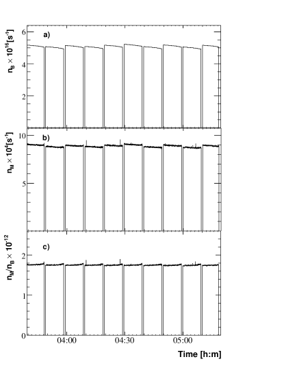
Figure 8: (a) The BCT particle current $n_{B}$, (b) The monitor rate $n_{M}$, and (c) The ratio $n_{M}/n_{B}$, for a sample of machine cycles.

Since the measurement of the beam current with the BCT is accurate to 0.1%, the total uncertainty in the determination of the luminosity via the beam energy-loss method is 5%, the same as for the target thickness shown in Table 2. The values of the luminosity obtained during the experiment ranged between 1.3 and $2.7\times 10^{31}\,\textrm{cm}^{-2}\textrm{s}^{-1}$.

VI.3 Comparison with proton-proton elastic scattering

As an independent check on the energy-loss method, we have measured the small angle elastic proton-proton differential cross section. For this purpose the momentum of a forward-going proton was determined using the ANKE forward detector, which covers laboratory angles between about $4.5^{\circ}$ and $9.0^{\circ}$. The large $pp$ elastic cross section, combined with the momentum resolution of the forward detector, allows one to distinguish easily elastically scattered protons from other events, as seen from the missing-mass distribution shown in Fig. 9.

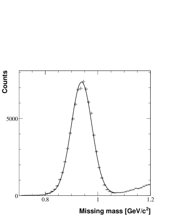
Figure 9: Spectrum of missing masses measured for the $pp\to pX$ reaction at 2.65 GeV showing a proton peak compared to a Gaussian fit. This peak can be cleanly separated from the contributions from pion production which start at 1.07 GeV/$c^{2}$.

After making small background subtractions, as well as correcting for efficiencies and acceptances, the number of detected $pp$ elastic scattering counts per solid angle, $dN_{pp}/d\Omega$, was extracted as a function of the laboratory scattering angle. These were converted into cross sections through Eq. (1) using the values of the luminosities deduced for each run using the energy-loss technique. The individual contributions to the systematic uncertainties in the cross sections are given in Table 3. If these are added quadratically, the overall error is $\pm 12\%$, which is twice as large as the error in the luminosity determined by the beam-energy loss method.

Table 3: Systematic uncertainties in the measurement of the cross section for $pp$ elastic scattering at $T_{p}=2.65$ GeV. The total error has been obtained by adding the individual elements quadratically.

Uncertainty	[$\%$]
Track reconstruction efficiency	5
Acceptance correction	8
Momentum reconstruction	1
Data-taking efficiency	5
Background subtraction	3
Luminosity	5
Total	12

The values found for the proton-proton elastic differential cross section at 2.65 GeV are shown in Fig. 10 together with the current (SP07) solution obtained from the SAID analysis group SAID ; SAID-update . In general the SAID program does not provide error predictions, but these have been estimated by R.A. Arndt Arndt to be on the few percent level for our conditions.

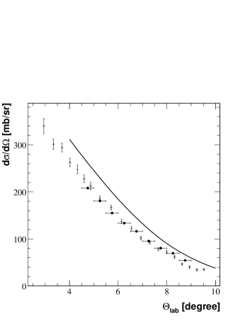
Figure 10: Laboratory differential cross section for elastic proton-proton scattering at 2.65 GeV. Our points, shown by closed circles with bin widths, have systematic uncertainties of $\pm 12$%, as shown in Table 3. The curve is the SP07 solution from the SAID analysis group SAID ; SAID-update and the crosses are experimental data at 2.83 GeV Amb74 .

The shape of the SAID curve is quite similar to that of our data but these points lie about 20% below the predictions SAID ; SAID-update . Such a discrepancy is larger than the overall systematic uncertainty detailed in Table 3. It should also be stressed that the SP07 SAID solution also significantly overestimates the small angle data of both Ambats et al. Amb74 at 2.83 GeV (shown in Fig. 10) and Fujii et al. Fuj62 at 2.87 GeV. It is therefore reassuring to note the disclaimer in the recent SAID update, which states that ‘our solution should be considered at best qualitative between 2.5 and 3 GeV’ SAID-update . This demonstrates clearly the need for more good data in this region.

VII Summary and outlook

We have shown that, under the specific experimental conditions described here, the energy loss of a freely circulating (coasting) ion beam interacting with a cluster-jet target can be used to determine target thickness and beam-target luminosity. The method is simple in principle and independent of the properties of particle detectors which are involved in other techniques such as, e.g., the comparison with elastic scattering. It relies on the fact that the particles in a circulating beam pass through the target more or less the same number of times so that they build up the same energy shift. This is broadly true for the experiment reported here, as can be seen from the fact that the Schottky spectrum at the end of the cycle shown in Fig. 4 has a similar shape to that at the beginning.

Relative measurements of the luminosity are straightforward and quick to perform during a run. The example given here involved the ratio of a monitor rate $n_{M}$ and proton beam current $i_{B}$. Such essentially instantaneous measurements have the advantage that defective cycles with, e.g., a malfunction of the target, the ion beam, or the detection system, can easily be removed from the data analysis. The calibration of such relative measurements through the energy-loss determination needs only to be done from time to time and not for all runs.

The 5% precision reported here for proton-proton collisions at 2.65 GeV is mainly defined by the accuracy of the measured frequency shifts. If the $pp$ elastic differential cross section were known to say 5%, it is seen from Table 3 that the luminosity would only be evaluated using this information at ANKE to about 12%, which is much inferior to the energy-loss method. However, the situation can be quite different at other energies or for other targets.

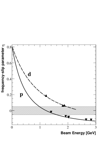
Figure 11: Frequency-slip parameter $\eta$ as a function of the energy of proton and deuteron beams. The experimental points are the results of ANKE measurements during diverse beam runs. These are compared with curves corresponding to the predictions of COSY lattice calculations. The shaded area shows the region with $|\eta|<0.05$ where the error in the energy-loss technique can be high.

The relative error in the frequency-slip parameter $\eta$ of Eq. (9) becomes very large when $\gamma$ is in the region of $\gamma_{\text{tr}}$. For the lattice setting normally applied in ANKE experiments, where $\gamma_{\text{tr}}\approx 2.3$ and the corresponding proton transition energy $T_{\text{tr}}\approx 1.2$ GeV, the beam energy range from 1.0 to 1.6 GeV is not well suited for the energy-loss technique.

The application of the energy-loss technique to deuteron beams and/or deuterium cluster-jet targets goes through identically. For deuteron beams the method can be used over almost the whole of the COSY energy range. This is illustrated clearly in Fig. 11, which shows various measurements of the $\eta$ parameter for both proton and deuteron beams compared with estimates from COSY lattice calculations. The shaded area represents the region of small $\eta$ where the method is of limited use.

The energy-loss method could be particularly valuable for deuterons since, in such cases, there is often a lack of reliable $pd$ elastic or quasi-elastic data Mae06 . Furthermore, when using small angle elastic $dp$ cross sections for normalization, it has to be recognized that this varies exceedingly fast with momentum transfer. As a consequence, even a small error in the determination of the angle must be avoided or otherwise the calibration can be seriously undermined Timo2007 . Since the energy loss is of electromagnetic origin, it could equally well be used with beams of $\alpha$-particles or heavier ions.

The density of a cluster-jet target may be the ideal compromise for implementing the energy-loss approach to luminosity studies. Very thin foils are sometimes used as targets at ANKE Koptev and the beam then dies too quickly for reliable frequency shifts to be extracted. On the other hand, targets of polarized gas in storage cells are very important for the future physics program at ANKE SPIN . The overall target thickness is less than that with the cluster jet so that the ring-gas will provide a larger fraction of the energy loss. The ring-gas effects will also be more important because of greater contamination of the vacuum by the target. It is therefore clear that a detailed analysis of the specific conditions is required to determine the accuracy to be expected in a particular experiment.

References

- (1) K. Zapfe et al., Nucl. Instrum. Methods Phys. Res. A 368, 293 (1996).
- (2) R. Maier et al., Nucl. Instrum. Methods Phys. Res. A 390, 1 (1997).
- (3) S. Barsov et al., Nucl. Instrum. Methods Phys. Res. A 462, 354 (2001).
- (4) M. Hartmann et al., Int. J. Mod. Phys. A 22, 317 (2007).
- (5) M. Hartmann et al., Phys. Rev. Lett. 96, 242301 (2006).
- (6) A. Khoukaz et al., Eur. Phys. J. D 5, 275 (1999); personal communication (2004).
- (7) I. Lehmann, personal communication (2004).
- (8) K. Grigoryev et al., (in preparation).
- (9) F. Hinterberger and D. Prasuhn, Nucl. Instrum. Methods Phys. Res. A 279, 413 (1989).
- (10) M. J. Berger, J. S. Coursey, M. A. Zucker and J. Chang, NIST tables, http://www.physics.nist.gov/PhysRefData/Star/Text/contents.html.
- (11) W.-M. Yao et al., J. Phys. G 33, 1 (2006).
- (12) D. Prasuhn et al., Nucl. Instrum. Methods Phys. Res. A 441, 167 (2000).
- (13) D. Boussard, in Proceedings of CERN Accelerator School: Advanced Accelerator Physics, edited by S. Turner (CERN 87-03, 1987), p. 416.
- (14) R. A. Arndt, I. I. Strakovsky, and R. L. Workman, Phys. Rev. C 62, 034005 (2000); http://gwdac.phys.gwu.edu/.
- (15) R. A. Arndt, W. J. Briscoe, I. I. Strakovsky, and R. L. Workman, Phys. Rev. C 76, 025209 (2007); arXiv:0706.2195v3 [nucl-th] (2007).
- (16) I. Ambats et al., Phys. Rev. D 9, 1179 (1974).
- (17) T. Fujii et al., Phys. Rev. 128, 1836 (1962).
- (18) R. A. Arndt, personal communication (2007).
- (19) M. Hartmann et al., COSY Proposal # 104, www.fz-juelich.de/ikp/anke/en/proposals.shtml (2002-2004).
- (20) Y. Maeda et al., Phys. Rev. Lett. 97, 142301 (2006).
- (21) T. Mersmann et al., Phys. Rev. Lett. 98, 242301 (2007).
- (22) V. Koptev et al., Phys. Rev. Lett. 87, 022301 (2001).
- (23) A. Kacharava, F. Rathmann, and C. Wilkin (ANKE Collaboration), COSY Proposal #152, nucl-ex/0511028.