Local Phase Space - Shaped by Chaos?

1 Introduction

The exploration of the nature of the phase space that we live in, is a naturally attractive endeavour. On astronomical scales, this translates to an exercise in understanding the state of the phase space in the neighbourhood of the Sun. Of course, for a long time, this was impeded by the dearth of sufficiently large samples of proper motion data of the nearby stars. However, with the information available in Woolley’s catalogue woolley , Agris Kalnajs concluded the local velocity space to be basically bimodal agris and attributed this behaviour to the rough proximity of the Sun to the Outer Lindblad Resonance of the central bar in the Galaxy ($OLR_{b}$). The observational domain expanded with the availability of the transverse velocity information of stars in the vicinity of the Sun, as measured by Hipparcos. Since then many workers have attempted to chart the local phase space distribution $DF$ jameswalter ; fux_aa ; skuljan and investigate the origin of the structure in the same fux_aa ; walterolr ; tremainewu ; quillen ; famaey05 .

Here we pursue the hypothesis that the observed state of the local phase space owes to the dynamical effect of Galactic features such as the central bar or the spiral pattern. However, dynamical modelling of the Solar neighbourhood is incomplete without the inclusion of the effects of both the bar and the spiral pattern; after all, a major resonance of the bar occurs in the vicinity of the Sun, (as suggested by the Kalnajs Mechanism) and the inter-arm separation in the Galactic spiral pattern falls short of the average epicyclic excursion of a star at the Solar radius chakrabarty_aa .

However, this joint perturbation has been considered only occasionally chakrabarty_aa ; quillen . That too, it is contentious if the Galactic spiral arms should attach themselves to the ends of the bar or rotate with a pattern speed ($\Omega_{s}$) that is distinct from that of the bar ($\Omega_{b}$). The former scenario was invoked to produce self-consistent models of the galaxies NGC 3992, NGC 1073, and NGC 1398 kaufmann96 while the best-fit model for NGC 3359 was reported to manifest distinct pattern speeds for the bar and the spiral boon05 . Such dissimilar pattern speeds were considered for the first time by chakrabarty_aa in her modelling of the Solar neighbourhood. The effect of the relative separation between the locations of the resonances due to the Galactic bar and the spiral pattern is expected to bear interesting dynamical consequences.

In this article, we report the results of modelling of the local phase space, undertaken with the aim of disentangling the mystery about the origin of the observed phase space structure. In particular, we address the question of the imperativeness of the presence of chaos, in order to explain this structure.

2 Local Phase Space

The exploration of the physics responsible for the observed $DF$, follows the exercise of density estimation in phase space, given the observed velocity data. Assuming the Galactic disk to be ideally flat, we approximate the phase space as given by four coordinates: the two plane of the disk spatial coordinates (radius $R$ and azimuth $\phi$) and the (heliocentric) radial and transverse velocities ($U$ and $V$, respectively). $U$ is measured positive in the direction of the Galactic centre while $V$ is positive along the sense of Galactic rotation. Thus, our simulated velocity space is 2D in nature.

The stellar $U-V$ distribution is noted to be highly non-linear and multi-modal. chakrabarty_aa uses the same distribution that was used in fux_aa ; this construction uses $V$ of single stars with distance $d<100$ pc and dispersion of parallax $\sigma(\pi)<0.1\pi$ from the Hipparcos Catalogue and $U$ of the 3481 stars in the Hipparcos Input Catalogue. This measured kinematic data, when smoothed by the bisymmetric adaptive kernel estimator, (as used by skuljan ) suggests five major clumps in the local velocity $U-V$ plane (see Figure 2 in chakrabarty_aa ); these have been identified with the Hercules, Hyades, Pleiades, Coma Berenecius and Sirius stellar streams or moving groups. It is the Hercules stream that corresponds to the smaller mode while the bigger mode constitutes the other four groups.

It is accepted that other choices of the kernel might have given rise to a different picture of the $U-V$ plane. This is expected to be more the case at the outer parts of the distribution, where there are relatively fewer stars than near the central parts (between -50 km s${}^{-1}<V<$ 10 km s^-1 and -50 km s${}^{-1}<U<$ 50 km s^-1). To check if the suggestion of the five streams is an idiosyncracy of the density estimation procedure, other kernel estimators were tried; it was concluded that this did not affect the above mentioned central part of the distribution in question, though the outer parts were indeed affected.

It merits mention that in the course of the density estimation procedure, as suggested by skuljan , the calculation of the local bandwidth $\lambda_{i}$, at the $i^{th}$ velocity data point, involves achieving convergence, by iteratively toggling between the distribution estimate at this point and $\lambda_{i}$. The effect of varying the initial seed for the density estimate, on the result of this iteration, has however not been thoroughly investigated or reported; subsequent workers fux_aa ; chakrabarty_aa have used values provided by skuljan .

Thus, accepting that the observed structure in the local velocity space has been robustly estimated, test particle simulations (2-D by nature) were carried out to constrain the model that best fit the observations.

3 Simulations

The simulations are test-particle in nature. This form of constricted N-body sampling of the stars is sufficient in the outer parts of disk galaxies and is useful when there is a multi-dimensional parameter space that need to be scanned. In the simulations, a bunch of initial phase space coordinates ($\sim$3500, i.e. the number of stars used to construct the local $U-V$ diagram) are evolved in the potential of the Galactic disk, as perturbed by the potentials of the bar and/or the spiral pattern. The disk is assigned an initial phase space distribution function given by the doubly cut-out forms used in wynjenny ; this ensures an exponential surface mass density profile. We choose to ascribe a Mestel potential to the disk, in order to recover a flat rotation curve; the warmth parameter in this potential is maintained sufficiently high to ensure the values of radial and transverse velocity dispersions and vertex deviations of stars in the vicinity of the Sun. The choice of the perturbation potential is motivated by their geometries: the bar is modelled as a rigidly rotating quadrupole while the spiral potential is approximated by a logarithmic spiral.

3.1 Spiral Characteristics

The spiral pattern that we use in our simulations is considered detached from the ends of the bar. In line with the gas dynamical model of the galaxy, bissantz , we choose the bar pattern speed to be more than double that of the spiral. This is corroborated by melnik who also suggests an upper-limit of 25kms^-1kpc^-1 on $\Omega_{s}$. We experiment with three distinct ratios of $\Omega_{s}:\Omega_{b}$ - 18/55, 21/55, 25/55.

We choose this spiral to be a 4-armed, tightly wound structure (pitch angle = 15^∘), along the lines of johnston01 . This implies that the ILR of this 4-armed spiral ($ILR_{s}$) occurs outside, on top of and inside $OLR_{b}$, for the choices of $\Omega_{s}:\Omega_{b}$ - 18/55, 21/55 and 25/55, respectively. Naturally, the 21/55 model raises interest, given that in this case, resonance overlap occurs, ensuring global chaos. quillen had invoked this scenario to explain the observed stellar streams in the vicinity of the Sun.

3.2 Some Technicalities

In our scale-free disk, all lengths are expressed in units of the co-rotation radius of the bar ($R_{CR}$). All pattern speeds are also expressed in terms of the bar pattern speed, which is set to unity.

We choose to record orbits in an annular region between $R/R_{CR}=1.7$ to $R/R_{CR}=2.3$. The significance of the value of 1.7 is that the Outer Lindblad Resonance of an $m=2$ perturbation occurs at $R/R_{CR}=1.7$, in a background Mestel potential.

All orbits are recorded in the frame that is rotating with the bar. Azimuth $\phi=0$ coincides with the bar major axis. In the bar+spiral simulations, where the figure of the spiral is not static in the frame of the bar, we record the orbits only when, at $R=R_{CR}$, the potential of the spiral is maximum. At the end of the simulations, each orbit is sampled (1000 times) in time, which is equivalent to sampling in phase, assuming ergodicity to be valid, to provide us the output.

4 Results

In our simulations, we work with 5 models. These are:

• bar only model with no perturbation from the spiral: model $bar-only$.

• bar and spiral, with $\Omega_{s}:\Omega_{b}$=18/55: model $bar+sp_{18}$.

• bar and spiral, with $\Omega_{s}:\Omega_{b}$=21/55: model $bar+sp_{21}$.

• bar and spiral, with $\Omega_{s}:\Omega_{b}$=25/55: model $bars+p_{25}$.

• spiral only model with no perturbation from the bar: model $spiral-only$

The output orbits are first put on a regular polar grid; each of our $R-\phi$ bins are chosen to be 0.025$R_{CR}$ wide in radius and 10^∘ wide in azimuth. At each relevant $R-\phi$ cell, the recorded velocities are put on a regular Cartesian $U-V$ grid. With this stored kinematic data, velocity distributions are prepared at each $R-\phi$ bin. When the simulated velocity distribution at a given disk location ($f_{s}(R,\phi)$)is found to match the observed distribution ($f_{o}$) well, we refer to such a velocity distribution as a “good” distribution and the corresponding $R-\phi$ bin is called a “good” location.

The quality of overlap between $f_{o}$ and $f_{s}(R,\phi)$ is quantified by a goodness-of-fit technique (discussed below). All this is undertaken individually for each of the 5 models.

4.1 Goodness of Fit Technique

We test the null hypothesis: the observed $U-V$ data is drawn from $f_{s}(R,\phi)$. This testing is done by estimating the $p$-value of a test statistic $S$. $p$-value measures the probability of how unlikely it is that a null hypothesis is true by fluke; thus, low $p$-values indicate bad fits to the data. Though extensive literature exists to suggest various options for $S$, we find that the definition of $S$ as the reciprocal of the likelihood $L$, suffices in our case. Here, the likelihood of data $D$, given the simulated distribution $f_{s}(R,\phi)$ is:

$$L(D|f_{s})=\prod\nu_{R,\phi}(U_{i},V_{j}),$$ (1)

where $\nu_{R,\phi}(U_{i},V_{j})$ is the value of $f_{s}(R,\phi)$, in the $(i,j)^{th}$ $U-V$ bin and the product is performed over all the $U$ and $V$ velocity bins. We decide to choose the pre-set significance level of 5$\%$, for the acceptance of the null hypothesis.

4.2 Identification of “Good” Locations

For a given model, the quality of overlap between $f_{o}$ and $f_{s}(R,\phi)$ is given by the $p$-value of the test statistic in that $R-\phi$ bin. This is referred to as $p-value(R,\phi)$. Distributions of $p-value(R,\phi)$ are shown in Figure 1, for models $bar-only$ and $spiral-only$. It is to be noted that the function $p-value(R,\phi)$ for the resonance overlap ($bar+sp_{21}$) and $spiral-only$ models is distinct from that for the other three models. This is attributed to the chaos inducing efficacy of the spiral perturbation.

Figure 1: The distribution $p-value(R,\phi)$ over the part of the annulus that we record our orbits in, for models $bar-only$ (left) and $spiral-only$ (right). The $R-\phi$ cells in the darker colours indicate higher $p$-values than those in lighter shading.

Figure 2: The distribution of the maximal $p$-value locations is marginalised, over azimuth and radius, to yield best-fit values of observer radial and azimuthal location (respectively), in order for the observer’s local velocity distribution to best match the observed distribution.

From the distribution $p-value(R,\phi)$, “good” locations are identified as those $R-\phi$ addresses, at which the $p$-value attains the maximum, i.e. 100$\%$. This distribution of the “good” locations can be marginalised over $\phi$ to allow us to quantify the $\pm$1-$\sigma$ range that defines the best radial locations. Similarly, marginalising over $R$ gives the constraints on the best azimuthal location for the observer, in a frame where $\phi$=0 implies bar major axis. Of course, these are then constraints on our location, i.e. the Solar position, in the frame of the bar. Such marginalised distributions (with $R$ and $\phi$) are shown in Figure 2, for model $bar+sp_{25}$. This tells us that

• the best radial location for the observer is $R/R_{\rm CR}$= 2.0875${}^{0.15}_{0.25}$. Equating the Solar radius (of 8 kpc) with the medial value, we scale the bar pattern speed to 57.4${}^{4.1}_{6.9}$ km s^-1 kpc^-1(using circular velocity at Sun=220 km s^-1).

• the best fit values for the bar angle is [0^∘, 43^∘], with a medial value of 6^∘.

We find that all the models that include the influence of the bar and the spiral pattern are able to produce the observed stellar streams in the vicinity of the Sun, at different disk locations. Though the $bar-only$ model is also capable of the same, it has to be discarded in light of the dynamical reasoning that no model of the Solar neighbourhood is complete without taking the effect of the spiral into account (chakrabarty_aa ). The $spiral-only$ model is rejected since it fails to warm up the local patch in the disk enough, to guarantee velocity dispersions of the order of those observed in the Solar neighbourhood.

5 Origin of the Splitting of the Larger Mode

On the basis of the results above, we conclude that the splitting of the larger mode in the local $U-V$ distribution is not due to resonance overlap since bar+spiral models that do not impose resonance overlap are also successful in producing the observed phase space structure. On the other hand, this splitting is suggested to be due to the interaction of chaotic orbits and orbits that belong to families corresponding to the minor resonances due to the spiral and the bar (such as the outer $1:1$ resonance of the bar).

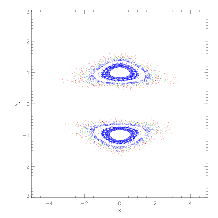
Figure 3: Surface of section of orbits at effective energy value of -1, from the $bar+sp_{18}$ model. The strongly chaotic orbits are in medium grey shading, while the regular orbits are in the darkest shade. The intermediate shading corresponds to the weakly chaotic orbits.

As for the overall bimodal character of the local phase space, a rudimentary orbital analysis confirms that in line with the Kalnajs Mechanism, the overall bimodality is indeed due to scattering off $OLR_{b}$; the Hercules stream appears to be built of quasi-periodic orbits belonging to the anti-aligned family while the anti-aligned family was not spotted in the other larger mode. (The other mode manifests orbits from the aligned family).

6 The Role of Chaos

fux_aa has suggested bar-induced chaos as the cause for the local streams. However, in a chaos quantification exercise that is currently underway (Chakrabarty $\&$ Sideris, submitted to A$\&$A), the orbits in the $bar-only$ model are found to be regular; it is noted that it is the presence of the spiral that triggers the onset of chaos. Figure 3 indicates the relative fraction of chaotic orbits, over regular and weakly chaotic orbits, in the $bar+sp_{18}$ models. Similar surfaces of section for the $bar-only$ models, at even higher energies indicate no irregularity.

It is of course possible that a stronger bar would induce greater irregularity than in our work, but the point is that the local phase space structure can be emulated with the bar strength used herein.

7 Summary $\&$ Future Work

In this contribution, we have attempted to understand the state of the local phase space via dynamical modelling that includes the influence of the bar and the spiral pattern in the Galaxy. The clumpy structure of the 2-D local velocity distribution was attributed to the major and minor resonances of these perturbations, as well as the emergence of chaoticity triggered primarily by the spiral potential. Only the models that take the gravitational potentials of both bar and spiral are found to offer viable representations of the Solar neighbourhood dynamics; overlap of the results from the successful models indicate a fast bar, with a pattern speed of 57.4${}^{+3.0}_{-2.5}$ km s^-1 kpc^-1and a bar angle that lies in the range [0^∘, 30^∘].

The currently used $p$-value formalism is not satisfactory on account of the lack of automativeness and inability to rank or grade the models. In fact, we are hoping to improve upon this technique, with a Bayesian measure of the quality of a simulation. This is to aid the expansion of the relevant parameter space, particularly, in the inclusion of the effects of the halo and progression to a full six dimensional phase space.

References

- (1) Woolley, R.: The Observatory, 81, 203 (1961)
- (2) A. J. Kalnajs: Pattern Speeds of Density Waves. In Dynamics of Disk Galaxies, ed by B. Sundelius (Göetberg, Sweden 1991) pp.323.
- (3) Dehnen, W. and Binney, J.: Monthly Notices of the Royal Astronomical Society, 298, 387 (1998).
- (4) Fux, R.: Astrophysical Journal, 373, 511 (2001).
- (5) Skuljan, J., Hearnshaw, J. B. and Cottrell, P. L.: Monthly Notices of the Royal Astronomical Society, 308, 731 (1999).
- (6) Dehnen, W.: Astronomical Journal, 119, 800 (2000).
- (7) De Simone, R., Wu, X. and Tremaine, S.: Monthly Notices of the Royal Astronomical Society, 350, 627 (2004).
- (8) Quillen, A. C.: Astrophysical Journal, 125, 785 (2003).
- (9) Famaey, B., Jorissen, A., Luri, X., Mayor, M., Udry, S., Dejonghe, H. and Turon, C.: Astronomy Astrophysics, 430, 165 (2005).
- (10) Chakrabarty, D.: Astronomy Astrophysics, 467, 145, (2007).
- (11) Kaufmann, D. E., & Contopoulos, G.: Astronomy Astrophysics, 309, 381 (1996)
- (12) Boonyasait, V., Patsis, P. A., & Gottesman, S. T.: New York Academy Sciences Annals, 1045, 2 (2005)
- (13) Evans, N. W. and Read, J. C. A.: Monthly Notices of the Royal Astronomical Society, 300, 83 (1998).
- (14) Bissantz, N. and Englmaier, P. and Gerhard, O.: Monthly Notices of the Royal Astronomical Society, 340, 949 (2003).
- (15) Melnik, A.: Astronomy Letters, 32, 7 (2006).
- (16) Johnston, S., Koribalski, B., Weisberg, J. M. and Wilson, W., Monthly Notices of the Royal Astronomical Society, 322 , 715 (2001).