Trading Model with Pair Pattern Strategies

Abstract

A simple trading model based on pair pattern strategy space with holding periods is proposed. Power-law behaviors are observed for the return variance $\sigma^{2}$, the price impact $H$ and the predictability $K$ for both models with linear and square root impact functions. The sum of the traders’ wealth displays a positive value for the model with square root price impact function, and a qualitative explanation is given based on the observation of the conditional excess demand $\langle A|u\rangle$. An evolutionary trading model is further proposed, and the elimination mechanism effectively changes the behavior of the traders highly performed in the model without evolution. The trading model with other types of traders, e.g., traders with the MG’s strategies and producers, are also carefully studied.

,

1 Introduction

The standard Minority Game (MG) introduced and studied by Challet and Zhang cha97 , zha98 was initially designed as a simplification of Arthur’s famous El Farol’s Bar problem art94 . It describes a system in which many heterogeneous traders adaptively compete for a scarce resource, and it captures some key features of a generic market mechanism and the basic interaction between the traders and public information. However, it is a highly simplified model, not suitable to compare with real financial market trading. To make it more realistic in comparison with the real markets, different variations cha01 , jef00 , cha01a , gia02 , and02 , MGw04 , ren06 of the standard MG are consequently proposed. For example, the inactive strategy is introduced, which grants the traders with the possibility of not trading and thus the number of traders actively trading at each time step varies throughout the game. This type of extension is called the grand canonical MG, and it produces the main characteristics of the stock markets, e.g., the ”fat tail” return distribution and the long-range volatility correlations.

In the standard MG and most of its variations, the strategies give predictions for the next time step based on the current state of the history, and upon which traders make instantaneous trading action with an horizon not more than one time step. For example, the MG-based models with dynamic capitals jef00 , cha01a , in which the wealth of the traders is updated according to the current trading price and has no relation with the trades they have made previously. The payoff raised from the price change at the next time step is grant to the trader immediately after a single trade. In fact traders have asset holding periods and make profits from price difference between two consecutive trading actions of buying and selling in the real stock markets. To find a strategy space with holding periods, that traders open or close their positions and hold their positions reasonably is a great challenge for modeling speculation.

Recently, a new model based on a simple pattern-based strategy space with holding periods is proposed by Challet cha08 . In this model, the strategy space is composed of a sequence of patterns, i.e., history signals. Traders open or close positions when the current pattern is the pattern listed in the strategy space, and hold positions between patterns. The kind of position he/she might take, i.e., buying or selling is determined by the average price return between two consecutive occurrences of patterns. The explicitly trading action of buying or selling is not fixed with the patterns. A simplest case that the strategy space consists of only one pair of patterns is mainly considered.

Inspired from Challet’s work, we introduce a new pattern-based speculation model in which the patterns strategy space is split into several sub-spaces composed by pairs of patterns. Different from Challet’s model, we defined the explicitly trading actions of the pair patterns. One strategy consists of a pair of patterns, which denote the history signals for buying and selling. It is reasonable to assume that the trader base their decisions on patterns or history signals since they may have some experiences and know when to buy or sell according to the history signals. The order of the pair patterns does not make any sense, which means the position can be opened by buying/selling if the history signal for buying/selling comes first. Therefore, the trader should buy first if he/she wants to sell, or buy only after he/she sells in this model. That is exactly the case in the real stock markets.

The MG is a negative sum game due to the minority essence of its payoffs. The traders compete for the limited market resource and only those traders in the minority group are rewarded. Challet’s new model keeps the minority-game payoffs impacted by his/her own trades when the trader opens and close the position. Furthermore, it introduces a new term of majority-game payoffs raised from the contribution of other traders during his/her holding periods. The sum of the payoffs therefore depends on the trading frequency and reaction time of each trader, and thus makes the dynamics relatively complicated.

For the real financial market, the sum of the social wealth should be positive due to the general increase of the social productivity. Traders are willing to trade in the market which has a positive sum of the social wealth or at least has a zero sum. The purpose of this paper is to construct a model with holding periods which has a zero sum or positive sum. We first assume a zero wealth sum in our model by introducing a simple mid-price dynamics with a linear price impact function. Furthermore, a square root impact function revealed by the empirical study of the real stock market ple02 , gab03 , has91 is considered, and the model consequently tends to be a positive sum game. The payoff for each trader is naturally determined by the difference between the selling price and the buying price. We name this model as trading model due to the trading essence of the pair patterns.

In Sec. II, we first introduce a pattern-based speculation model by Challet, and then introduce our trading model with pair pattern strategies. A comprehensive comparison between the definition of the strategy space and the payoffs of our model and that of Challet’s model is detailed presented. Some numerical results of our trading model are subsequently presented. In Sec. III, a dynamic evolution mechanism is introduced to the trading model, and the process how the traders are washed out and how their wealth evolves are carefully studied. In Sec. IV, other types of traders are introduced to the trading model, and Sec. V contains the conclusion.

2 Trading Model with Pattern-based Strategy Space

2.1 A pattern-based speculation model by Challet

The model proposed by Challet cha08 consists of N traders, and they base their decisions on patterns. Each trader $i$ is able to recognize $S$ patterns $\mu_{i,1},\cdot\cdot\cdot,\mu_{i,S}$, drawn randomly and uniformly from $\{1,\cdot\cdot\cdot,P\}$ at the beginning of the game and kept fixed throughout the game. Each trader $i$ keeps track of the cumulative price return between two consecutive occurrences of patterns, denoted by $U_{i,\mu\rightarrow\nu}$, where $\mu,\nu\in\mu_{i,1},\cdot\cdot\cdot,\mu_{i,S}$ and $\mu\neq\nu$. At time $t$, the trader may wish to open position only when the current history signal $\mu(t)$ is in his pattern list, that is, $\mu(t)\in\{\mu_{i,1},\cdot\cdot\cdot,\mu_{i,S}\}$. The kind of position he/she might take, $a_{i}(t)=0,\pm 1$ denoting inactive, buying and selling, is determined by average price return between two consecutive occurrences of patterns: if $|U_{i,\mu\rightarrow\nu}(t)|>\epsilon t_{\mu\rightarrow\nu}$, where $t_{\mu\rightarrow\nu}$ is the total number of time-steps between patterns $\mu$ and $\nu$ and $\epsilon>0$ is a parameter, one buys a share ($U_{i,\mu\rightarrow\nu}(t)>0$) or sells a share ($U_{i,\mu\rightarrow\nu}(t)<0$), and then hold his/her position until $\mu(t^{\prime})=\nu$. The excess demand is $A(t)=\sum_{i=1}^{N}a_{i}(t)$. A linear price impact function is considered, and thus the price return is simply defined as

$$r(t)=p(t+1)-p(t)=A(t).$$ (1)

Assume that $\mu(t_{\mu})=\mu$ and $t_{\nu}$ is the first subsequent occurrence of pattern $\nu$, the cumulative price return $U_{i,\mu\rightarrow\nu}$ between pattern $\mu$ and $\nu$ evolves according to

$$U_{i,\mu\rightarrow\nu}(t_{\nu}+1)=U_{i,\mu\rightarrow\nu}(t_{\mu}) + p(t_{\nu}+1)-p(t_{\mu}+1)$$ (2)

$$- (1-|a_{i}(t_{\mu})|)\zeta_{i}[A(t_{\nu})-A(t_{\mu})],$$

where $\zeta_{i}$ is a naivety factor indicating the reaction time of trader $i$. By adjusting the value of the parameters $\epsilon$ and $\zeta_{i}$, we observe that the model exhibits a withdraw phenomena in its price evolution.

If trader $i$ decides to open a position at time $t_{i,\mu}$ and close his/her position at time $t_{i,\nu}$, then his/her payoff is

$$a_{i}[p(t_{i,\nu}+\delta t_{i,\nu})-p(t_{i,\mu}+\delta t_{i,\mu})]= - a_{i}A(t_{i,\mu},\delta t_{i,\mu})+a_{i}\sum_{t_{i,\mu}+\delta t_{i,\mu}<t\leq t_{i,\nu}}a(t)$$ (3)

$$- (-a_{i})A(t_{i,\nu},\delta t_{i,\nu}),$$

$$A(t_{i,\mu},\delta t_{i,\mu})=\sum_{t_{i,\mu}<t\leq t_{i,\mu}+\delta t_{i,\mu}}a(t).$$ (4)

$\delta t_{i,\mu}$ and $\delta t_{i,\nu}$ are one’s reaction time when he/she opens and closes position, which may due to communication delays and the time needed to make a conscious decision. The first and the last terms are minority-game payoffs, which can be easily recognize by their ’-’ sign: the trader is rewarded if he/she takes an action opposite to the majority of the orders executed during the time delay. The central term which has a ’+’ sign could be regarded as a delayed majority-game payoff: the trader is rewarded if he/she takes an action consequently proved to be consistent with the majority of the orders executed during the holding period. Therefore, the traders’ wealth depends on the situation of the market: the relative importance of minority games decreases as the trading frequency decreases and increases as the reaction time of each trader increases.

2.2 Trading model with pair pattern strategies

The trading model takes the form of a repeated game with a certain number of traders $N$. Different from challet’s model, we split the pattern strategy space into several sub-spaces in units of pair patterns. A strategy consists of a pair of patterns or history signals with explicit trading actions, labeled as $(\mu,\nu)$, where $\mu$ is for buying and $\nu$ is for selling. A pattern or history signal records the possible status of the $m$ most recent outcomes of the price change. Since there are a total of $2^{m}$ possible patterns and the patterns of one strategy should not repeat, there are a total of $2^{m}*(2^{m}-1)$ probable pairs of patterns.

At the beginning of the game, each trader randomly picks $S$ strategies from the full strategy space and keep them fixed throughout the game. Each trader $i$ keeps track of the cumulative performance of his/her pair pattern strategy $s,s=1,...,S$ by assigning a virtual score $U_{i,s}$ to it. The initial scores of the strategies are set to be zero. At time $t$, each trader $i$ adopts the strategy with the highest score $s_{i}(t)$, and checks if either of the two patterns of the highest score strategy is consistent with the history at that moment. If the pattern for buying occurs first, the trader opens an position by buying and holds the position until the pattern for selling occurs. Then the trader closes the position by selling. The trader can also open the position by selling if the pattern for seeling occurs first and then close the position by buying. Therefore, the model is symmetric. The action will then be $a_{i}(t)=0,\pm 1$, denotes inactive, buying and selling. The excess demand is defined as $A(t)=\sum\limits_{i=1}^{N}a_{i}(t)$.

We define a simple price dynamics of returns with a linear price impact function the same as Eq. (1). Assuming that one of the patterns of a strategy occurs at time $t_{1}$ and $t_{2}$ is the first subsequent occurrence of the other pattern, the score of the strategy is updated according to the price difference between these two patterns as

$$U_{i,s}(t_{2}+1)=U_{i,s}(t_{1})+p(t_{s_{i},\nu}+1)-p(t_{s_{i},\mu}+1),$$ (5)

where $s_{i}$ is the strategy of trader $i$. If the pattern for buying $\mu$ occurs first $t_{s_{i},\mu}=t_{1}$ and $t_{s_{i},\nu}=t_{2}$, and if the pattern for selling $\nu$ occurs first $t_{s_{i},\nu}=t_{1}$ and $t_{s_{i},\mu}=t_{2}$. Therefore, the payoff of the strategy is determined by the profit made from the strategy if it is adopted. In our model, we assume the traders are sophisticated and compute perfectly the price return, and this makes Eq. (5) look like Eq. (2) with $\zeta_{i}=0$.

A wealth $W_{i}$ is assigned to each trader $i$. If trader $i$ decides to open a position at time $t_{1}$ and closes it at time $t_{2}$, the wealth is updated according to the price return between these two trades as

$$W_{i}(t_{2}+1)=W_{i}(t_{1})+p(t_{i,{\nu}}+1)-p(t_{i,{\mu}}+1).$$ (6)

If the trader opens a position by buying first $t_{i,{\mu}}=t_{1}$ and $t_{i,{\nu}}=t_{2}$, and if the trader opens a position by selling first $t_{i,{\nu}}=t_{1}$ and $t_{i,{\mu}}=t_{2}$.

However, the model with payoffs defined as above is a negative-sum game, which means that the sum of the wealth of all the traders is negative. Considering the simplest case that the market only has one trader, the payoff of his/her wealth is always $-1$ no matter what kind of position he/she might take first. We assume that the model with linear price impact function has a nature of zero-sum. Inspired by the works in Refs.and02 , far98 , a middle price is introduced $p(t^{\prime}+1)=\frac{1}{2}(p(t+1)+p(t))$. Supposing that not all the shares are executed at the price immediately after the trades, the traders make trades at the middle price on average. The price return defined with the linear price impact function is

$$r(t^{\prime})=p(t^{\prime}+1)-p(t^{\prime})=\frac{1}{2}(A(t^{\prime})+A(t^{\prime}-1)),$$ (7)

where $A(t^{\prime})=A(t)$. The score of the strategy and the wealth of each trader are consequently updated according to the middle price, replacing $t$ by $t^{\prime}$ in Eqs. (5) and (6). We simply assume that the trader has no reaction time, and therefore the payoff looks like Eq. (3) with $\delta t=0$. The sum of the traders’ wealth at time $t^{\prime}$ is

$$\sum_{i}W_{i}(t^{\prime})=\sum_{i}\sum_{t^{\prime}_{i,1},t^{\prime}_{i,2}}^{1\leq t^{\prime}_{i,1},t^{\prime}_{i,2}\leq t^{\prime}}[\frac{1}{2}A(t^{\prime}_{i,1})+\frac{1}{2}A(t^{\prime}_{i,2})+\sum_{t^{\prime}_{i,1}<\tau<t^{\prime}_{i,2}}A(\tau)],$$ (8)

where $t^{\prime}_{i,1}$ is the time trader $i$ opens a position and $t^{\prime}_{i,2}$ is the time trader $i$ closes it. For the model with line price impact function, the sum of the first two terms approximately equals zero since the number of positions opened by traders equals to that closed by traders. The sum of the traders’ wealth consequently depends on the cumulative access demand contributed by the traders during the holding periods.

Recent empirical study shows that the volume imbalance seems to have a square root impact on the price return ple02 , gab03 , has91 . Therefore, we also introduce a square root impact function to the price return as

$$r(t^{\prime})=p(t^{\prime}+1)-p(t^{\prime})=\frac{1}{2}(sign(A(t^{\prime}))\sqrt{|A(t^{\prime})|}+sign(A(t^{\prime}-1))\sqrt{|A(t^{\prime}-1)|}).$$ (9)

The score of the strategy, the wealth of each trader and the sum of the traders’ wealth are consequently updated according to this price dynamics.

2.3 The results

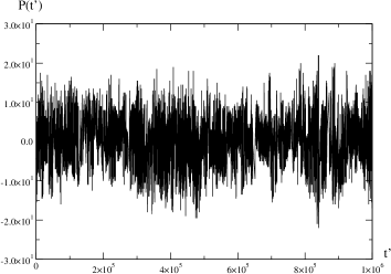
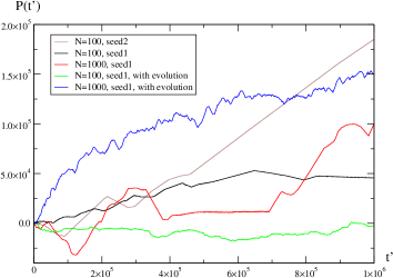
Figure 1: (a) Price evolution of the trading model with linear price impact function at $N=100$, $S=2$ and $m=3$. (b) Price evolution of the trading model with square root price impact function for different values of the parameter $N$ and different initial seeds at $S=2$ and $m=3$. $10^{6}$ data are collected after $500$ iterations for equilibrium.

Numerous numerical simulations are performed for this trading model with pair pattern strategies, and the results for $S=2$ and $m=3$ are mainly reported. The price evolution of the trading model with linear price impact function for $N=100$, and square root price impact function for $N=100,1000$ and different initial seeds are plotted in Fig. 1(a) and (b). For the model with linear price impact function, the curve for $N=100$ fluctuates symmetrically around zero, and the curve for other value of the parameter $N$ behaves similar to that of $N=100$ (not shown in figure). For the model with square root price impact function, it seems that the price fluctuates similar to that of the financial markets. However, we observe some attractors for some singular runs, for example the curve for $N=100$ with $seed2$ changes suddenly close to $t^{\prime}=5.0*10^{5}$ and then the system stuck in a string of periodical history states which may leads to the abnormal increase of the price.

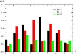
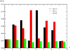
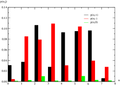
Figure 2: Conditional probability $p(u,j)$ of the model with linear price impact function for: (a) $N=50$, (b) $N=100$, (c) $N=1000$ at $S=2$ and $m=3$.

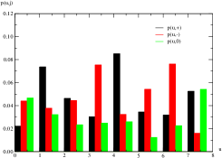
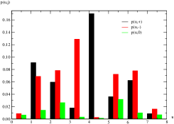
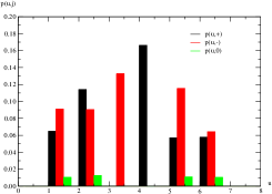
Figure 3: Conditional probability $p(u,j)$ of the model with linear price impact function for: (a) $N=50$, (b) $N=100$, (c) $N=1000$ at $S=2$ and $m=3$.

We first compute the conditional probability $p(u,j)$, which is the conditional probability to have positive, negative and zero price change, denoted by $j=\pm 1,0$, immediately following a specific history $u$. In Fig. 2(a), (b) and (c), $p(u,j)$ for the trading model with linear price impact function for $N=50,100,1000$ are plotted. In general, the histograms are not as flat as that of the MG model sav99 which means the model has a bias of price change conditional to a specific history. We observe that the histogram for larger $N$ is less flat than the histogram for smaller $N$, which means the price has a relative strong biased tendency at large values of the parameter $N$. In Fig. 3(a), (b) and (c), $p(u,j)$ for the trading model with square root price impact function for $N=50,100,1000$ are plotted. The curves for the model with square root price impact function is less flat than those of the model with linear price impact function.

The variance of returns is a convenient reciprocal measure of the market fluctuation, and it is defined as

$$\sigma^{2}=\frac{<r^{2}>-<r>^{2}}{P}.$$ (10)

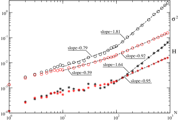
Figure 4: Variance of returns $\sigma^{2}$ (circles) and price impact $H$ (stars) for the trading models with linear and square root price impact functions at $S=2$ and $m=3$, represented by black and red symbols respectively. The results take average over $100$ runs.

The smaller $\sigma^{2}$ is, the less the return fluctuates. In Fig. 4, the variance $\sigma^{2}$ for the trading models with linear and square root price impact functions are plotted, denoted by black and red circles respectively. $\sigma^{2}$ for the model with linear price impact function increases as the increase of the parameter $N$, and obeys power laws with exponents $0.79$ for $N\in[10,100)$ and $1.81$ for $N\in[100,1000)$. $\sigma^{2}$ for the model with square root price impact function obeys power laws with exponents $0.59$ for $N\in[10,100)$, and $0.92$ for $N\in[100,1000)$. Compared with the model with linear price impact function, the model with square root price impact function has a smaller magnitude of the price fluctuation though it has a stronger biased tendency of the price change.

To further understand the price return bias conditional to the market states, we compute the average return conditional to a given history defined as

$$H=\frac{\sum_{u}\langle r|u\rangle^{2}}{P}.$$ (11)

In Fig. 4, $H$ for the trading models with linear and square root price impact functions are also plotted, denoted by black and red stars respectively. $H$ increases as the increase of the parameter $N$, displaying a behavior similar to that of $\sigma^{2}$. $H$ for the model with linear price impact function seems saturated and fluctuates slightly for $N\in[10,100)$, then obeys a nice power law with an exponent $1.64$ for $N\in[100,1000)$. $H$ for the model with square root price impact function obeys a power law with an exponent $0.95$ for $N\in[100,1000)$. These two exponents are close to the half of the exponents of their price impact functions, which indicates $H$ can be considered as an approximate measure of the average price impact for large values of the parameter $N$.

Another important variable is the predictability that the traders hope to exploit from the pair patterns

$$K=\frac{1}{P(P-1)}\sum_{\mu,\nu,\mu\neq\nu}\langle r(t)|\mu\rightarrow\nu\rangle^{2},$$ (12)

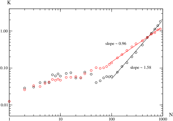
Figure 5: Predictability $K$ for the trading models with linear and square root price impact functions at $S=2$ and $m=3$, represented by black and red circles respectively. The results take average over $100$ runs.

where $\langle r(t)|\mu\rightarrow\nu\rangle$ stands for the average price return per time step between the occurrence of $\mu$ at time $t$ and the next occurrence of $\nu$. In Fig. 5, the predictability $K$ for the model with linear and square root price impact functions are plotted. For the model with linear price impact function, $K$ increases at the early stage of the parameter $N$, and shows an unclear behavior due to the unneglectable oscilation for $N\in[10,100)$, then follows a power-law behavior with an exponent $1.58$ for $N\in[100,1000)$. For the model with square root price impact function, $K$ is a monotonously increasing function of the parameter $N$, and obeys a power law with an exponent $0.96$ for $N\in[100,1000)$. The model with square root price impact function is more predictable than the model with linear price impact function for $N\in[40,400]$, and tends to be less predictable if we further increase the parameter $N$.

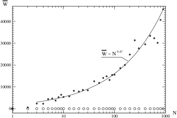
Figure 6: Average wealth for each trader for the trading models with linear and square root price impact functions at $S=2$ and $m=3$, represented by circles and stars respectively. The solid line is the fitting curve $\overline{W}\sim N^{0.47}$.

We then consider the wealth of the traders. The average wealth for each trader $\overline{W}=\frac{\sum_{i}W_{i}}{N}$ is calculated. In Fig. 6, the average wealth for each trader for different values of the parameter $N$ at $t^{\prime}=10^{6}$ are plotted. The circles and stars are for the trading models with linear and square root price impact functions respectively. The average wealth for the model with linear price impact function is close to zero independent of the parameter $N$, which indicates that the system is a zero-sum game. Remarkably, the model with square root price impact displys a positive wealth sum: the curve increases as the increase of the parameter $N$ and can be nicely fitted by a power law with an exponent $0.47$.

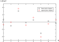
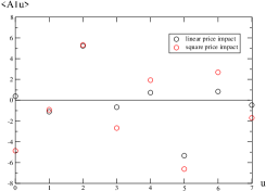
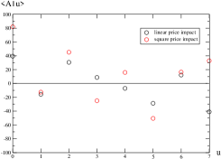
Figure 7: Excess demand bias $\langle A|u\rangle$ for the trading models with linear and square root price impact functions for: (a) $N=50$, (b) $N=100$, (c) $N=1000$ at $S=2$ and $m=3$.

To understand why the trading model with linear price impact function displays a zero sum and the trading model with square root price impact function displays a positive sum, we further investigate the average excess demand bias $\langle A|u\rangle$ conditional to a specific history $u$. In Fig. 7 (a), (b) and (c), $\langle A|u\rangle$ for the trading models with linear and square root price impact functions (represented by black and red circles respectively) for $N=50,100,1000$ are plotted. For the model with linear price impact function, the sum of the trader’s wealth mainly depends on the cumulative access demand contributed by the traders during the holding periods according to Eq. (8). Assuming that the game visits each possible history with a equal probability, so the sum over $\tau$ between two consecutive actions of opening and closing a position could be substituted by the sum over the possible history states between them. $\langle A|u\rangle$ for trading model with linear price impact function is symmetrically distributed above and below zero for different states of history $u$. $|\sum_{u}\langle A|u\rangle|$ displays a value close to zero. Therefore, we observe a zero wealth sum.

The sum of the traders’ wealth for the model with square root price impact function mainly depends on the cumulative square root impact of the access demand contributed by the traders during the holding periods, supposing that the sum of the square root impact of the excess demand at which the traders open and close their positions equals zero, i.e., $\sum_{i}\sum_{t^{\prime}_{i,1},t^{\prime}_{i,2}}^{1\leq t^{\prime}_{i,1},t^{\prime}_{i,2}\leq t^{\prime}}[\frac{1}{2}sign(t^{\prime}_{i,1})\sqrt{A(t^{\prime}_{i,1})}+\frac{1}{2}sign(A(t^{\prime}_{i,2}))\sqrt{A(t^{\prime}_{i,2})}]=0$, where $t^{\prime}_{i,1}$ is the time trader $i$ opens a position and $t^{\prime}_{i,2}$ is the time trader $i$ closes it. $\langle A|u\rangle$ for the model with square root price impact function is unsymmetrically distributed above and below zero. $|\sum_{u}\langle A|u\rangle|$ displays a nonzero value obviously larger than that of the model with linear price impact function, e.g., the ratio of $|\sum_{u}\langle A|u\rangle|$ between two models with square root and linear price impact functions is $7.56,18.58,62.66$ for $N=50,100,1000$ . The larger the parameter $N$ is, the more unsymmetrical the distribution of $\langle A|u\rangle$ is. Some traders have certain strategies which can help them to effectively exploit the information of the biased excess demand from the patterns, and they make profits from these high-performed strategies. They have wealth greater than zero while other traders have an average wealth close to zero. This may leads to a positive sum for the model with square root impact function.

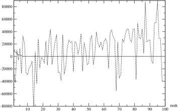
Figure 8: (a) Wealth distribution of traders and change frequency of adopted strategies for the model with square root price impact function for $N=100$ at $S=2$ and $m=3$, represented by dashed and solid lines separately. (b) Wealth distribution and age of traders for the trading model with evolution for $N=1000$ at $S=2$ and $m=3$, represented by dashed and solid lines separately.

In Fig. 8 (a), the wealth distribution of the traders for the model with square root price impact function for $N=100$ is plotted according to the rank of their change frequency of the adopted strategies. We observe that the traders who change their strategies more frequently have less wealth. Some traders keep using their high-performed strategies to make more profits, while the others who do not have these strategies always shift among their strategies and have less wealth. Especially for some singular runs with attractors, we observe that some traders keep using certain high-performed strategies and the others shift among their strategies at the early stage of the evolution and eventually withdraw from the market and thus the system is stuck in a string of period history states. For the model with linear price impact function, the wealth distribution shows a similar behavior but displays a zero sum.

3 Trading Model with Evolution

MG-based models with dynamic evolution have been studied in Refs. sys03 , li00 , cha01a . For example, in Refs. sys03 , li00 the traders can change their strategies with poor performances. In this trading model, we assume that the worst trader can be driven out of the market following Ref cha01a . Every 100 time steps the trader who has the lowest wealth is washed out and a new trader with new randomly selected strategies is generated. The wealth of the new trader is set to be the average wealth of the traders at that moment. We use the square root price impact function of the real markets in this evolutionary trading model. With this evolution mechanism, the price evolution becomes more continuously, and seems to be similar to that of the real markets as it is shown in Fig. 1.

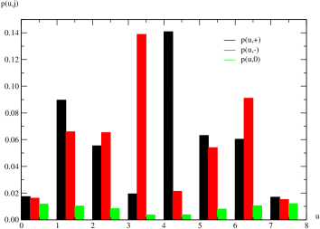
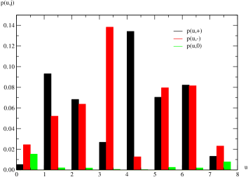
Figure 9: Conditional probability $p(u,j)$ of the trading model with evolution for: (a) $N=100$, (b)$N=1000$ at $S=2$ and $m=3$.

The conditional probability $p(u,j)$ for different values of the parameter $N=100,1000$ for this evolutionary trading model are plotted in Fig. 9 (a) and Fig. 9 (b). It seems that the histograms of the model with evolution are more flat than those of the model without evolution for the same values of the parameter $N$. The introduction of the elimination mechanism leads to a relatively week biased tendency of the price change. $\sigma^{2}$, $H$ and $K$ for the evolutionary model are also effectively decreased. In general, the elimination mechanism breaks down the domination of the strategies highly performed in the trading model and makes the price fluctuations relatively symmetric.

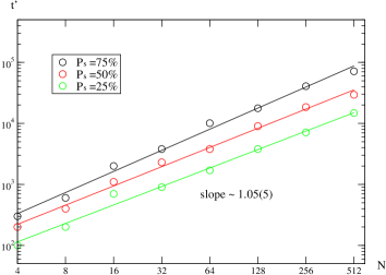
Figure 11: Time $t^{\prime}$ at which $P_{s}$ percentage of the traders are washed out for the trading model with evolution at $S=2$ and $m=3$.

In Fig. 10, the number of the traders still survive evolved with time $t^{\prime}$ is plotted. For a large number of traders, e.g., $N=1000$, those traders who have the strategy (2,5) could survive for quite a long time and are finally washed out one after another in a short time region. There is no high-performed strategy always keep winning after we introduce the elimination mechanism. We also observe that the time at which the traders are washed out mainly depends on the parameter $N$. Fig. 11 shows the time $t^{\prime}$ at which $P_{s}$ percentage of the traders are washed out as a function of the parameter $N$. $t^{\prime}$ increases as the increase of the parameter $N$, and obeys a power law with an exponent close to $1.05$ not much different for different values of the parameter $P_{s}=25\%,50\%,75\%$.

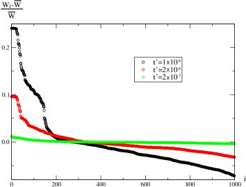
Figure 12: Relative wealth distribution $(W_{i}{t^{\prime}}-\overline{W})/\overline{W}$ at different time $t^{\prime}=1\times 10^{6},2\times 10^{6},2\times 10^{7},5\times 10^{7}$ for the trading model with evolution at $S=2$, $m=3$ and $N=1000$.

Let’s take a look at how the traders’ wealth evolve before they are washed out. In Fig. 12, the distribution of the relative wealth $(W_{i}(t^{\prime})-\overline{W})/\overline{W}$ at different time $t^{\prime}=1\times 10^{6},2\times 10^{6},2\times 10^{7}$ are plotted, where $i$ is the rank of the trader’s wealth and $\overline{W}$ is the average wealth of the traders at time $t^{\prime}$. For $t^{\prime}=1\times 10^{6}$, the relative wealth is not continuous distributed among the traders. Those traders who have higher wealth are clustered in different groups. For $t^{\prime}=2\times 10^{6}$, the distribution remains similar, but the relative wealth difference between the rich traders and the poor traders is not so large and thus the curve becomes more flat. At the time just before all the traders are washed out, e.g., $t^{\prime}=2\times 10^{7}$, the relative wealth distribution becomes even more flat.

The wealth distribution of the traders ranked by their age (survival time) for the trading model with evolution is plotted in Fig. 8 (b). We observe that all the traders have positive wealth due to the evolution mechanism. Those elder traders have relatively more wealth than those younger traders, and those traders newly generated have an average wealth among them. In Fig. 13, the return distributions of the models with and without evolution for a single run are plotted. Though the return distributions of both models decay exponentially, the model with evolution has a tail fatter than the model without evolution.

4 Trading Model with Other Types of Traders

We introduce the traders who have the strategies the same as those in the MG model cha97 , zha98 , which give the predictions for all the probable history status, to the trading model with square root price impact function but without evolution. Each of these newly introduced traders has the same number of $S$ randomly selected strategies, and they trade at each time step using their best strategies according to the pattern (or history) shared by all the traders. Let $N_{t}$ and $N_{m}$ be the number of the traders who have the pair pattern strategies and who have the strategies the same as those in the MG model. Then the excess demand is defined as $A(t)=\sum_{i=1}^{N_{t}+N_{m}}a_{i}(t)$, and the price dynamics remains the same as Eq. (9). The score of the pair pattern strategy takes the same update form as Eq. (5), and the score of the MG’s strategy is updated as $U_{i,s}(t^{\prime}+1)=U_{i,s}(t^{\prime})-a_{i}(t^{\prime})(P(t^{\prime}+1)-P(t^{\prime}))$, $i=1,...,N_{m}$.

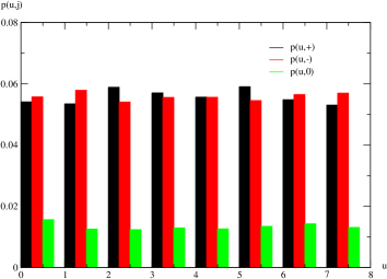
Figure 14: Conditional probability $p(u,j)$ for the trading model with mixed population $N_{t}=100$ and $N_{m}=25$ at $S=2$ and $m=3$.

The conditional probability $p(u,j)$ and the wealth distribution of the traders ranked by their change frequency of the adopted strategies for $N_{t}=100$ and $N_{m}=25$ are plotted in Fig. 14 and Fig. 15 (a). The number of the traders effectively trade at each time step ${N_{t}}_{eff}:{N_{m}}_{eff}=1:1$. The histogram of the conditional probability becomes much more flat than that of the model has pure traders who have the pair pattern strategies, and the sum of the wealth of the traders who have the pair pattern strategies tends to be negative. The traders who have the MG’s strategies distinctly affect the behavior of the traders who have the pair pattern strategies.

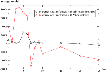
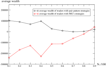
Figure 16: Average wealth of the traders who have the pair pattern strategies and average wealth of the traders who have the MG’s strategies for the trading model with mixed population: (a) $N_{m}$ ranging from 1 to 25 at fixed $N_{t}=100$, (b) different proportion of $N_{t}/100$ at fixed $N_{t}+N_{m}=100$ for $S=2$ and $m=3$.

We fix the number of the traders who have the pair pattern strategies $N_{t}=100$, and increase the number of the traders who have the MG’s strategies one by one and see how the traders’ wealth behave. In Fig. 16 (a), the average wealth of the traders who have the pair pattern strategies and the traders who have the MG’s strategies for $N_{m}$ ranging from 1 to 25 at fixed $N_{t}=100$ are plotted. For a small $N_{m}$, the average wealth of the traders who have the MG’s strategies is positive and larger than that of the traders who have pair pattern strategies. Few number of the traders dominant the game, and are fed by the rest majority traders who have positive wealth sum. Interestingly, at $N_{m}\sim 5$ the average wealth of both types of traders reaches a maximum. Those two types of traders seem to have a certain state of corporation. As we further increase $N_{m}$, the average wealth of the traders who have the MG’s strategies tends to be negative and smaller than that of the traders who have pair pattern strategies.

Another case that the total number of the traders is fixed is also considered, i.e., $N_{t}+N_{m}=100$. We change the proportion of $N_{t}$ to the total number of the traders. In Fig. 16 (b), the average wealth of both types of traders are plotted for fixed $N_{t}+N_{m}=100$. The average wealth of the traders who have the MG’s strategies increases with the increase of the proportion of $N_{t}/100$, while the average wealth of the traders who have the pair pattern strategies decreases with the increase of the proportion of $N_{t}/100$. For a small $N_{t}/100$, the average wealth of the traders who have the MG’s strategies is negative and smaller than that of the traders who have the pair pattern strategies, and tends to be positive and larger than that of the traders who have the pair pattern strategies for $N_{t}/100\sim 0.9$. That is consistent with the result we obtained for fixed $N_{t}=100$ shown in Fig. 16 (a).

We also introduce the traders who only have one MG’s strategy known as ”producers” cha01 to the trading model with square root price impact function but without evolution. As it is shown in Fig. 15 (b), the introduce of this type of traders can effectively increase the wealth of the traders who have the pair pattern strategies. Most of the traders who have the pair pattern strategies have positive wealth, but the wealth distribution is more fluctuated than the model with the traders who have the MG’s strategies shown in Fig. 15 (a).

5 Conclusion

In summary, trading model with pair pattern strategies evolved with middle price is introduced. Both linear price impact function and empirical square root impact function are considered in the price dynamics, and power-law behaviors are observed for the return variance $\sigma^{2}$, the price impact $H$ and the predictability $K$ at the large values of the parameter $N$. The sum of the traders’ wealth displays a positive value for the trading model with square root price impact function. An unsymmetrically distribution of the conditional excess demand $\langle A|u\rangle$ is observed, and based on this observation we give a qualitative explanation for the positive wealth sum for the model with square root price impact function. In addition, an evolution mechanism is introduced to the trading model. The introduction of new traders with randomly selected strategies breaks down the domination of the strategies highly performed in the model without evolution, and leads to a relatively small value for the biased tendency of the price change, as well as $\sigma^{2}$, $H$ and $K$. Power-law behavior is observed for the time $t^{\prime}$ at which $P_{s}$ percentage of the traders are washed out, and the relative wealth difference between the rich and poor traders becomes much smaller when the time approaches the point that all the traders are washed out. The traders with the MG’s strategies are also introduced to the trading mode. The small friction of the mixed traders are fed by the rest majority of traders, and thus have relatively more wealth. We also introduce the traders known as producers to this trading model, and find it leads to an effectively increase of the traders’ wealth.

Acknowledgments:

During this work, we have enjoyed the support and hospitality of ISI, Torino, Italy and Renmin Univ, Beijing, China.

Figure 10: Number of traders still survive evolves with time $t^{\prime}$ for the trading model with evolution at $S=2$, $m=3$, and $N=1000$.

Figure 13: Return distribution of the trading models with and without evolution for $S=2$, $m=3$ and $N=1000$, represented by red and black lines separately.

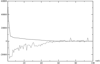
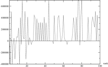
Figure 15: Wealth distribution and the change frequency of the adopted strategies of the traders who have the pair pattern strategies for the trading model with mixed population: (a) $N_{t}=100$ and $N_{m}=25$, (b) $N_{t}=100$ and $N_{p}=100$ (the number of the traders known as producers) at $S=2$ and $m=3$, represented by dashed and solid lines separately.

References

- [1] D. Challet, Y.-C. Zhang, Emergence of cooperation and organization in an evolutionary game 246 (1997) 407–418.
- [2] Y.-C. Zhang, Modeling market mechanism with evolutionary games, Europhys. News 29 (1998) 51–54.
- [3] W. B. Arthur, Inductive reasoning and bounded rationality 84 (1994) 406–411.
- [4] D. Challet, M. Marsili, Y.-C. Zhang, Stylized facts of financial markets and market crashes in minority games 294 (2001) 514–524.
- [5] P. Jefferies, M. L. Hart, P. M. Hui, N. F. Johnson, From market games to real-world markets 20 (2001) 493–501.
- [6] D. Challet, M. Chessa, A.and Marsili, Y.-C. Zhang, From minority games to real markets 1 (2001) 168–176.
- [7] I. Giardina, J.-P. Bouchaud, Bubbles, crashes and intermittency in agent based market models 31 (2003) 421–437.
- [8] J. V. Andersen, D. Sornette, The $-game 31 (2003) 141–145.
- [9] See the Minority Game’s web page on http://www.unifr.ch/econophysics/minority.
- [10] F. Ren, B. Zheng, T. Qiu, S. Trimper, Minority games with score-dependent and agent-dependent payoffs 74 (2006) 041111.
- [11] D. Challet, Inter-pattern speculation: Beyond minority, majority and $-games 32 (2008) 85–100.
- [12] V. Plerou, P. Gopikrishnan, X. Gabaix, H. E. Stanley, Quantifying stock-price response to demand fluctuations 66 (2002) 027104.
- [13] X. Gabaix, P. Gopikrishnan, V. Plerou, H. E. Stanley, A Theory of Power-Law Distributions in Financial Market Fluctuations, Nature 423 (2003) 267–270.
- [14] J. Hasbrouck, Measuring the information content of stock trades 46 (1991) 179–207.
- [15] J. D. Farmer, Market force, ecology and evolution, Industrial and Corporate Change 11 (2002) 895–953.
- [16] R. Savit, R. Manuca, R. Riolo, Adaptive competition, market efficiency, and phase transitions 82 (1999) 2203–2206.
- [17] M. Sysi-Aho, A. Chakraborti, K. Kaski, Adaptation using hybridized genetic crossover strategies 322 (2003) 701–709.
- [18] Y. Li, R. Riolo, R. Savit, Evolution in minority games. (I). Games with a fixed strategy space 276 (2000) 234–264.