On some difficulties with a posterior probability approximation technique

Abstract

In Scott (2002) and Congdon (2006), a new method is advanced to compute posterior probabilities of models under consideration. It is based solely on MCMC outputs restricted to single models, i.e., it is bypassing reversible jump and other model exploration techniques. While it is indeed possible to approximate posterior probabilities based solely on MCMC outputs from single models, as demonstrated by Gelfand and Dey (1994) and Bartolucci et al. (2006), we show that the proposals of Scott (2002) and Congdon (2006) are biased and advance several arguments towards this thesis, the primary one being the confusion between model-based posteriors and joint pseudo-posteriors. From a practical point of view, the bias in Scott’s (2002) approximation appears to be much more severe than the one in Congdon’s (2006), the latter being often of the same magnitude as the posterior probability it approximates, although we also exhibit an example where the divergence from the true posterior probability is extreme.

0.1 Introduction

Model selection is a fundamental statistical issue and a clear asset of the Bayesian methodology but it faces severe computational difficulties because of the requirement to explore simultaneously the parameter spaces of all models under comparison accurately enough to provide sufficient approximations to the posterior probabilities of all models. When Green (1995) introduced reversible jump techniques, it was perceived by the community as the second MCMC revolution in that it allowed for a valid and efficient exploration of the collection of models and the subsequent literature on the topic exploiting reversible jump MCMC is a testimony to the appeal of this method. Nonetheless, the implementation of reversible jump techniques in complex situations may face difficulties or at least inefficiencies of its own and, despite some recent advances in the devising of the jumps underlying reversible jump MCMC (Brooks et al., 2003), the care required in the construction of those jumps often acts as a deterrent from its applications.

There are practical alternatives to reversible jump MCMC when the number of models under consideration is small enough to allow for a complete exploration of those models. Integral approximations using importance sampling techniques like those found in Gelfand and Dey (1994), based on a harmonic mean representation of the marginal densities, and in Gelman and Meng (1998), focussing on the optimised selection of the importance function, are advocated as potential solutions, see Chen et al. (2000) for a detailed introduction. The reassessment of those methods by Bartolucci et al. (2006) showed the connection between a virtual reversible jump MCMC and importance sampling (see also Chopin and Robert, 2007). In particular, those papers demonstrated that the output of MCMC samplers on each single model could be used to produce approximations of posterior probabilities of those models, via some importance sampling methodologies also related to Newton and Raftery (1994).

In Scott (2002) and Congdon (2006), a new and straightforward method is advanced to compute posterior probabilities of models under scrutiny based solely on MCMC outputs restricted to single models. While this simplicity is quite appealing for the approximation of those probabilities, we believe that both proposals of Scott (2002) and Congdon (2006) are inherently biased and we advance in this note several arguments towards this thesis. In addition, we notice that, to overcome the bias we thus exhibited, a valid solution would call for the joint simulation of parameters under all models (using priors or pseudo-priors) and, in this step, the primary appeal of the methods would thus be lost compared to the one proposed by Carlin and Chib (1995), from which both Scott (2002) and Congdon (2006) are inspired.

We want to point out at this stage that the original purpose of Scott (2002) is to provide a survey of Bayesian methods for the analysis of hidden Markov models and thus that the approximation we analyse here is introduced as a side remark within the whole paper. If we insist here on the bias produced by Scott’s (2002) approximation, it is because it generated followers, including Congdon (2006), and because both approximations are based on the same erroneous interpretation of the marginal distribution in Bayesian model choice. We also note that Congdon’s (2006) approximation often produces values that are numerically of the same magnitude as the true value of the posterior probabilities, with sometimes very close proximity as illustrated in Example 2 of Section 0.3.4, but also potential severe mishaps as in Example 4 of Section 0.3.4.

0.2 The methods

In a Bayesian framework of model comparison (see, e.g., Robert, 2001), given $D$ models in competition, $\mathfrak{M}_{k}$, with densities $f_{k}(y|\theta_{k})$, and prior probabilities $\varrho_{k}=P(M=k)$ $(k=1,\ldots,D)$, the posterior probabilities of the models $\mathfrak{M}_{k}$ conditional on the data $y$ are given by

$$P(M=k|y)\propto\varrho_{k}\,\int f_{k}(y|\theta_{k})\pi_{k}(\theta_{k})\,\text{d}\theta_{k}\,,$$

the proportionality term being given by the sum of the above and $M$ denoting the unknown model index.

In the specific setup of hidden Markov models, the solution of Scott (2002, Section 4.1) is to generate, simultaneously and independently, $D$ MCMC chains

$$(\theta_{k}^{(t)})_{t}\,,\qquad 1\leq k\leq D\,,$$

with stationary distributions $\pi_{k}(\theta_{k}|y)$ and to approximate $P(M=k|y)$ by

$$\tilde{\varrho}_{k}(y)\propto\varrho_{k}\sum_{t=1}^{T}\left\{f_{k}(y|\theta_{k}^{(t)})\bigg{/}\sum_{j=1}^{D}\varrho_{j}\,f_{j}(y|\theta_{j}^{(t)})\right\}\,,$$

as reported in formula (21) of Scott (2002), with the indication that (21) averages the $D$ likelihoods corresponding to each $\theta_{j}$ over the life of the Gibbs sampler (p.347), the latter being understood as independently sampled $D$ parallel Gibbs samplers (p.347).

Adopting a more general perspective, the proposal of Congdon (2006) for an approximation of the $P(M=k|y)$’s follows both from Scott’s (2002) approximation and from the pseudo-prior construction of Carlin and Chib (1995) that predated reversible jump MCMC by saturating the parameter space with an artificial simulation of all parameters at each iteration. However, due to a very special (and, we believe, mistaken) choice of pseudo-priors discussed below, Congdon’s (2006, p.349) approximation of $P(M=k|y)$ eventually reduces to the estimator

$$\hat{\varrho}_{k}(y)\propto\varrho_{k}\sum_{t=1}^{T}\left\{f_{k}(y|\theta_{k}^{(t)})\pi_{k}(\theta^{(t)}_{k})\bigg{/}\sum_{j=1}^{D}\varrho_{j}\,f_{j}(y|\theta_{j}^{(t)})\pi_{j}(\theta^{(t)}_{j})\right\}\,,$$

where the $\theta_{k}^{(t)}$’s are samples from $\pi_{k}(\theta_{k}|y)$ (or approximate samples obtained by an MCMC algorithm). This is a simple and readily implementable formula that attracted other researchers like Chen et al. (2008).

Although both approximations $\tilde{\varrho}_{k}(y)$ and $\hat{\varrho}_{k}(y)$ clearly differ in their expressions, by the addition of a $\pi_{k}(\theta^{(t)}_{k})$ term in Congdon’s (2006) formula, they fundamentally relate to the same notion that parameters from other models can be ignored when conditioning on the model index $M$. This approach is therefore bypassing the simultaneous exploration of several parameter spaces and it restricts the simulation effort to marginal samplers on each separate model. This feature is very appealing since it cuts most of the complexity from the schemes both of Carlin and Chib (1995) and of Green (1995). We however question the foundations of those approximations as presented in both Scott (2002) and Congdon (2006) and advance below arguments that both authors are using incompatible versions of joint distributions on the collection of parameters that jeopardise the validity of the approximations.

0.3 Difficulties

The sections below expose the difficulties found with both methods, following the arguments advanced in Scott (2002) and Congdon (2006), respectively. The fundamental difficulty with both approaches appears to us to stem from a confusion between the model dependent simulations and the joint simulations based on a pseudo-prior scheme as in Carlin and Chib (1995). Once this difficulty is resolved, it appears that the corresponding approximation of $P(M=k|y)$ by $\hat{P}(M=k|y)$ does require a joint simulation of all parameters and thus that the solutions proposed in Scott (2002) and Congdon (2006) are of the same complexity as the proposal of Carlin and Chib (1995). If single models MCMC chains are to be used, alternative approaches described for instance in Chen et al. (2000) and compared in Gamerman and Lopes (2006) can be implemented.

0.3.1 Incorrect marginals

We denote by $\theta=\left(\theta_{1},\ldots,\theta_{D}\right)$ the collection of parameters for all models under consideration. Both Scott (2002) and Congdon (2006) start from the representation

$$P(M=k|y)=\int P(M=k|y,\theta)\pi(\theta|y)\,\text{d}\theta$$

to justify the approximation

$$\hat{P}(M=k|y)=\sum_{t=1}^{T}P(M=k|y,\theta^{(t)})/T\,.$$

This is indeed an unbiased estimator of $P(M=k|y)$ provided the $\theta^{(t)}$’s are generated from the correct (marginal) posterior

$$\pi(\theta|y) =\sum_{k=1}^{D}P(\theta,M=k|y)$$ (1)

$$\propto\sum_{k=1}^{D}\varrho_{k}\,f_{k}(y|\theta_{k})\prod_{j}\pi_{j}(\theta_{j})$$

$$=\sum_{k=1}^{D}\varrho_{k}\,m_{k}(y)\,\pi_{k}(\theta_{k}|y)\prod_{j\neq k}\pi_{j}(\theta_{j})\,.$$ (2)

In both papers, the $\theta^{(t)}$’s are instead simulated as independent outputs from the componentwise posteriors $\pi_{k}(\theta_{k}|y)$ and this divergence jeopardises the theoretical validity of the approximation. The error in both interpretations stems from the fact that, while the $\theta^{(t)}_{k}$’s are (correctly) independent given the model index $M$, this independence does not hold once $M$ is integrated out, which is the case for the $\theta^{(t)}_{k}$’s in the above approximation $\hat{P}(M=k|y)$.

0.3.2 MCMC versus marginal MCMC

When Congdon (2006) defines a Markov chain $(\theta^{(t)})$ at the top of page 349, he indicates that the components of $\theta^{(t)}$ are made of independent Markov chains $(\theta_{k}^{(t)})$ simulated with MCMC samplers related to the respective marginal posteriors $\pi_{k}(\theta_{k}|y)$, following the approach of Scott (2002). The aggregated chain $(\theta^{(t)})$ is thus stationary against the product of those marginals,

$$\prod_{k=1}^{D}\pi_{k}(\theta_{k}|y)\,.$$

However, in the derivation of Carlin and Chib (1995), the model is defined in terms of (1) and the Markov chain should thus be constructed against (1), not against the product of the model marginals. Obviously, in the case of Congdon (2006), the fact that the pseudo-joint distribution does not exist because of the flat prior assumption (see Section 0.3.3 for a proof) prevents this construction but, in the case the flat prior is replaced with a proper (pseudo-) prior, the same statement holds: the probabilistic derivation of $P(M=k|y)$ relies on the pseudo-prior construction and, to be valid, it does require the completion step at the core of Carlin and Chib (1995), where parameters need to be simulated from the pseudo-priors. Generating from the component-wise posteriors $\pi_{k}(\theta_{k}|y)$ produces a bias.

Similarly, in Scott (2002), the target of the Markov chain $(\theta^{(t)},M^{(t)})$ should be the distribution

$$P(\theta,M=k|y)\propto\pi_{k}(\theta_{k})\,\varrho_{k}\,f_{k}(y|\theta_{k})\,\prod_{j\neq k}\pi_{j}(\theta_{j})$$

and the $\theta_{j}^{(t)}$’s should thus be generated from the prior $\pi_{j}(\theta_{j})$ when $M^{(t)}\neq j$—or equivalently from the corresponding marginal if one does not condition on $M^{(t)}$, but simulating a Markov chain with stationary distribution (2) is certainly a challenge in many settings if the latent variable decomposing the sum is not to be used.

Since, in both Scott (2002) and Congdon (2006), the $(\theta^{(t)})$’s are not simulated against the correct target, the resulting averages of $P(M=k|y,\theta^{(t)})$, $\tilde{\varrho}_{k}(y)$ and $\hat{\varrho}_{k}(y)$, will both be biased, as demonstrated in the examples of Section 0.3.4.

0.3.3 Improperty of the posterior

When resorting to the construction of pseudo-posteriors adopted by Carlin and Chib (1995), Congdon (2006) uses a flat prior as pseudo-prior on the parameters that are not in model $\mathfrak{M}_{k}$. More precisely, the joint prior distribution on $(\theta,M)$ is given by Congdon’s (2006) formula (2),

$$P(\theta,M=k) =\pi_{k}(\theta_{k})\,\varrho_{k}\,\prod_{j\neq k}\pi(\theta_{j}|M=k)$$

$$=\pi_{k}(\theta_{k})\,\varrho_{k}\,,$$

which is indeed equivalent to assuming a flat prior as pseudo-prior on the parameters $\theta_{j}$ that are not in model $\mathfrak{M}_{k}$.

Unfortunately, this simplifying assumption has a dramatic consequence in that the corresponding joint posterior distribution of $\theta$ is never defined (as a probability distribution) since

$$\pi(\theta|y)=\sum_{k=1}^{D}\pi_{k}(\theta_{k}|y)\,P(M=k|y)$$

does not integrate to a finite value in any of the $\theta_{k}$’s (unless their support is compact). While Congdon (2006) states that it is not essential that the priors for $P(\theta_{j\neq k}|M=k)$ are improper (p.348), the truth is that they cannot be improper.

The fact that the posterior distribution on the saturated vector $\theta=(\theta_{1},\ldots,\theta_{D})$ does not exist obviously has negative consequences on the subsequent derivations, since a positive recurrent Markov chain with stationary distribution $\pi(\theta|y)$ cannot be constructed. Similarly, the fact that

$$P(M=k|y)=\int P(\theta,M=k|Y)\,\text{d}\theta$$

does not hold any longer.

Note that Scott (2002) does not follow the same track: when defining the pseudo-priors in his formula (20), he uses the product definition

$$P(\theta,M=k)=\pi_{k}(\theta_{k})\,\varrho_{k}\,\prod_{\scriptstyle j\neq k}\pi_{j}(\theta_{j})\,,\\$$

which means that the true priors could also be used as pseudo-priors across all models. However, we stress that Scott (2002) does not refer to the construction of Carlin and Chib (1995) in his proposal, nor does he use pseudo-priors in his simulations.

0.3.4 Illustrations

We now proceed through several toy examples where all posterior quantities can be computed in order to evaluate the bias induced by both approximations and we observe that, despite its theoretical bias, Congdon’s (2006) can sometimes achieve a close approximation of the posterior probability, but also that, in other settings, it may produce an unreliable evaluation.

Example 1.

Consider the case when a model $\mathfrak{M}_{1}:\,y|\theta\sim\mathcal{U}(0,\theta)$ with a prior $\theta\sim\mathcal{E}xp(1)$ is opposed to a model $\mathfrak{M}_{2}:\,y|\theta\sim\mathcal{E}xp(\theta)$ with a prior $\theta\sim\mathcal{E}xp(1)$. We also assume equal prior weights on both models: $\varrho_{1}=\varrho_{2}=0.5$.

The marginals are then

$$m_{1}(y)=\int_{y}^{\infty}\theta^{-1}e^{-\theta}\,\text{d}\theta=\text{E}_{1}(y)\,,$$

where $\text{E}_{1}$ denotes the exponential integral function tabulated both in Mathematica and in the GSL library, and

$$m_{2}(y)=\int_{0}^{\infty}\theta e^{-\theta(y+1)}\,\text{d}\theta=\frac{1}{(1+y)^{2}}\,.$$

For instance, when $y=0.2$, the posterior probability of $\mathfrak{M}_{1}$ is thus equal to

$$P(M=1|y) =m_{1}(y)/\{m_{1}(y)+m_{2}(y)\}$$

$$=\text{E}_{1}(y)/\{\text{E}_{1}(y)+(1+y)^{-2}\}$$

$$\approx 0.6378\,,$$

while, for $y=0.9$, it is approximately $0.4843$. This means that, in the former case, the Bayes factor of $\mathfrak{M}_{1}$ against $\mathfrak{M}_{2}$ is $B_{12}\approx 1.760$, while for the latter, it decreases to $B_{12}\approx 0.939$.

The posterior on $\theta$ in model $\mathfrak{M}_{2}$ is a gamma $\mathcal{G}a(2,1+y)$ distribution and it can thus be simulated directly. For model $\mathfrak{M}_{1}$, the posterior is proportional to $\theta^{-1}\,\exp(-\theta)$ for $\theta$ larger than $y$ and it can be simulated using a standard accept-reject algorithm based on an exponential $\mathcal{E}xp(1)$ proposal translated by $y$.

Using simulations from the true (marginal) posteriors and the approximation of Congdon (2006), the numerical value of $\hat{\varrho}_{1}(y)$ based on $10^{6}$ simulations is $0.7919$ when $y=0.2$ and $0.5633$ when $y=0.9$, which translates into Bayes factors of $3.805$ and of $1.288$, respectively. For the approximation of Scott (2002), the numerical value of $\tilde{\varrho}_{1}(y)$ is $0.6554$ (corresponding to a Bayes factor of $1.898$) when $y=0.2$ and $0.6789$ when $y=0.9$ (corresponding to a Bayes factor of $2.11$), based on the same simulations. Note that in the case $y=0.9$, a selection based on either approximation of the Bayes factor would select the wrong model.

If we use instead a correct simulation from the joint posterior (2), which can be achieved by using a Gibbs scheme with target distribution $P(\theta,M=k|y)$, we then get a proper MCMC approximation to the posterior probabilities by the $\hat{P}(M=k|y)$’s. For instance, based on $10^{6}$ simulations, the numerical value of $\hat{P}(M=1|y)$ when $y=0.2$ is $0.6370$, while, for $y=0.9$, it is $0.4843$. Note that, due to the impropriety difficulty exposed in Section 0.3.3, the equivalent correction for Congdon’s (2006) scheme cannot be implemented.

In Figure 1, the three approximations are compared to the exact value of $P(M=1|y)$ for a range of values of $y$. The correct simulation produces a graph that is indistinguishable from the true probability, while Congdon’s (2006) approximation stays within a reasonable range of the true value and Scott’s (2002) approximation drifts apart for most values of $y$. $\blacktriangleleft$

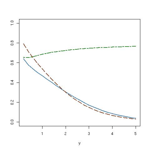
Figure 1: Example 1: Comparison of three approximations of $P(M=1|y)$ with the true value (in blue and full lines): Scott’s (2002) approximation (in green and mixed dashes), Congdon’s (2006) approximation (in brown and dashes), while the correction of Scott’s (2002) approximation is indistinguishable from the true value (based on $N=10^{6}$ simulations).

The above correspondence of what is essentially Carlin and Chib’s (1995) scheme with the true numerical value of the posterior probability is obviously unsurprising in this toy example but more advanced setups see the approximation degenerate, since the simulations from the prior are most often inefficient, especially when the number of models under comparison is large. This is the reason why Carlin and Chib (1995) introduced pseudo-priors that were closer approximations to the true posteriors.

The proximity of Congdon’s (2006) approximation with the true value in Figure 1 shows that the method could possibly be used as a cheap first-order substitute of the true posterior probability if the bias was better assessed. First, we note that when all the componentwise posteriors are close to Dirac point masses at values $\hat{\theta}_{k}$, Congdon’s (2006) approximation is close to the true value

$$\hat{\varrho}_{k}(y)\approx\varrho_{k}f_{k}(y|\hat{\theta}_{k})\pi_{k}(\hat{\theta}_{k})\bigg{/}\sum_{j=1}^{D}\left\{\varrho_{j}\,f_{j}(y|\hat{\theta}_{j})\pi_{j}(\hat{\theta}_{j})\right\}\,.$$

Further, the posterior expectation of $f_{k}(y|\theta_{k}^{(t)})\pi_{k}(\theta^{(t)}_{k})$ involves the integral of

$$\int\frac{f_{k}(y|\theta_{k})^{2}\pi_{k}(\theta_{k})^{2}}{m_{k}(y)}\,\,\text{d}y\,,$$

thus the bias is likely to be small in settings where the product $f_{k}(y|\theta_{k}^{(t)})\pi_{k}(\theta^{(t)}_{k})$ is peaked as in large samples, for instance. That the bias can almost completely disappear is exposed through a second toy example.

Example 2.

Consider the case when a normal model $\mathfrak{M}_{1}:\,y\sim\mathcal{N}(\theta,1)$ with a prior $\theta\sim\mathcal{N}(0,1)$ is opposed to a normal model $\mathfrak{M}_{2}:\,y\sim\mathcal{N}(\theta,1)$ with a prior $\theta\sim\mathcal{N}(5,1)$. We again assume equal prior weights.

In that case, the marginals are available in closed form

$$m_{1}(y)=\frac{1}{\sqrt{4\pi}}\,\exp-\frac{y^{2}}{4}\quad\text{and}\quad m_{2}(y)=\frac{1}{\sqrt{4\pi}}\,\exp-\frac{(y-5)^{2}}{4}$$

and the posterior probability of model $\mathfrak{M}_{1}$ is

$$P(M=1|y)=\left\{1+\exp\frac{5(2y-5)}{4}\right\}^{-1}\,.$$

For argumentation’s sake, assume that we now produce both sequences $(\theta_{1}^{(t)})$ and $(\theta_{2}^{(t)})$ from the posterior distributions $\mathcal{N}(y/2,1/2)$ and $\mathcal{N}((y+5)/2,1/2)$, respectively, by using the same sequence of $\epsilon_{t}\sim\mathcal{N}(0,1)$, i.e.

$$\theta_{1}^{(t)}=\frac{y}{2}+\frac{1}{\sqrt{2}}\epsilon_{t}\quad\text{and}\quad\theta_{2}^{(t)}=\frac{y+5}{2}+\frac{1}{\sqrt{2}}\epsilon_{t}\,.$$

Using those sequences, we then obtain that

$$\frac{\exp-\frac{1}{2}(y-\theta_{1}^{(t)})^{2}-\frac{1}{2}(\theta_{1}^{(t)})^{2}}{\exp-\frac{1}{2}(y-\theta_{2}^{(t)})^{2}-\frac{1}{2}(\theta_{2}^{(t)}-5)^{2}} =\frac{\exp-\frac{1}{2}(y-\frac{y}{2}-\frac{1}{\sqrt{2}}\epsilon_{t})^{2}-\frac{1}{2}(\frac{y}{2}+\frac{1}{\sqrt{2}}\epsilon_{t})^{2}}{\exp-\frac{1}{2}(y-\frac{y+5}{2}-\frac{1}{\sqrt{2}}\epsilon_{t})^{2}-\frac{1}{2}(\frac{y+5}{2}+\frac{1}{\sqrt{2}}\epsilon_{t}-5)^{2}}$$

$$=\frac{\exp-\frac{1}{2}(\frac{y}{2}-\frac{1}{\sqrt{2}}\epsilon_{t})^{2}-\frac{1}{2}(\frac{y}{2}+\frac{1}{\sqrt{2}}\epsilon_{t})^{2}}{\exp-\frac{1}{2}(\frac{y-5}{2}-\frac{1}{\sqrt{2}}\epsilon_{t})^{2}-\frac{1}{2}(\frac{y-5}{2}+\frac{1}{\sqrt{2}}\epsilon_{t})^{2}}$$

$$=\exp-\frac{5}{4}(2y-5)\,,$$

independently of $\epsilon_{t}$, and thus that Congdon’s (2006) approximation is truly exact using this device! Figure 2 shows the difference due to using two independent sequences of $10^{4}$ $\epsilon_{t}$’s [instead of one single sequence] and the severe discrepancy resulting from Scott’s approximation. (Note that using an artificial MCMC sampler in this case would only increase the variability of the approximations.)

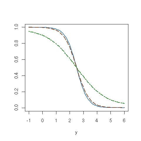
Figure 2: Example 2: Comparison of two approximations of $P(M=1|y)$ with the true value (in blue and full lines): Scott’s (2002) approximation (in green and mixed dashes) and Congdon’s (2006) approximation (in brown and long dashes) (based on $N=10^{4}$ simulations).

$\blacktriangleleft$

The approximation may also be rather crude, as shown in the following example, inspired from an example posted on Peter Congdon’s web-page in connection with Congdon (2007).

Example 3.

Consider comparing $\mathfrak{M}_{1}:\,y\sim\mathcal{B}(n,p)$ when $p\sim\mathcal{B}e(1,1)$ with $\mathfrak{M}_{2}:\,y\sim\mathcal{B}(n,p)$ when $p\sim\mathcal{B}e(m,m)$. Once again, the posterior probability can be computed in closed form since the Bayes factor is given by

$$B_{12}=\frac{(n+1)!}{y!(n-y)!}\,\frac{(m+y-1)!(m+n-y-1)!}{(m+n-1)!}\,\frac{(m-1)!^{2}}{(2m-1)!}\,.$$

The simulations of $p_{1}^{(t)}$ from the posterior $\mathcal{B}e(y+1,n-y+1)$ in model $\mathfrak{M}_{1}$ and of $p_{2}^{(t)}$ from the posterior $\mathcal{B}e(y+m,m+n-y)$ in model $\mathfrak{M}_{2}$ are straightforward (and obviously do not require an extra MCMC step). Figure 3 shows the impact of Congdon’s (2006) approximation on the evaluation of the posterior probability for $n=15$ and $m=100$: the magnitude is the same but, in that case, the numerical values are quite different.

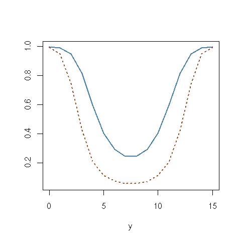
Figure 3: Example 3: Comparison of Congdon’s (2006) (in brown and dashed lines) approximation of $P(M=1|y)$ with the true value (in blue and full lines) when $n=15$ and $m=510$ (based on $N=10^{4}$ simulations).

In the case of three models in competition, namely when $y\sim\mathcal{B}(n,p)$ and the three priors are $p\sim\mathcal{B}e(1,1)$, $p\sim\mathcal{B}e(a,b)$ and $p\sim\mathcal{B}e(c,d)$, the differences may be of the same order, as shown in Figure 4, but the discrepancy is nonetheless decreasing with the sample size $n$.

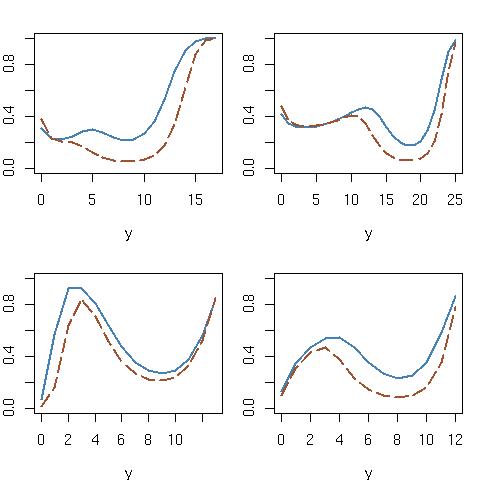
Figure 4: Example 3: Comparison of Congdon’s (2006) (in brown and dashed lines) approximation of $P(M=1|y)$ with the true value (in blue and full lines) when $(n,a,b,c,d)$ is equal to $(17,2.5,12.5,501.5,500)$, $(25,1.5,4,540,200)$, $(13,.5,100.5,20,10)$ and $(12,.3,1.8,200,200)$, respectively (based on $N=10^{4}$ simulations).

$\blacktriangleleft$

At last, the approximation may fall very far from the mark, as demonstrated in the following example where the approximation has an asymptotic behaviour opposite to the one of the true posterior probability.

Example 4.

Consider comparing $\mathfrak{M}_{1}:\,y\sim\mathcal{N}(0,1/\omega)$ with $\omega\sim\mathcal{E}xp(a)$ against $\mathfrak{M}_{2}:\,\exp(y)\sim\mathcal{E}xp(\lambda)$ with $\lambda\sim\mathcal{E}xp(b)$. The corresponding marginals are given in closed form by

$$m_{1}(y)=\int_{0}^{\infty}\sqrt{\frac{\omega}{2\pi}}\,e^{-(y^{2}/2)\omega}\,ae^{-a\omega}\,\text{d}\omega=\frac{a}{\sqrt{2\pi}}\,\frac{\Gamma(3/2)}{(a+y^{2}/2)^{3/2}}$$

and

$$m_{2}(y)=\int_{0}^{\infty}e^{y}\,\lambda e^{-e^{y}\lambda}\,be^{-b\lambda}\,\text{d}\lambda=\frac{b\,e^{y}}{(b+e^{y})^{2}}\,.$$

The associated posteriors are $\omega|y\sim\mathcal{G}a(3/2,a+y^{2}/2)$ and $\lambda|y\sim\mathcal{G}a(2,b+e^{y})$. Figure 5 shows the comparison of the true posterior probability of $\mathfrak{M}_{1}$ with the approximation for various values of $(a,b)$ and it indicates a very poor fit when $y$ goes to $+\infty$.

It is actually possible to show that the approximation always converges to $0$ when $y$ goes to $+\infty$, while the true posterior probability goes to $1$. Indeed, when $y$ goes to $+\infty$, the Bayes factor is

$$\frac{m_{1}(y)}{m_{2}(y)}\approx\frac{a\Gamma(3/2)}{b\sqrt{2\pi}}\,\frac{e^{2y}}{e^{y}(y^{2}/2)^{3/2}}\,,$$

which goes to $+\infty$ while, since $\omega^{(t)}=\epsilon_{t}/(a+y^{2}/2)$ and $\lambda^{(t)}=\upsilon_{t}/(b+e^{y})$, with $\epsilon_{t}\sim\mathcal{G}(3/2,1)$ and $\upsilon_{t}\sim\mathcal{G}(2,1)$,

$$\frac{f_{1}(y|\omega^{(t)})\pi_{1}(\omega^{(t)})}{f_{2}(y|\lambda^{(t)})\pi_{2}(\lambda^{(t)})}=\frac{a}{b\sqrt{2\pi}}\,\frac{\sqrt{\epsilon_{t}}e^{-\epsilon_{t}}}{\upsilon_{t}e^{-\upsilon_{t}}}\,\frac{b+e^{y}}{e^{y}(a+y^{2}/2)^{1/2}}\approx\frac{a}{b\sqrt{2\pi}}\,\frac{\sqrt{\epsilon_{t}}e^{-\epsilon_{t}}}{\upsilon_{t}e^{-\upsilon_{t}}}\,\frac{\sqrt{2}}{y}\,,$$

which goes to $0$ for all $(\epsilon_{t},\upsilon_{t})$. The discrepancy is then extreme.

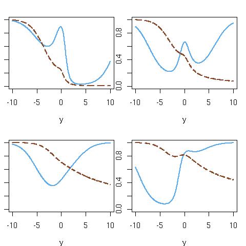
Figure 5: Example 4: Comparison of Congdon’s (2006) (in brown and dashed lines) approximation of $P(M=1|y)$ with the true value (in blue and full lines) when $(a,b)$ is equal to $(.24,8.9)$, $(.56,.7)$, $(4.1,.46)$ and $(.98,.081)$, respectively (based on $N=10^{4}$ simulations).

$\blacktriangleleft$

References

- Bartolucci et al. (2006) Bartolucci, F., L. Scaccia, and A. Mira. 2006. Efficient Bayes factor estimation from the reversible jump output. Biometrika 93: 41–52.
- Brooks et al. (2003) Brooks, S., P. Giudici, and G. Roberts. 2003. Efficient construction of reversible jump Markov chain Monte Carlo proposal distributions (with discussion). J. Royal Statist. Society Series B 65(1): 3–55.
- Carlin and Chib (1995) Carlin, B. and S. Chib. 1995. Bayesian model choice through Markov chain Monte Carlo. J. Royal Statist. Society Series B 57(3): 473–484.
- Chen et al. (2008) Chen, C., R. Gerlach, and M. So. 2008. Bayesian Model Selection for Heteroskedastic Models. Advances in Econometrics 23. To appear.
- Chen et al. (2000) Chen, M., Q. Shao, and J. Ibrahim. 2000. Monte Carlo Methods in Bayesian Computation. Springer-Verlag, New York.
- Chopin and Robert (2007) Chopin, N. and C. Robert. 2007. Contemplating Evidence: properties, extensions of, and alternatives to Nested Sampling. Tech. Rep. 2007-46, CEREMADE, Université Paris Dauphine. ArXiv:0801.3887.
- Congdon (2006) Congdon, P. 2006. Bayesian model choice based on Monte Carlo estimates of posterior model probabilities. Comput. Stat. Data Analysis 50: 346–357.
- Congdon (2007) —. 2007. Model weights for model choice and averaging. Statistical Methodology 4(2): 143–157.
- Gamerman and Lopes (2006) Gamerman, D. and H. Lopes. 2006. Markov Chain Monte Carlo. 2nd ed. Chapman and Hall, New York.
- Gelfand and Dey (1994) Gelfand, A. and D. Dey. 1994. Bayesian model choice: asymptotics and exact calculations. J. Royal Statist. Society Series B 56: 501–514.
- Gelman and Meng (1998) Gelman, A. and X. Meng. 1998. Simulating normalizing constants: From importance sampling to bridge sampling to path sampling. Statist. Science 13: 163–185.
- Green (1995) Green, P. 1995. Reversible jump MCMC computation and Bayesian model determination. Biometrika 82(4): 711–732.
- Newton and Raftery (1994) Newton, M. and A. Raftery. 1994. Approximate Bayesian inference by the weighted likelihood boostrap (with discussion). J. Royal Statist. Society Series B 56: 1–48.
- Robert (2001) Robert, C. 2001. The Bayesian Choice. 2nd ed. Springer-Verlag, New York.
- Scott (2002) Scott, S. L. 2002. Bayesian methods for hidden Markov models: recursive computing in the 21st Century. J. American Statist. Assoc. 97: 337–351.