Polarization and frequency disentanglement of photons via stochastic polarization mode dispersion

Abstract

We investigate the quantum decoherence of frequency and polarization variables of photons via polarization mode dispersion in optical fibers. By observing the analogy between the propagation equation of the field and the Schrödinger equation, we develop a master equation under Markovian approximation and analytically solve for the field density matrix. We identify distinct decay behaviors for the polarization and frequency variables for single-photon and two-photon states. For the single photon case, purity functions indicate that complete decoherence for each variable is possible only for infinite fiber length. For entangled two-photon states passing through separate fibers, entanglement associated with each variable can be completely destroyed after characteristic finite propagation distances. In particular, we show that frequency disentanglement is independent of the initial polarization status. For propagation of two photons in a common fiber, the evolution of a polarization singlet state is addressed. We show that while complete polarization disentanglement occurs at a finite propagation distance, frequency entanglement could survive at any finite distance for gaussian states.

I Introduction

Polarization mode dispersion (PMD) in optical fibers limits fiber performance when designing optical channels with high bit rate PMD_review . Physically, the origin of PMD is optical birefringence caused by the asymmetry of the fiber due to factors such as external mechanical stress and temperature fluctuations, resulting in different group velocities for two orthogonal polarization modes. In addition, stochastic optical birefringence inside a single mode fiber leads to the random coupling of the two polarization modes, thus causing effects such as pulse widening PMD_review ; Agrawal , and the fluctuations of arrival times of pulses grow with the square root of the propagation distance Gisin1995 . Existing major applications of quantum communication, including quantum cryptography quancryp and quantum teleportation teleport ; teleportexpt , rely on quantum entanglement between photons as a crucial element. Therefore strategies to cope with decoherence have been investigated recently, for example, protection schemes based on decoherence-free subspace (DFS) have been proposed DFSDuan ; DFS1 ; DFS2 ; Konrad . Typically, a decoherence free two-photon state involves polarization singlet states with both photons having the same frequency singletexpt . However, it is known that for photons with different frequencies, decoherence by PMD cannot be avoided due to the breaking of symmetry of the collective states limitations .

Entangled photon pairs produced by spontaneous down-conversion can be hyperentangled hyperent ; hyperexpt , i.e. entangled in various degrees of freedom (DOFs) of the photons. For example, polarization hypershih ; hyperzy , frequency hyperfreq , angular momentum hyperam1 ; hyperam2 , and energy time energytime are variables that can be exploited. It is thus important to address how quantitatively hyperentangled photons disentangle for each DOF, by investigating the decoherence of each DOF separately. In this paper, we focus on polarization and frequency hyperentangled photons and explore how the entanglement of these two DOFs may affect each other inside optical fibers with stochastic PMD.

The main purpose of this paper is to determine disentanglement length scales associated with frequency and polarization variables due to PMD decoherence, and to quantify the residual entanglement as photons propagate. To this end we will investigate three situations of photon propagation as depicted in Fig. 1. First we examine the propagation of single photon states, then hyperentangled two-photon states, in both polarization and frequency DOFs. In one case we consider each photon passes through separate fibers, and in another case both photons pass through the same fiber, all of length $L$. For each of these cases, we approach the problem by employing the master equation technique gardiner ; bloch , which is based on an analogy between evolution of a state experiencing PMD along propagation direction, and that of spin-half particles in a stochastic magnetic field. By taking into consideration the frequency-dependent coupling strengths of the photon states with fiber birefringence, we analytically solve for the output density matrices.

The organization of this paper is as follows. After providing the basic equations of our PMD model and quantum states of photons in Sec. II and III, we investigate the propagation of a single-photon wave packet in Sec. IV. By obtaining the single-photon’s purity functions for each DOF, we characterize the loss of purity of each DOF of the photon as it propagates. The results importantly provide the characteristic decoherence lengths for individual photons. In particular, we obtain the pulse width at the output, which defines the minimum separation of well-resolved input pulses. In section V and VI, we investigate the dynamics of frequency and polarization disentanglement corresponding to the two-photon cases shown in Fig. 1b and 1c. Our analysis is based on Peres and Horodecki’s powerful criterion of entanglement, known as the PPT (positive partial transposition) criterion PPTperes ; PPThoro1 ; PPThoro , and quantum entanglement is quantified by the negativity of partially transposed density matrix monotone . For separate fiber propagation (Sec. V), we show that frequency disentanglement is independent of the initial polarization status. In addition, finite length disentanglement is possible for both DOFs, each having distinct characteristic length scales. In Section VI, we address the disentanglement process in common fiber propagation, and particularly, we examine a polarization entangled two-photon state in the singlet form with Gaussian distribution of frequencies. The results provide insights about the disentanglement processes for states near DFS. Section VII is devoted to our conclusions.

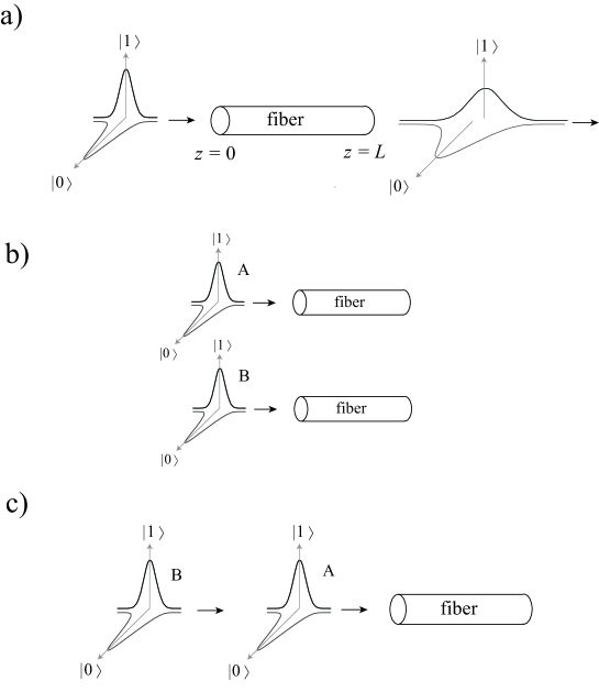
Figure 1: Single photon pulses passing through fibers of length $L$ along $z$ direction: a) A single-photon input pulse; b) two-photon entangled input pulses each passing through separate fibers; and c) two-photon entangled input pulses passing through a common fiber.

II A Model for Stochastic Polarization Mode Dispersion

In this section, we present basic equations for an optical pulse in optical fibers subjected to stochastic PMD PMDstat . In a single mode fiber, only two modes with orthogonal polarizations are supported. For an optical pulse propagating along $z$ in a linear and birefringent medium, fiber birefringence ${\bf b}(\omega,z)=b_{1}{\bf e}_{1}+b_{2}{\bf e}_{2}+b_{3}{\bf e}_{3}$, where ${\bf e}_{j}$ are unit vectors in the Stoke’s space, alters the polarization the field depending on its frequencies. The birefringence effect on the field modes, each of frequency $\omega$, can be derived directly from the wave equation, which gives

$$\frac{\partial^{2}}{\partial z^{2}}{\bf E}(\omega,z)+{\bf k}^{2}(\omega,z){\bf E}(\omega,z)=0.$$ (1)

Here ${\bf k}^{2}(\omega,z)\equiv\beta_{0}^{2}(\omega,z)+\beta_{0}(\omega,z){\bf b}(\omega,z)\cdot{\bm{\sigma}}$ is the propagation tensor, with $\beta_{0}(\omega,z)$ as the common propagation constant, and the vector ${\bm{\sigma}}$ is formed by the Pauli matrices given by ${\bm{\sigma}}=\hat{\sigma}_{1}{\bf e_{1}}+\hat{\sigma}_{2}{\bf e_{2}}+\hat{\sigma}_{3}{\bf e_{3}}$, with

$$\hat{\sigma}_{1}=\left(\begin{array}[]{cc}0&1\\ 1&0\end{array}\right),\ \ \ \hat{\sigma}_{2}=\left(\begin{array}[]{cc}0&-i\\ i&0\end{array}\right),\ \ \ \hat{\sigma}_{3}=\left(\begin{array}[]{cc}1&0\\ 0&-1\end{array}\right).$$ (2)

Extracting the fast oscillating common phase from the field, we define ${\bf E}(\omega,z)=E(\omega)\exp\left[-i\int_{0}^{z}\beta_{0}(\omega,z^{\prime})dz^{\prime}\right]{\bf A}(\omega,z)$ with $E(\omega)$ as the amplitude of the mode and ${\bf A}(\omega,z)$ as its frequency spectrum of the 2-dimensional Jones vector $\tilde{{\bf A}}(t,z)$ Agrawal

$${\bf A}(\omega,z)=\frac{1}{\sqrt{2\pi}}\int dt\tilde{{\bf A}}(t,z)\exp(i\omega t).$$ (3)

We adopt the adiabatic approximation, assuming that the birefringence vector ${\bf b}(\omega,z)$ and thus the polarization of the pulse varies slowly along $z$ PMD_review . As a consequence the term $\frac{\partial^{2}}{\partial z^{2}}{\bf A}(\omega,z)$ becomes negligible, and the effects of birefringence on the spectrum ${\bf A}(\omega,z)$, as the pulse passes through the fiber, can be described by the following first order differential equation PMD_review

$$i\frac{\partial}{\partial z}{\bf A}(\omega,z)=\frac{1}{2}\left[{\bf b}(\omega,z)\cdot{\bm{\sigma}}\right]{\bf A}(\omega,z).$$ (4)

Note that for non-dispersive channels, ${\bf b}(\omega,z)\cdot{\bm{\sigma}}$ gives eigenvalues $\pm\omega[n_{F}(z)-n_{S}(z)]/c$ determined by the refractive indices associated with the fast mode $n_{F}$ and slow mode $n_{S}$.

It is important to note that Eq. (4) is a kind of Schrödinger equation with the ‘Hamiltonian’ $\hat{h}=\frac{1}{2}\left[{\bf b}(\omega,z)\cdot{\bm{\sigma}}\right]$, in the form similar to that of a spin-half system interacting with a magnetic field. For deterministic evolution, we can express the output pulse with a unitary transformation,

$${\bf A}(\omega,L)=e^{-i{\hat{T}}\int^{L}_{0}\hat{{h}}dz}{\bf A}(\omega,0)$$ (5)

with ${\hat{T}}$ referring to a position ordered integration analogous to the time ordered integration in quantum theory. In terms of column vectors in Jones space, we have

$${\bf A}(\omega,0)\equiv\left(\begin{array}[]{cc}C_{1}^{{\rm in}}(\omega)\\ C_{0}^{{\rm in}}(\omega)\end{array}\right)\ \ \ \ \ \mbox{and}\ \ \ \ \ {\bf A}(\omega,L)\equiv\left(\begin{array}[]{cc}C_{1}^{{\rm out}}(\omega)\\ C_{0}^{{\rm out}}(\omega)\end{array}\right),$$ (6)

where $C_{j}^{{\rm in}}$ and $C_{j}^{{\rm out}}$ $(j=1,0)$ are polarization amplitudes for input and output fields obeying the normalization condition: $|C_{0}^{{\rm in}}|^{2}+|C_{1}^{{\rm in}}|^{2}=|C_{0}^{{\rm out}}|^{2}+|C_{1}^{{\rm out}}|^{2}=1$. For conceptual clarity, we will assume that the regions $z<0$ and $z>L$ are free of birefringence. In this way, ${\bf A}(\omega,z<0)={\bf A}(\omega,0)$ and ${\bf A}(\omega,z>L)={\bf A}(\omega,L)$.

The stochastic nature of our PMD model originates from the randomness of ${\bf b}(\omega,z)$. In this paper we adopt the assumption from Agrawal , that the randomness is due to the fluctuations of optical axis along the fiber. In addition, the frequency dependence of ${\bf b}(\omega,z)$ is determined by fiber material properties only and therefore should not change over different positions. In this way it is plausible to assume Agrawal :

$${\bf b}(\omega,z)=f(\omega){\bf b}(z)$$ (7)

where ${\bf b}(z)$ is stochastic, and the $f(\omega)$ is a deterministic function defined by the material and it can be expressed in terms of a Taylor series about the peak frequency $\omega_{0}$ of input pulses:

$$f(\omega)=\gamma\omega+\varsigma\omega(\omega-\omega_{0})+\cdots.$$ (8)

Note that in non-dispersive media, only the first term remains and most of our discussions below will be based on such an approximation. To specify the statistics of ${\bf b}(z)$, we assume that ${\bf b}(z)$ is a random process with zero mean, and it has the two-point correlation function Agrawal ; PMDstat :

$$\overline{{\bf b}(z_{1}){\bf b}(z_{2})}={\eta}^{2}\overleftrightarrow{{\bf I}}\delta(z_{2}-z_{1}).$$ (9)

Here the bar refers to the ensemble average, and ${\eta}$ characterizes the average strength of birefringence. We remark that the assumption of delta correlation function (9) is not a strict requirement. As long as the correlation length of ${\bf b}(z)$ is sufficiently short, in the sense that ${\bf A}(\omega,z)$ does not change significantly within the correlation length, then it is justified to employ the Markovian approximation in obtaining the master equation in later sections.

III General Description of Single and Two-photon states

Let us first examine a deterministic situation corresponding to a given realization of ${\bf b}(\omega,z)$. In the previous section, we have seen that if an incoming wave of frequency $\omega$ incident from the left with the polarization state $(C_{1}^{{\rm in}},C_{0}^{{\rm in}})$, then according to Eq. (5) and Eq. (6), there is an outgoing wave propagating to the right with the polarization state $(C_{1}^{{\rm out}},C_{0}^{{\rm out}})$. Since the system (or the wave equation) is linear, an incoming single-photon follows the same transformation rule to become an outgoing photon. Let $\phi(\omega)$ be the frequency envelope of the input single-photon wave packet, then the input and output state vectors, denoted by $|{\Psi_{{\rm in}}^{(1)}}\rangle$ and $|{\Psi_{{\rm out}}^{(1)}}\rangle$, take the form:

$$|{\Psi_{{\rm in}}^{(1)}}\rangle=\int{d\omega\phi(\omega)}\left|\omega\right\rangle\otimes\left[{C_{1}^{{\rm in}}(\omega)\left|1\right\rangle+C_{0}^{{\rm in}}(\omega)\left|0\right\rangle}\right]$$ (10)

$$|{\Psi_{\rm out}^{(1)}}\rangle=\int{d\omega\phi(\omega)}\left|\omega\right\rangle\otimes\left[{C_{1}^{{\rm out}}(\omega)\left|1\right\rangle+C_{0}^{{\rm out}}(\omega)\left|0\right\rangle}\right]$$ (11)

where $\left|\omega\right\rangle$ is the frequency basis vector defined in the birefringence free $[{\bf b}(\omega,z)=0]$ system, and $|1\rangle$ and $|0\rangle$ respectively correspond to horizontal and vertical polarization basis vectors. We point out that in writing Eq. (10) and (11), we have employed a rotating frame such that the phase factor $e^{-i\omega t}$ due to the free field evolution of $|\omega\rangle$ has been removed. This is equivalent to the representation in interaction picture. If Schrödinger picture is needed, we just need to replace $|\omega\rangle$ by $e^{-i\omega t_{{\rm in}}}|\omega\rangle$ in Eq. (10), and $|\omega\rangle$ by $e^{-i\omega t_{{\rm out}}}|\omega\rangle$ in Eq. (11), with $t_{{\rm in}}$ and $t_{{\rm out}}$ are instant of times defining the input and output states. Both $t_{{\rm in}}$ and $t_{{\rm out}}$ should be chosen in such a way that the input and output wave packets are far away from the birefringence interaction region.

It is important to note that if we treat the interaction length $L=z$ (Fig. 1) as a parameter, and let $|\Psi_{\rm out}^{(1)}(z)\rangle$ be the output state corresponding to a birefringence fiber of length $z$, then $|\Psi_{\rm out}^{(1)}(z)\rangle$ is governed by the Schrödinger-like equation according to Eq. (4), i.e.,

$$i\frac{\partial}{\partial z}{|{\Psi_{\rm out}^{(1)}(z)}\rangle}=\hat{\cal H}^{(1)}(z)|{\Psi_{\rm out}^{(1)}(z)}\rangle$$ (12)

where $z$ plays the role of time, and

$$\hat{\cal H}^{(1)}(z)=\int d\omega\left|\omega\right\rangle\left\langle\omega\right|\otimes\frac{1}{2}\left[{\bf b}(\omega,z)\cdot{\bm{\sigma}}\right]$$ (13)

plays the role of Hamiltonian.

In the case of two-photon states we will restrict our discussion to systems involving two distinct single-photon pulses, A and B, such that each pulse contains a single photon (Fig. 1). In other words, we can label the photons as two subsystems A and B. The distinguishability of the two photons can be achieved in two physical situations of interest here. The first situation is illustrated in Fig. 1b in which the two single-photon pulses individually propagate in two different optical fibers, and the second situation is when two spatially (or temporally) separated photons propagate in the same fiber (Fig. 1c). In both cases, we have the input-output state vectors:

$$|{\Psi_{\rm in}^{(2)}}\rangle=\int{\int{d\omega_{A}d\omega_{B}\phi(\omega_{A},\omega_{B})}\left|{\omega_{A},\omega_{B}}\right\rangle\otimes\sum\limits_{s_{A},s_{B}=0,1}{C_{s_{A}s_{B}}^{{\rm in}}}}(\omega_{A},\omega_{B})\left|{s_{A},s_{B}}\right\rangle$$ (14)

$$|{\Psi_{\rm out}^{(2)}}\rangle=\int{\int{d\omega_{A}d\omega_{B}\phi(\omega_{A},\omega_{B})}\left|{\omega_{A},\omega_{B}}\right\rangle\otimes\sum\limits_{s_{A},s_{B}=0,1}{C_{s_{A}s_{B}}^{{\rm out}}}}(\omega_{A},\omega_{B})\left|{s_{A},s_{B}}\right\rangle$$ (15)

with $\phi(\omega_{A},\omega_{B})$ being the normalized frequency envelope of the input 2-photon wave packet, i.e., $\int\int d\omega_{A}d\omega_{B}|\phi(\omega_{A},\omega_{B})|^{2}=1$, and the $C_{s_{A}s_{B}}^{{\rm in}}(\omega)$ and $C_{s_{A}s_{B}}^{{\rm out}}$ describe the joint polarization amplitudes for input and output states at the corresponding frequencies. We remark that input states with non-factorizable $\phi(\omega_{A},\omega_{B})$ correspond to frequency entangled states, and similarly, non-separable $C_{s_{A}s_{B}}^{{\rm in}}$ means polarization entanglement.

The fact that the two distinguishable single-photons do not interact allows us to treat their evolution by the transformation rule as in the case of single photon. Similar to Eq.(12), we can treat the interaction length $L=z$ as a parameter and obtain the Schrödinger equation,

$$i\frac{\partial}{\partial z}{|{\Psi_{\rm out}^{(2)}(z)}\rangle}=\hat{\cal H}^{(2)}(z)|{\Psi_{\rm out}^{(2)}(z)}\rangle$$ (16)

with

$$\hat{\cal H}^{(2)}(z)=\frac{1}{2}\int d\omega\left[{\bf b}_{1}(\omega,z)\cdot{\bm{\sigma}^{(A)}}\otimes\left|\omega\right\rangle_{A}\left\langle\omega\right|+{\bf b}_{2}(\omega,z)\cdot{\bm{\sigma}^{(B)}}\otimes\left|\omega\right\rangle_{B}\left\langle\omega\right|\right]$$ (17)

for the case of separate fiber (Fig. 1b), and ${\bf b}_{1}(\omega,z)$ and ${\bf b}_{2}(\omega,z)$ are birefringence vectors of the two fibers. The ${\bm{\sigma}^{(A)}}$ and ${\bm{\sigma}^{(B)}}$ are Pauli vectors for photons A and B.

In the case of common fiber (Fig. 1c), we have

$$\hat{\cal H}^{(2)}(z)=\frac{1}{2}\int d\omega{\bf b}(\omega,z)\cdot\left[{\bm{\sigma}^{(A)}}\otimes\left|\omega\right\rangle_{A}\left\langle\omega\right|+{\bm{\sigma}^{(B)}}\otimes\left|\omega\right\rangle_{B}\left\langle\omega\right|\right].$$ (18)

which indicates that both photons experience the same birefringence interaction. Note that the pure state vectors discussed above can be considered as quantum trajectories, corresponding to a single realization of a birefringence vector. To address the stochastic problem, we will need to to perform averaging via the density matrices. In later sections, theoretical analysis of the density matrices will be carried out according to the master equations for each of the cases in Fig. 1.

IV Decoherence of a single-photon state

Let us first discuss the master equation describing a single-photon state passing through the fiber. From Eq. (12), the density operator $\hat{\rho}^{(1)}_{s}(z)$ of the state obeys the equation

$$i\frac{\partial\hat{\rho}^{(1)}_{s}(z)}{\partial z}={[\hat{{\cal H}}^{(1)}(z),\hat{\rho}^{(1)}_{s}(z)]},$$ (19)

where the subscript $s$ stands for a given realization of birefringence defining $\hat{{\cal H}}^{(1)}(z)$, i.e., before taking the ensemble average. We follow the standard strategy to obtain the master equation bloch ,

$$\frac{\partial}{\partial z}\hat{\rho}^{(1)}= \frac{\eta^{2}}{4}\sum_{i=1}^{3}\left[2\hat{\Gamma}_{i}\hat{\rho}^{(1)}\hat{\Gamma}_{i}-\hat{\Gamma}_{i}\hat{\Gamma}_{i}\hat{\rho}^{(1)}-\hat{\rho}^{(1)}\hat{\Gamma}_{i}\hat{\Gamma}_{i}\right],$$ (20)

where we have used $\hat{\rho}^{(1)}\equiv\overline{\hat{\rho}^{(1)}_{s}}$ in order to simplify the notation, and $\hat{\Gamma}_{i}\equiv\int d\omega f(\omega)\left|\omega\right\rangle\left\langle\omega\right|\otimes\hat{\sigma_{i}}$ is defined. For later purposes the single-photon density matrix can be expressed explicitly by,

$$\hat{\rho}^{(1)}(z)={\int{\int{d\omega d\omega^{\prime}\sum\limits_{s,s^{\prime}=0,1}\rho_{ss^{\prime}}\left({\omega,\omega^{\prime};z}\right)}}}\left|{\omega,s}\right\rangle\left\langle{\omega^{\prime},s^{\prime}}\right|$$ (21)

where $\rho_{ss^{\prime}}\left({\omega,\omega^{\prime};L}\right)$ are matrix elements.

We point out that the derivation of the master equation Eq. (20) is based on the Bloch-Redfield-Wangsness approach known in nuclear magnetic resonance literature bloch . Alternatively, the same master equation can be derived by treating the fiber medium as a bath with many degrees of freedom gardiner ; limitations . The former approach, which we adopt here, can be understood more transparently by considering the fiber as composed of concatenating uncorrelated short sections of length $\Delta z$, and $\Delta z$ is set to be long compared with the coherence length of ${\bf b}(z)$, but is small so that the change of state can be approximated by keeping the Dyson series up to the second order in $\hat{{\cal H}}^{(1)}$. Then by Markovian approximation Eq. (9), the master equation (20) in fact corresponds to the ‘coarse rate of variation’ $\Delta\hat{\rho}^{(1)}_{s}/\Delta z$ upon ensemble average.

Now, we consider a general single-photon pulse which is initially polarized along $\left|1\right\rangle$,

$$\left|\Psi_{in}\right\rangle=\left|1\right\rangle\otimes\int d\omega\phi(\omega)\left|\omega\right\rangle.$$ (22)

We remark that the result is the same for arbitrary polarization direction due to the symmetry caused by the randomizing effect of the birefringence fluctuations, and hence we set it to $\left|1\right\rangle$ for convenience. The input pulse envelope is set as a Gaussian wave packet

$$\phi(\omega)=\left(\frac{2}{\kappa^{2}\pi}\right)^{1/4}\exp\left[\frac{-(\omega-\omega_{0})^{2}}{\kappa^{2}}\right],$$ (23)

where $\kappa$ indicates the width of the Gaussian envelope and the peak frequency $\omega_{0}$ is in the optical range. With the input condition $\hat{\rho}_{in}=\left|1\right\rangle\left\langle 1\right|\otimes\int\int d\omega d\omega^{\prime}\phi(\omega)\phi^{*}(\omega^{\prime})\left|\omega\right\rangle\left\langle\omega^{\prime}\right|$, we solve the output state governed by the master equation Eq. (20), and the details are presented in Appendix (A). The solution for the density matrix is given by,

$$\rho_{11}(\omega,\omega^{\prime};L) = \frac{1}{2}\phi(\omega)\phi^{*}(\omega^{\prime})\left(e^{-\lambda_{1}L}+e^{-\lambda_{2}L}\right)$$

$$\rho_{00}(\omega,\omega^{\prime};L) = \frac{1}{2}\phi(\omega)\phi^{*}(\omega^{\prime})\left(e^{-\lambda_{1}L}-e^{-\lambda_{2}L}\right),$$ (24)

where the values of $\lambda_{i}\geq 0$ at given $\omega$, $\omega^{\prime}$ are

$$\lambda_{1}(\omega,\omega^{\prime}) = \frac{3\eta^{2}}{4}[f(\omega)-f(\omega^{\prime})]^{2}$$

$$\lambda_{2}(\omega,\omega^{\prime}) = \frac{\eta^{2}}{4}[3f(\omega)^{2}+3f(\omega^{\prime})^{2}+2f(\omega)f(\omega^{\prime})],$$ (25)

It is interesting to note that $\lambda_{1}$ is a difference of the frequency profiles and $\lambda_{2}$ is a sum, giving $\lambda_{1}\ll\lambda_{2}$ in the optical region. The off diagonal elements are $\rho_{10}(\omega,\omega^{\prime};L)=\rho_{01}(\omega,\omega^{\prime};L)=0$. Having solved the matrix elements, the output density matrix $\hat{\rho}^{(1)}(L)$ can therefore be obtained according to Eq. (21). It can be observed that in the long length limit $L\rightarrow\infty$, a complete depolarization occurs, since only diagonal elements $\rho_{11}(\omega,\omega;L)=\rho_{00}(\omega,\omega;L)=\frac{1}{2}|\phi(\omega)|^{2}$ remain.

IV.1 Pulse spreading

Let us introduce the quantized field operator,

$$\hat{{\cal E}}(z,t)=\int d\omega\ e^{i\omega(z-ct)/c}\hat{a}_{\omega}+h.c.$$ (26)

where $\hat{a}_{\omega}$ is the corresponding annihilation operator. To visualize the change of output pulse shape due to PMD, we examine the intensity operator $\hat{I}\equiv\hat{\cal E}^{\dagger}\hat{\cal E}$ by evaluating its expectation value with respect to the output pulse. The calculation is quite tedious, and we present the results only. For linear non-dispersive fibers $f(\omega)=\gamma\omega$, we find that the spatial dependence of the averaged output intensity associated with the two polarization states are given by

$$\langle\hat{I}(\tau)\rangle_{1} = \sqrt{\frac{\pi}{2}}\left\{\frac{e^{-\frac{\kappa^{2}\tau^{2}}{2[1+6L/(L_{c}\nu^{2})]}}}{\sqrt{1+6L/(L_{c}\nu^{2})}}+\frac{e^{-\frac{\kappa^{2}\tau^{2}}{2[1+2L/(L_{c}\nu^{2})]}-\frac{8L/L_{c}}{1+4L/(L_{c}\nu^{2})}}}{\sqrt{[1+2L/(L_{c}\nu^{2})][1+4L/(L_{c}\nu^{2})]}}\right\}$$

$$\langle\hat{I}(\tau)\rangle_{0} = \sqrt{\frac{\pi}{2}}\left\{\frac{e^{-\frac{\kappa^{2}\tau^{2}}{2[1+6L/(L_{c}\nu^{2})]}}}{\sqrt{1+6L/(L_{c}\nu^{2})}}-\frac{e^{-\frac{\kappa^{2}\tau^{2}}{2[1+2L/(L_{c}\nu^{2})]}-\frac{8L/L_{c}}{1+4L/(L_{c}\nu^{2})}}}{\sqrt{[1+2L/(L_{c}\nu^{2})][1+4L/(L_{c}\nu^{2})]}}\right\}$$ (27)

where $\tau=z/c-t$, with $t$ being a sufficiently long time so that the entire pulse has exited from the birefringence fiber of length $L$. In addition we have defined the characteristic decoherence length

$$L_{c}\equiv\left(\frac{\eta^{2}}{4}\gamma^{2}\omega_{0}^{2}\right)^{-1},$$ (28)

and the dimensionless ratio $\nu\equiv\omega_{0}/\kappa$.

In the narrow bandwidth case where $\nu\gg 1$, the second term in Eq. (IV.1) decay approximately exponentially with the decay length $L_{c}/8$. Such a decaying length scale is much shorter than that in the first term. Therefore as $L\gg L_{c}$ increases, only the first term remains, equalizing both elements and hence showing depolarization. It can be seen that the width of the output pulse is approximately $c\sqrt{2[1+6L/(L_{c}\nu^{2})]}/\kappa$, which has a $\sqrt{L}$ dependence when $L\gg L_{c}\nu^{2}$ is sufficiently large. Such a $\sqrt{L}$ dependence were also reported in general classical consideration Gisin1995 . The pulse width at the output is greater than that of input, thus sets a lower bound to the distance between input pulses in order to allow the output pulses to be non-overlapping, or distinguishable.

IV.2 Purity functions

Next, we investigate the decoherence of the single-photon pulse through its purity defined as $\mu\equiv{\rm Tr}(\hat{\rho}^{2})\leq 1$. Purity is closely related to the reciprocal number of effective modes required to contain the whole state, hence the equality sign holds only when the state is pure, i.e. can be completely represented by one mode of the basis. We calculate the frequency purity, the polarization purity and the overall purity.

To obtain the frequency purity, we trace the polarization freedom of $\hat{\rho}^{(1)}(L)$ and consider only the frequency DOF. From Eq. (21) and Eq. (IV), noting that

$${\rm Tr}_{s}(\hat{\rho}^{(1)}(L))=\int\int d\omega d\omega^{\prime}\phi(\omega)\phi^{*}(\omega^{\prime})e^{-\lambda_{1}L}\left|\omega\right\rangle\left\langle\omega^{\prime}\right|,$$ (29)

the frequency purity is given by,

$$\mu_{\omega}(L) = {\rm Tr}\left\{[{\rm Tr}_{s}(\hat{\rho}^{(1)}(L))]^{2}\right\}=\frac{1}{\sqrt{1+6L/(L_{c}\nu^{2})}},$$ (30)

which decays algebraically with $L$. Note that $\mu_{\omega}(L)$ depends on a decay length scale $\nu^{2}L_{c}$, meaning that $\mu_{\omega}(L)$ has a slower decay rate for a greater $\nu$, i.e., narrower spectrum. A remark is that the effective number of frequency modes (as measured by $\mu_{\omega}^{-1}$) required to represent the state increases from $1$ to infinity as $L$ increases. In fact, $\mu_{\omega}^{-1}$ shares a similar functional form with the output pulse width described in the previous section. This suggests that the pulse widening can be a measure of PMD decoherence of frequency variables for Gaussian initial states.

Next we find the polarization purity of $\hat{\rho}^{(1)}(L)$ after tracing the frequency freedom from $\hat{\rho}^{(1)}(L)$. Noting that

$${\rm Tr}_{\omega}(\hat{\rho}^{(1)}(L)) = {\int{d\omega[\rho_{11}\left({\omega,\omega;L}\right)\left|{1}\right\rangle\left\langle{1}\right|+\rho_{00}\left({\omega,\omega;L}\right)}}\left|{0}\right\rangle\left\langle{0}\right|],$$ (31)

the polarization purity $\mu_{s}(L)$ is therefore

$$\mu_{s}(L) = {\rm Tr}\left\{[{\rm Tr}_{\omega}(\hat{\rho}^{(1)}(L))]^{2}\right\}$$ (32)

$$= \left[\int d\omega\rho_{11}\left(\omega,\omega;L\right)\right]^{2}+\left[\int d\omega\rho_{00}\left(\omega,\omega;L\right)\right]^{2}$$

$$= \frac{1}{2}\left[1+\frac{1}{1+4L/(L_{c}\nu^{2})}e^{-\frac{16L/L_{c}}{1+4L/(L_{c}\nu^{2})}}\right],$$

decreasing from $1$ to the minimum value $1/2$, meaning that the state is more spread out in the 2-dimensional Jones space to the fully mixed situation as fiber length increases. Note that the decay length scale for $\mu_{s}(L)$ is $L_{c}/16$ in the narrow bandwidth case with $\nu\gg 1$, which is shorter than that for $\mu_{\omega}(L)$. In addition, appearance of the exponential factor in Eq. (32) indicates a faster decay rate than that of $\mu_{\omega}(L)$.

The total purity is also found by

$$\mu_{total}(L) = {\rm Tr}\left\{[\hat{\rho}^{(1)}(L)]^{2}\right\}$$ (33)

$$= \frac{1}{2}\left\{\frac{1}{\sqrt{1+6L/(L_{c}\nu^{2})}}+\frac{e^{-\frac{16L/L_{c}}{1+4L/(L_{c}\nu^{2})}}}{\sqrt{[1+2L/(L_{c}\nu^{2})][1+4L/(L_{c}\nu^{2})]}}\right\},$$

again having a slower rate of decay for a greater $\nu$, and obeying $\mu_{\omega}(L)\cdot\mu_{s}(L)\leq\mu_{total}(L)$. We conclude that decoherence for single-photon state in Eq. (22) is complete only upon $L\rightarrow\infty$.

V Disentanglement of two-photon states in separate fibers

In this section we study the disentanglement of an entangled two-photon state propagating along separate fibers, each with random birefringence ${\bf b}_{i}(z)$ for $(i=1,2)$. We assume that they are made from the same material, hence obeying $\left\langle{\bf b}_{i}(z_{1}){\bf b}_{j}(z_{2})\right\rangle=\eta^{2}\overleftrightarrow{{\bf I}}\delta_{ij}\delta(z_{2}-z_{1})$. The ‘Hamiltonian’ in this case is given by Eq. (17). With similar assumptions as in the single-photon situation, we obtain the master equation governing the ensemble averaged density matrix $\hat{\rho}^{(2)}\equiv\overline{\hat{\rho}^{(2)}_{s}}$

$$\frac{\partial}{\partial z}\hat{\rho}^{(2)}= \frac{\eta^{2}}{4}\sum_{j=A,B}\sum_{i=1}^{3}\left[2\hat{\Gamma}^{(j)}_{i}\hat{\rho}^{(2)}\hat{\Gamma}^{(j)}_{i}-\hat{\Gamma}^{(j)}_{i}\hat{\Gamma}^{(j)}_{i}\hat{\rho}^{(2)}-\hat{\rho}^{(2)}\hat{\Gamma}^{(j)}_{i}\hat{\Gamma}^{(j)}_{i}\right],$$ (34)

where $\hat{\Gamma}^{(j)}_{i}\equiv\int d\omega f(\omega)\left|\omega\right\rangle_{j}\left\langle\omega\right|\otimes\hat{\sigma}_{i}^{(j)}$ for the two photons $j=A,B$. It can be noted that the master equation consists of two decoupled parts, each for an individual fiber. As in the previous section, it will be convenient to write the two-photon density matrix explicitly

$$\hat{\rho}^{(2)}(z)={\int{\int{\int{\int{}}d\omega_{A}d\omega_{B}d\omega_{A}^{\prime}d\omega_{B}^{\prime}\sum\limits_{s_{A}s_{B}s_{A}^{\prime}s_{B}^{\prime}=0,1}\rho_{s_{A}s_{B}s_{A}^{\prime}s_{B}^{\prime}}\left({\omega_{A},\omega_{B},\omega_{A}^{\prime},\omega_{B}^{\prime};z}\right)}}}$$

$$\times\left|{\omega_{A},\omega_{B}}\right\rangle\left\langle{\omega_{A}^{\prime},\omega_{B}^{\prime}}\right|\otimes\left|{s_{A},s_{B}}\right\rangle\left\langle{s_{A}^{\prime},s_{B}^{\prime}}\right|.$$ (35)

with the matrix elements $\rho_{s_{A}s_{B}s_{A}^{\prime}s_{B}^{\prime}}\left({\omega_{A},\omega_{B},\omega_{A}^{\prime},\omega_{B}^{\prime};z}\right)$.

In this section we investigate an initially hyperentangled state hyperent , a polarization Bell state with frequency entanglement:

$$|{\Psi_{\rm in}^{(2)}}\rangle=\int\int\phi(\omega_{A},\omega_{B})d\omega_{A}d\omega_{B}\left|\omega_{A},\omega_{B}\right\rangle\otimes\left|\psi_{\rm Bell}\right\rangle,$$ (36)

where the frequency envelope is assumed to be a double Gaussian, with a peak frequency $\omega_{0}$, as follows:

$$\phi(\omega_{A},\omega_{B})=\sqrt{\frac{4\alpha\beta}{\pi}}\exp[-\alpha^{2}(\omega_{A}-\omega_{B})^{2}-\beta^{2}(\omega_{A}+\omega_{B}-2\omega_{0})^{2}],$$ (37)

where the width $\alpha>\beta$ corresponds to a more frequency correlated state and $\beta>\alpha$ indicates a more frequency anticorrelated state. We consider an input singlet pulse $\left|\psi_{\rm Bell}\right\rangle=\frac{1}{\sqrt{2}}(|10\rangle-|01\rangle)$. The evolution of the four Bell states, including the singlet state and the triplet states, follow same calculation steps and thus only the singlet state evolution is discussed in detail, presented in Appendix (B).

Following the master equation Eq. (34), the evolution of the only non-zero density matrix elements at $\omega_{A},\omega_{B},\omega_{A}^{\prime},\omega_{B}^{\prime}$ can be found as

$$\rho_{1111} = \rho_{0000}=\frac{1}{4}\phi(\omega_{A},\omega_{B})\phi^{*}(\omega_{A}^{\prime},\omega_{B}^{\prime})\left(e^{-\zeta_{1}L}-e^{-\zeta_{4}L}\right)$$

$$\rho_{1010} = \rho_{0101}=\frac{1}{4}\phi(\omega_{A},\omega_{B})\phi^{*}(\omega_{A}^{\prime},\omega_{B}^{\prime})\left(e^{-\zeta_{1}L}+e^{-\zeta_{4}L}\right)$$

$$\rho_{1001} = \rho_{0110}=-\frac{1}{2}\phi(\omega_{A},\omega_{B})\phi^{*}(\omega_{A}^{\prime},\omega_{B}^{\prime})e^{-\zeta_{4}L},$$ (38)

where the values of $\zeta_{i}$ at given $\omega_{A}$, $\omega_{B}$, $\omega_{A}^{\prime}$ and $\omega_{B}^{\prime}$ are shown in Eq. (B). We can see that $\zeta_{1}\ll\zeta_{4}$ in the optical region. We remark that the Bell states have zero projection to the spaces characterized by $\zeta_{2}$ and $\zeta_{3}$ and therefore $\zeta_{2}$ and $\zeta_{3}$ do not contribute to the state evolution, which is shown in Appendix (B). In particular, $\zeta_{1}=0$ only for the diagonal elements, and thus the steady state is a completely depolarized one, with $\rho_{1111}=\rho_{1010}=\rho_{0101}=\rho_{0000}=\frac{1}{4}|\phi(\omega_{A},\omega_{B})|^{2}$.

V.1 Characterization of entanglement in terms of negativity

According to Peres and Horodecki’s PPT (positive partial transposition) criterion PPTperes ; PPThoro1 ; PPThoro , if the partial transposition of a bipartite density matrix (denoted by $\rho^{T_{A}}$) has one or more negative eigenvalues, then the state is an entangled state. The negativeness of $\rho^{T_{A}}$ turns out to be a necessary and sufficient condition of mixed state entanglement for two-qubit states and bipartite Gaussian states. To quantify how much entanglement survives by PMD decoherence in polarization and frequency variables, we calculate the negativity of the corresponding DOFs.

The negativity ${\cal N}$ of the state $\hat{\rho}$ is defined by monotone

$${\cal N}=\frac{||\hat{\rho}^{T_{A}}||-1}{2}$$ (39)

which is an entanglement monotone under local operation and classical communication monotone . Specifically, the polarization negativity is found by first tracing the frequency variables and taking the trace norm of the partial transposition ($s_{A}\leftrightarrow s_{A}^{\prime}$), i.e.

$${\cal N}_{s}=\frac{||\{{\rm Tr}_{\omega_{A},\omega_{B}}[\hat{\rho}^{(2)}(L)]\}^{T_{A}}||-1}{2}.$$ (40)

Similarly, the frequency negativity is obtained by finding the trace norm of the partially transposed density matrix with the polarization variables traced, i.e.,

$${\cal N}_{\omega}=\frac{||\{{\rm Tr}_{s_{A},s_{B}}[\hat{\rho}^{(2)}(L)]\}^{T_{A}}||-1}{2}.$$ (41)

Equivalently, negativities can be obtained by summing the absolute value of negative eigenvalues of the partially transposed matrices negsum , which we adopt in the following sections.

V.2 Polarization disentanglement

Now we discuss polarization disentanglement of the two-photon output state by finding the negativity ${\cal N}_{s}$ of the state. We first obtain

$$\{{\rm Tr}_{\omega_{A},\omega_{B}}[\hat{\rho}^{(2)}(L)]\}^{T_{A}} = \int\int d\omega_{A}d\omega_{B}\left(\begin{array}[]{cccc}\rho_{1111}&0&0&0\\ 0&\rho_{1010}&\rho_{1001}&0\\ 0&\rho_{0110}&\rho_{0101}&0\\ 0&0&0&\rho_{0000}\end{array}\right)^{T_{A}}$$ (46)

$$= \left(\begin{array}[]{cccc}\frac{1}{4}(1-\chi)&0&0&-\frac{1}{2}\chi\\ 0&\frac{1}{4}(1+\chi)&0&0\\ 0&0&\frac{1}{4}(1+\chi)&0\\ -\frac{1}{2}\chi&0&0&\frac{1}{4}(1-\chi)\end{array}\right),$$ (51)

where by assuming $f(\omega)=\gamma\omega$,

$$\chi=\exp\left.\left[\frac{-16L/L_{c}}{1+(2L/\beta^{2}\omega_{0}^{2}L_{c})}\right]\right/\sqrt{\left(1+\frac{2L}{\alpha^{2}\omega_{0}^{2}L_{c}}\right)\left(1+\frac{2L}{\beta^{2}\omega_{0}^{2}L_{c}}\right)}.$$ (52)

The polarization negativity ${\cal N}_{s}$ can thus be found as

$${\cal N}_{s}=\frac{3}{4}\chi-\frac{1}{4}.$$ (53)

Note that Eq. (53) is applicable to all four Bell states since we have the freedom to redefine the polarization bases and phases in the second fiber due to the symmetry caused by the stochastic birefringence fluctuations. We also remark that ${\cal N}_{s}$ has a decay length scale $L_{c}/16$, and we note that the same decay length scale exists for polarization purity in the single photon case. In addition, we observe that finite length disentanglement is possible when $\chi\leq 1/3$, which can be solved numerically. As the exponential factor of $\chi$ is depending on the value of $\beta$, we fix $\alpha$ and plot the trend of polarization negativity with varying $\beta\omega_{0}$ in Fig. 2. We see that in general the critical disentanglement length increases and peaks at some value of $\beta\omega_{0}$, then level off to some finite value as $\beta\omega_{0}$ tends to infinity.

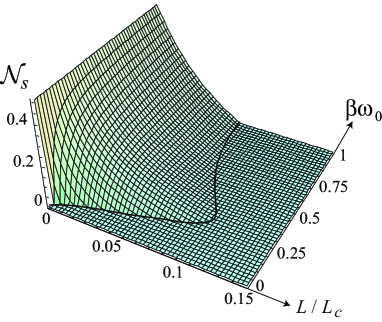
Figure 2: The polarization negativity for the two-photon separate fiber case for $\alpha\omega_{0}=1000$ with varying $\beta$ and $L$. The black solid curve indicates the critical disentanglement length.

V.3 Frequency disentanglement

To calculate the frequency negativity, we trace the polarization variables as follows:

$${\rm Tr}_{s_{A},s_{B}}[\hat{\rho}^{(2)}(L)] = \int\int\int\int d\omega_{A}d\omega_{B}d\omega_{A}^{\prime}d\omega_{B}^{\prime}$$ (54)

$$\phi(\omega_{A},\omega_{B})\phi^{*}(\omega_{A}^{\prime},\omega_{B}^{\prime})e^{-\zeta_{1}L}|\omega_{A},\omega_{B}\rangle\langle\omega_{A}^{\prime},\omega_{B}^{\prime}|$$

It is insightful to note that this equation holds not only for Bell states, but for any general initial polarization states having the form of Eq. (36) two_sep_freqneg . An important consequence is that frequency entanglement in separate fibers is independent to initial polarization status. This result is in contrast to the polarization negativity we presented previously, which is dependent on the initial frequency envelope shape.

The partial transposition of the frequency density matrix can be found by $\rho^{T_{A}}(\omega_{A},\omega_{B},\omega_{A}^{\prime},\omega_{B}^{\prime})=\langle\omega_{A}^{\prime},\omega_{B}|{\rm Tr}_{s_{A},s_{B}}[\hat{\rho}^{(2)}(L)]|\omega_{A},\omega_{B}^{\prime}\rangle$. For linear non-dispersive medium $f(\omega)=\gamma\omega$, the frequency density matrix remains Gaussian. This allows us to determine its negativity can be analytically from the general formula for Gaussian states in PoonNeg ,

$${\cal N}_{\omega}=\left\{\begin{array}[]{cc}\frac{1}{2}\left(\sqrt{\frac{\alpha^{2}\omega_{0}^{2}L_{c}}{\beta^{2}\omega_{0}^{2}L_{c}+3L}}-1\right)\ \ \ \ \mbox{for}\ \ \ \ \alpha^{2}\omega_{0}^{2}L_{c}>\beta^{2}\omega_{0}^{2}L_{c}+3L\\ \frac{1}{2}\left(\sqrt{\frac{\beta^{2}\omega_{0}^{2}L_{c}}{\alpha^{2}\omega_{0}^{2}L_{c}+3L}}-1\right)\ \ \ \ \mbox{for}\ \ \ \ \beta^{2}\omega_{0}^{2}L_{c}>\alpha^{2}\omega_{0}^{2}L_{c}+3L\end{array}\right..$$ (57)

It is interesting to see that finite length frequency disentanglement occurs when

$$L\geq\frac{\omega_{0}^{2}}{3}|\alpha^{2}-\beta^{2}|L_{c},$$ (58)

which is universal to any initial polarization state. The expression signifies that the system is ‘less robust’, i.e. having the critical length of disentanglement tends to zero, if the initial frequency envelope has $\alpha\approx\beta$. Note that the polarization entanglement mainly depends on the value of $\beta$, while the frequency entanglement increases with the difference between $\alpha^{2}$ and $\beta^{2}$.

VI Disentanglement of two-photon states in a common fiber

Next, we examine the decoherence problem for two photons propagating in the same fiber of length $L$. Physically, we can distinguish the two photons by spatially separate them by a small distance, so small that the two photons still experience the same stochastic interactions with the fiber birefringence, yet far apart enough to be distinguishable, depending on the width of the output pulse which is discussed quantitatively in the single-photon section. The ‘Hamiltonian’ in this case is given by Eq.(18). The master equation is as follows:

$$\frac{\partial}{\partial z}\hat{\rho}^{(2)}= \frac{\eta^{2}}{4}\sum_{i=1}^{3}\left[2\hat{\Lambda}_{i}\hat{\rho}^{(2)}\hat{\Lambda}_{i}-\hat{\Lambda}_{i}\hat{\Lambda}_{i}\hat{\rho}^{(2)}-\hat{\rho}^{(2)}\hat{\Lambda}_{i}\hat{\Lambda}_{i}\right],$$ (59)

where

$$\hat{\Lambda}_{i} \equiv \int\int d\omega_{A}d\omega_{B}[f(\omega_{A})\hat{\sigma}^{(A)}_{i}+f(\omega_{B})\hat{\sigma}^{(B)}_{i}]\otimes\left|\omega_{A},\omega_{B}\right\rangle\left\langle\omega_{A},\omega_{B}\right|.$$ (60)

We remark that the form of this equation is similar to the single photon master equation Eq. (20), but with the collective operator $\hat{\Lambda}_{i}$.

It is known that two photons of same frequencies in singlet polarization states lie in DFS, and their resistance to decoherence has been verified experimentally singletexpt . The reason behind the decoherence free effect is that they are eigenstates of $\hat{{\cal H}}^{(2)}$ with an zero eigenvalue, meaning that these states do not evolve as they propagate. The key is the identical coupling with the environment for both of the photons limitations . In practice, however, photons generally have fluctuations in frequencies variables. In the case of down conversion systems, the two photons are in fact anti-correlated due to energy conservation. It is thus of interest to examine the robustness of entanglement for singlet polarization states with a general Gaussian frequency envelope $\phi(\omega_{A},\omega_{B})$,

$$|{\Psi_{\rm in}^{(2)}}\rangle=\int\int\phi(\omega_{A},\omega_{B})e^{-i\omega_{A}z_{0}/c}d\omega_{A}d\omega_{B}\left|\omega_{A},\omega_{B}\right\rangle\otimes\left[\frac{1}{\sqrt{2}}(\left|10\right\rangle-\left|01\right\rangle)\right]$$ (61)

where $\phi(\omega_{A},\omega_{B})$ is a double Gaussian given in Eq. (37), and the phase factor $e^{-i\omega_{A}z_{0}/c}$ is added in order to displace the peak position of the photon wave packet A by a distance $z_{0}$ relative to B. The choice of separation $z_{0}$ should be large compared with the width of the wave packets so that the two photons can be treated as distinct subsystems, but small enough so that both photons would experience the same stochastic birefringence. Note that the displacement of photon A is simply achieved by a local unitary transformation operator: $\exp(-iz_{0}\int\frac{\omega}{c}|\omega\rangle_{A}\langle\omega|d\omega)$, and it commutes with $\hat{\cal H}^{(2)}$ in Eq. (18). Therefore the phase factor do not affect the entanglement. For convenience, we will simply absorb the phase factor into the definition of $|\omega\rangle_{A}$ in the later calculations.

Following the master equation in Eq. (59), the singlet state evolution at $\omega_{A},\omega_{B},\omega_{A}^{\prime},\omega_{B}^{\prime}$ are found by the steps in Appendix (C), and are presented as follows.

$$\left(\begin{array}[]{cccc}\rho_{1111}&\rho_{1110}&\rho_{1101}&\rho_{1100}\\ \rho_{1011}&\rho_{1010}&\rho_{1001}&\rho_{1000}\\ \rho_{0111}&\rho_{0110}&\rho_{0101}&\rho_{0100}\\ \rho_{0011}&\rho_{0010}&\rho_{0001}&\rho_{0000}\end{array}\right)_{L} = \left(\begin{array}[]{cccc}\frac{1}{\sqrt{3}}v_{2}&0&0&0\\ 0&\frac{1}{2}v_{1}+\frac{1}{2\sqrt{3}}v_{2}&-\frac{1}{2}v_{1}+\frac{1}{2\sqrt{3}}v_{2}&0\\ 0&-\frac{1}{2}v_{1}+\frac{1}{2\sqrt{3}}v_{2}&\frac{1}{2}v_{1}+\frac{1}{2\sqrt{3}}v_{2}&0\\ 0&0&0&\frac{1}{\sqrt{3}}v_{2}\end{array}\right),$$ (70)

where

$$v_{1} = \frac{1}{2}\phi(\omega_{A},\omega_{B})\phi^{*}(\omega_{A}^{\prime},\omega_{B}^{\prime})\left\{\left[\frac{-V^{(1)}_{11}+V^{(1)}_{22}}{\sqrt{\left(V^{(1)}_{11}-V^{(1)}_{22}\right)^{2}+4{V^{(1)}_{12}}^{2}}}+1\right]e^{-\xi_{1}L}\right.$$

$$\ \ \ \ \ \ \ \ \ \ \ \ \ \ \ \ \ \ \ \ \ \ \ \ \ \ \ \ \ \left.+\left[\frac{V^{(1)}_{11}-V^{(1)}_{22}}{\sqrt{\left(V^{(1)}_{11}-V^{(1)}_{22}\right)^{2}+4{V^{(1)}_{12}}^{2}}}+1\right]e^{-\xi_{2}L}\right\}$$

$$v_{2} = \frac{V^{(1)}_{12}\phi(\omega_{A},\omega_{B})\phi^{*}(\omega_{A}^{\prime},\omega_{B}^{\prime})}{\sqrt{\left(V^{(1)}_{11}-V^{(1)}_{22}\right)^{2}+4{V^{(1)}_{12}}^{2}}}\left(-e^{-\xi_{1}L}+e^{-\xi_{2}L}\right)$$ (71)

having $\xi_{i}\geq 0$ denoted in Eq. (C), with $\xi_{1}\gg\xi_{2}$ in the optical region.

An important situation to notice is when $\xi_{2}=0$, where no decay occurs and the matrix elements can survive to infinite fiber length. It can be noted that $\xi_{2}=0$ only for three cases, when $\omega_{A}=\omega_{A}^{\prime}$ and $\omega_{B}=\omega_{B}^{\prime}$, $\omega_{A}=\omega_{B}$ and $\omega_{A}^{\prime}=\omega_{B}^{\prime}$, or $\omega_{A}=\omega_{B}^{\prime}$ and $\omega_{A}^{\prime}=\omega_{B}$ (Appendix C). Thus we obtain the output state in the $L\rightarrow\infty$ limit, with the only nonzero terms as follows:

$$\omega_{A}=\omega_{A}^{\prime},\omega_{B}=\omega_{B}^{\prime}: \left(\begin{array}[]{cccccc}\rho_{1111}&\rho_{1010}&\rho_{0101}&\rho_{0000}&\rho_{1001}&\rho_{0110}\end{array}\right)_{L\rightarrow\infty}$$ (73)

$$= \frac{1}{4}\phi(\omega_{A},\omega_{B})\phi^{*}(\omega_{A},\omega_{B})\left(\begin{array}[]{cccccc}1&1&1&1&0&0\end{array}\right)$$ (75)

$$\omega_{A}=\omega_{B},\omega_{A}^{\prime}=\omega_{B}^{\prime}: \left(\begin{array}[]{cccccc}\rho_{1111}&\rho_{1010}&\rho_{0101}&\rho_{0000}&\rho_{1001}&\rho_{0110}\end{array}\right)_{L\rightarrow\infty}$$ (77)

$$= \frac{1}{2}\phi(\omega_{A},\omega_{A})\phi^{*}(\omega_{A}^{\prime},\omega_{A}^{\prime})\left(\begin{array}[]{cccccc}0&1&1&0&-1&-1\end{array}\right)$$ (79)

$$\omega_{A}=\omega_{B}^{\prime},\omega_{A}^{\prime}=\omega_{B}: \left(\begin{array}[]{cccccc}\rho_{1111}&\rho_{1010}&\rho_{0101}&\rho_{0000}&\rho_{1001}&\rho_{0110}\end{array}\right)_{L\rightarrow\infty}$$ (81)

$$= \frac{1}{4}\phi(\omega_{A},\omega_{B})\phi^{*}(\omega_{B},\omega_{A})\left(\begin{array}[]{cccccc}-1&0&0&-1&-1&-1\end{array}\right)$$ (83)

We remark that the first case refers to a completely depolarized situation in which the density matrix contains only the diagonal elements. Furthermore, the second case refers to the decoherence free situation with both photons having the same frequencies, and therefore experiencing collective decoherence. In this case it does not decay and remains as a singlet state for any fiber length $L$.

VI.1 Polarization disentanglement of the singlet state

Now we discuss polarization disentanglement of the two-photon output state by finding the corresponding negativity ${\cal N}$ of the state. We first obtain,

$$\{{\rm Tr}_{\omega_{A},\omega_{B}}[\hat{\rho}^{(2)}(L)]\}^{T_{A}}=\left(\begin{array}[]{cccc}\frac{1}{4}(1-\upsilon)&0&0&-\frac{1}{2}\upsilon\\ 0&\frac{1}{4}(1+\upsilon)&0&0\\ 0&0&\frac{1}{4}(1+\upsilon)&0\\ -\frac{1}{2}\upsilon&0&0&\frac{1}{4}(1-\upsilon)\end{array}\right),$$ (88)

where by assuming $f(\omega)=\gamma\omega$,

$$\upsilon = \int\int d\omega_{A}d\omega_{B}|\phi(\omega_{A},\omega_{B})|^{2}\exp\left\{-2\eta^{2}[f(\omega_{A})-f(\omega_{B})]^{2}L\right\}$$ (89)

$$= 1\left/\sqrt{1+\frac{4L}{\alpha^{2}\omega_{0}^{2}L_{c}}}\right..$$

The polarization negativity is therefore

$${\cal N}_{s}=\frac{3}{4}\upsilon-\frac{1}{4}.$$ (90)

Finite length disentanglement occurs when

$$L\geq 2\alpha^{2}\omega_{0}^{2}L_{c}.$$ (91)

We remark that polarization disentanglement is ‘more robust’ if the two photons have more correlated frequencies, i.e., a larger value of $\alpha$. In the limit $\alpha\rightarrow\infty$, negativity never decay, which is the original DFS case where both photons experience collective decoherence. In addition, comparing with the polarization negativity of common fiber with that of separate fibers as in Eq. (53), we see that the latter has in general a greater rate of decay due to the exponential decay factor in Eq. (52).

VI.2 Frequency entanglement of the singlet state

To investigate frequency entanglement, we first trace the polarization variables of the output density in Eq. (70), and take the partial transposition $\omega_{A}\leftrightarrow\omega_{A}^{\prime}$, obtaining the density matrix elements as follows,

$$\rho^{T_{A}}_{\omega}(\omega_{A},\omega_{B},\omega_{A}^{\prime},\omega_{B}^{\prime})=\langle\omega_{A}^{\prime},\omega_{B}|{\rm Tr}_{s_{A},s_{B}}[\hat{\rho}^{(2)}(L)]|\omega_{A},\omega_{B}^{\prime}\rangle=v_{1}+\sqrt{3}v_{2}.$$ (92)

With a non-Gaussian form Eq. (92), there is not a generally agreed analytical measure for mixed-state entanglement. We thus attempt to detect the presence of entanglement by evaluating the positivity of the partially transposed density matrix in Eq. (92). We test its positivity by noting that for the whole matrix to be positive, any $2\times 2$ submatrices composed by extracting $4$ points from two of the rows and columns of the density matrices should be positive. Here we will extract the points where $\xi_{2}=0$ so that they do not decay and are significant upon the long length limit. For the frequency correlated case we select $\omega_{A}=\omega_{B}$ and $\omega_{A}^{\prime}=\omega_{B}^{\prime}$, the second case of the long length limit in Eq. (73), giving the partial transposed elements $\rho^{T_{A}}_{\omega}(\omega_{B},\omega_{A},\omega_{A},\omega_{B})$, we consider the $2\times 2$ submatrices for $\omega_{A}<\omega_{B}$:

$$\left(\begin{array}[]{cc}\rho^{T_{A}}_{\omega}(\omega_{A},\omega_{B},\omega_{A},\omega_{B})&\rho^{T_{A}}_{\omega}(\omega_{A},\omega_{B},\omega_{B},\omega_{A})\\ \rho^{T_{A}}_{\omega}(\omega_{B},\omega_{A},\omega_{A},\omega_{B})&\rho^{T_{A}}_{\omega}(\omega_{B},\omega_{A},\omega_{B},\omega_{A})\end{array}\right)$$ (95)

Checking the positivity of the matrix, we employ the fact that the submatrix is negative if and only if the product of off-diagonal terms is greater than the product of the diagonal terms. Noting that

$$\frac{\rho^{T_{A}}_{\omega}(\omega_{A},\omega_{B},\omega_{A},\omega_{B})\rho^{T_{A}}_{\omega}(\omega_{B},\omega_{A},\omega_{B},\omega_{A})}{\rho^{T_{A}}_{\omega}(\omega_{A},\omega_{B},\omega_{B},\omega_{A})\rho^{T_{A}}_{\omega}(\omega_{B},\omega_{A},\omega_{A},\omega_{B})}=\exp[-4(\alpha^{2}-\beta^{2})(\omega_{A}-\omega_{B})^{2}],$$ (96)

we see that all these submatrices are negative when $\alpha>\beta$, independent of the birefringence interaction length $L$. This indicates that for singlet polarization states, frequency entanglement exists at any finite distance $L$ if the frequencies of the two photons are initially correlated in the form of a double Gaussian.

On the other hand, if the two photons’s frequencies are initially anticorrelated, i.e., $\beta>\alpha$, we select $\omega_{A}=\omega_{B}^{\prime}$ and $\omega_{B}=\omega_{A}^{\prime}$ for the submatrix positivity test. This is guided by third case in Eq. (73). We therefore consider the $2\times 2$ submatrices

$$\left(\begin{array}[]{cc}\rho^{T_{A}}_{\omega}(\omega_{A},\omega_{A},\omega_{A},\omega_{A})&\rho^{T_{A}}_{\omega}(\omega_{A},\omega_{A},\omega_{B},\omega_{B})\\ \rho^{T_{A}}_{\omega}(\omega_{B},\omega_{B},\omega_{A},\omega_{A})&\rho^{T_{A}}_{\omega}(\omega_{B},\omega_{B},\omega_{B},\omega_{B})\end{array}\right),$$ (99)

which are negative if

$$\beta>\sqrt{\alpha^{2}+g(L)},$$ (100)

where

$$g(L)\equiv\frac{4L}{\omega_{0}^{2}L_{c}}-\frac{1}{4(\omega_{A}-\omega_{B})^{2}}\ln\left[\frac{1}{4}\left(-3+e^{8(\omega_{A}-\omega_{B})^{2}L/\omega_{0}^{2}L_{c}}\right)\right]>0,$$ (101)

is defined. Particularly in the long length limit, Eq. (100) reduces to $\beta>\sqrt{\alpha^{2}+\frac{1}{4(\omega_{A}-\omega_{B})^{2}}\ln 4}$, meaning that entanglement persists at long distance if $\beta$ is sufficiently large.

VII Conclusion

To summarize, we discuss quantum disentanglement of frequency and polarization variables, for photons propagating through fibers with stochastic PMD. Observing the analogy between the wave propagation inside the fiber and the Schrödinger equation in quantum theory, master equation method is adopted to analytically solve for the field density matrix. In this paper we investigate the single-photon and two-photon cases. For the single photon case, purity function for each of the DOFs is analytically calculated, quantitatively determining the degree of mixing, which reveals that complete decoherence is possible only for infinite fiber length. Pulse width of the output pulse is also evaluated, determining the minimum separation of pulses for them to be distinguishable at the output. Next, for entangled two-photon states with each photon propagating through a separate fiber, we show that entanglement associated with frequency and polarization variables can be completely destroyed after distinct finite propagation length scales. Specifically, for the hyperentangled state Eq. (36), condition of polarization disentanglement is found as $\chi<1/3$ where $\chi$ is defined in Eq. (52), and the condition of frequency disentanglement is given by Eq. (58). An interesting fact that frequency disentanglement does not depend on the initial polarization status is also revealed. For a singlet polarization state propagating through a common fiber, we show that polarization disentanglement in finite length is possible, though having a much longer critical length of disentanglement than the separate fiber case. We also consider the frequency entanglement in common fiber, observing its dependence on the initial frequency envelope. On one hand, for the frequency correlated parts of the density matrix, entanglement persists if it already exists at the input, explainable by the DFS. On the other hand, entanglement can manifest in the anti-correlated parts of the density matrix if initially the frequency envelope is sufficiently anticorrelated.

Appendix A Solution of Master Equation for single-photon state

We outline the solution of the master equation Eq. (20) in the following. From Eq. (20), the matrix elements $\rho_{11}(\omega,\omega^{\prime};z)$ and $\rho_{00}(\omega,\omega^{\prime};z)$ are coupled by

$$\frac{\partial}{\partial z}\left(\begin{array}[]{cc}\rho_{11}\\ \rho_{00}\end{array}\right)={\bf M}_{1}\left(\begin{array}[]{cc}\rho_{11}\\ \rho_{00}\end{array}\right)$$ (106)

where

$${\bf M}_{1}=\frac{\eta^{2}}{4}\left(\begin{array}[]{cc}-3[f(\omega)^{2}+f(\omega^{\prime})^{2}]+2f(\omega)f(\omega^{\prime})&4f(\omega)f(\omega^{\prime})\\ 4f(\omega)f(\omega^{\prime})&-3[f(\omega)^{2}+f(\omega^{\prime})^{2}]+2f(\omega)f(\omega^{\prime})\end{array}\right).$$ (109)

Diagonalizing ${\bf M}_{1}$, its eigenvalues are $-\lambda_{i}\leq 0$ as defined in Eq. (IV), and hence we can find the solutions by evaluating

$$\left(\begin{array}[]{cc}\rho_{11}\\ \rho_{00}\end{array}\right)_{z}=\exp({\bf M}_{1}z)\left(\begin{array}[]{cc}\rho_{11}\\ \rho_{00}\end{array}\right)_{z=0}.$$ (114)

On the other hand, the off diagonal elements $\rho_{10}(\omega,\omega^{\prime};z)=\rho_{01}^{*}(\omega,\omega^{\prime};z)$ decay individually with the same form

$$\frac{\partial}{\partial z}\rho_{10}(\omega,\omega^{\prime};z)=-\lambda_{2}\rho_{10}(\omega,\omega^{\prime};z)$$ (115)

Putting in the input conditions $\rho_{11}(\omega,\omega^{\prime};0)=\phi(\omega)\phi^{*}(\omega^{\prime})$, $\rho_{00}(\omega,\omega^{\prime};0)=\rho_{10}(\omega,\omega^{\prime};0)=\rho_{01}(\omega,\omega^{\prime};0)=0$, we get the solutions in Eq. (IV).

Appendix B Solution of Master Equation for two-photon state in separate fibers

Following the master equation Eq. (34), we found that the matrix elements $\rho_{1111}(\omega_{A},\omega_{B},\omega_{A}^{\prime},\omega_{B}^{\prime};z)$, $\rho_{1010}(\omega_{A},\omega_{B},\omega_{A}^{\prime},\omega_{B}^{\prime};z)$, $\rho_{0101}(\omega_{A},\omega_{B},\omega_{A}^{\prime},\omega_{B}^{\prime};z)$ and $\rho_{0000}(\omega_{A},\omega_{B},\omega_{A}^{\prime},\omega_{B}^{\prime};z)$ are coupled as follows:

$$\frac{\partial}{\partial z}\left(\begin{array}[]{cccc}\rho_{1111}\\ \rho_{1010}\\ \rho_{0101}\\ \rho_{0000}\end{array}\right)={\bf M}_{2}\left(\begin{array}[]{cccc}\rho_{1111}\\ \rho_{1010}\\ \rho_{0101}\\ \rho_{0000}\end{array}\right)$$ (124)

where

$${\bf M}_{2}=\frac{\eta^{2}}{4}\left(\begin{array}[]{cccc}m_{1}&m_{2}&m_{3}&0\\ m_{2}&m_{1}&0&m_{3}\\ m_{3}&0&m_{1}&m_{2}\\ 0&m_{3}&m_{2}&m_{1}\end{array}\right),$$ (129)

with the elements

$$m_{1} = -3[f(\omega_{A})^{2}+f(\omega_{B})^{2}+f(\omega_{A}^{\prime})^{2}+f(\omega_{B}^{\prime})^{2}]+2f(\omega_{A})f(\omega_{A}^{\prime})+2f(\omega_{B})f(\omega_{B}^{\prime})$$

$$m_{2} = 4f(\omega_{B})f(\omega_{B}^{\prime})$$

$$m_{3} = 4f(\omega_{A})f(\omega_{A}^{\prime}).$$ (130)

Diagonalizing ${\bf M}_{2}$, its eigenvalues are $-\zeta_{i}\leq 0$ where

$$\zeta_{1} = \frac{\eta^{2}}{4}\{3[(f(\omega_{A})-f(\omega_{A}^{\prime})]^{2}+[3(f(\omega_{B})-f(\omega_{B}^{\prime})]^{2}\}$$

$$\zeta_{2} = \frac{\eta^{2}}{4}\{3[(f(\omega_{A})-f(\omega_{A}^{\prime})]^{2}+[3f(\omega_{B})^{2}+2f(\omega_{B})f(\omega_{B}^{\prime})+3f(\omega_{B}^{\prime})^{2}]\}$$

$$\zeta_{3} = \frac{\eta^{2}}{4}\{[3f(\omega_{A})^{2}+2f(\omega_{A})f(\omega_{A}^{\prime})+3f(\omega_{A}^{\prime})^{2}]+3[(f(\omega_{B})-f(\omega_{B}^{\prime})]^{2}\}$$

$$\zeta_{4} = \frac{\eta^{2}}{4}\{[3f(\omega_{A})^{2}+2f(\omega_{A})f(\omega_{A}^{\prime})+3f(\omega_{A}^{\prime})^{2}]$$ (131)

$$\ \ \ \ \ +[3f(\omega_{B})^{2}+2f(\omega_{B})f(\omega_{B}^{\prime})+3f(\omega_{B}^{\prime})^{2}]\},$$

with $\zeta_{1}$ having the smallest value and $\zeta_{4}$ the largest. The corresponding eigenvectors $\varphi_{i}$ are

$$\varphi_{1}=\frac{1}{2}\left(\begin{array}[]{cccc}1\\ 1\\ 1\\ 1\end{array}\right);\varphi_{2}=\frac{1}{2}\left(\begin{array}[]{cccc}-1\\ 1\\ -1\\ 1\end{array}\right);\varphi_{3}=\frac{1}{2}\left(\begin{array}[]{cccc}-1\\ -1\\ 1\\ 1\end{array}\right);\varphi_{4}=\frac{1}{2}\left(\begin{array}[]{cccc}1\\ -1\\ -1\\ 1\end{array}\right)$$ (148)

Hence, we can find the solutions by evaluating

$$\left(\begin{array}[]{cccc}\rho_{1111}\\ \rho_{1010}\\ \rho_{0101}\\ \rho_{0000}\end{array}\right)_{z}=\exp({\bf M}_{2}z)\left(\begin{array}[]{cccc}\rho_{1111}\\ \rho_{1010}\\ \rho_{0101}\\ \rho_{0000}\end{array}\right)_{z=0}.$$ (157)

From the eigenvectors in Eq. (148), we see that the four initial Bell states have zero projection to the subspace spanned by $\zeta_{2}$ and $\zeta_{3}$ and thus their evolution are not dependent on these two parameters. In addition, the elements $\rho_{1001}(\omega_{A},\omega_{B},\omega_{A}^{\prime},\omega_{B}^{\prime};z)=\rho_{0110}^{*}(\omega_{A},\omega_{B},\omega_{A}^{\prime},\omega_{B}^{\prime};z)$ and $\rho_{1100}(\omega_{A},\omega_{B},\omega_{A}^{\prime},\omega_{B}^{\prime};z)=\rho_{0011}^{*}(\omega_{A},\omega_{B},\omega_{A}^{\prime},\omega_{B}^{\prime};z)$ decay by themselves with the fastest decay $\zeta_{4}$:

$$\frac{\partial}{\partial z}\rho_{1001}(\omega_{A},\omega_{B},\omega_{A}^{\prime},\omega_{B}^{\prime};z)=-\zeta_{4}\rho_{1001}(\omega_{A},\omega_{B},\omega_{A}^{\prime},\omega_{B}^{\prime};z)$$ (158)

Putting in the input conditions for the singlet states, i.e.

$$\rho_{1010}(\omega_{A},\omega_{B},\omega_{A}^{\prime},\omega_{B}^{\prime};0) = \rho_{0101}(\omega_{A},\omega_{B},\omega_{A}^{\prime},\omega_{B}^{\prime};0)=\frac{1}{2}\phi(\omega_{A},\omega_{B})\phi^{*}(\omega_{A}^{\prime},\omega_{B}^{\prime})$$

$$\rho_{1001}(\omega_{A},\omega_{B},\omega_{A}^{\prime},\omega_{B}^{\prime};0) = \rho_{0110}(\omega_{A},\omega_{B},\omega_{A}^{\prime},\omega_{B}^{\prime};0)=-\frac{1}{2}\phi(\omega_{A},\omega_{B})\phi^{*}(\omega_{A}^{\prime},\omega_{B}^{\prime}),$$ (159)

we obtain the solutions in Eq. (V).

Appendix C Solution of Master Equation for two-photon state in a common fiber

Solving the master equation Eq. (59), we find that six of the elements are coupled as follows.

$$\frac{\partial}{\partial z}\left(\begin{array}[]{cccccc}\rho_{1111}\\ \rho_{1010}\\ \rho_{0101}\\ \rho_{0000}\\ \rho_{1001}\\ \rho_{0110}\end{array}\right)={\bf M}^{\prime}\left(\begin{array}[]{cccccc}\rho_{1111}\\ \rho_{1010}\\ \rho_{0101}\\ \rho_{0000}\\ \rho_{1001}\\ \rho_{0110}\end{array}\right)$$ (172)

where

$${\bf M}^{\prime}=\frac{\eta^{2}}{4}\left(\begin{array}[]{cccccc}m^{\prime}_{1}&m^{\prime}_{4}&m^{\prime}_{5}&0&m^{\prime}_{6}&m^{\prime}_{7}\\ m^{\prime}_{4}&m^{\prime}_{2}&0&m^{\prime}_{5}&-m^{\prime}_{9}&-m^{\prime}_{8}\\ m^{\prime}_{5}&0&m^{\prime}_{2}&m^{\prime}_{4}&-m^{\prime}_{8}&-m^{\prime}_{9}\\ 0&m^{\prime}_{5}&m^{\prime}_{4}&m^{\prime}_{1}&m^{\prime}_{7}&m^{\prime}_{6}\\ m^{\prime}_{6}&-m^{\prime}_{9}&-m^{\prime}_{8}&m^{\prime}_{7}&m^{\prime}_{3}&0\\ m^{\prime}_{7}&-m^{\prime}_{8}&-m^{\prime}_{9}&m^{\prime}_{6}&0&m^{\prime}_{3}\end{array}\right),$$ (179)

with the elements, having a unit of the reciprocal of length, as follows.

$$m^{\prime}_{1} = -3[f(\omega_{A})^{2}+f(\omega_{B})^{2}+f(\omega_{A}^{\prime})^{2}+f(\omega_{B}^{\prime})^{2}]-2f(\omega_{A})f(\omega_{B})-2f(\omega_{A}^{\prime})f(\omega_{B}^{\prime})$$

$$+2f(\omega_{A})f(\omega_{A}^{\prime})+2f(\omega_{B})f(\omega_{B}^{\prime})+2f(\omega_{B})f(\omega_{A}^{\prime})+2f(\omega_{A})f(\omega_{B}^{\prime})$$

$$m^{\prime}_{2} = -3[f(\omega_{A})^{2}+f(\omega_{B})^{2}+f(\omega_{A}^{\prime})^{2}+f(\omega_{B}^{\prime})^{2}]+2f(\omega_{A})f(\omega_{B})+2f(\omega_{A}^{\prime})f(\omega_{B}^{\prime})$$

$$+2f(\omega_{A})f(\omega_{A}^{\prime})+2f(\omega_{B})f(\omega_{B}^{\prime})-2f(\omega_{B})f(\omega_{A}^{\prime})-2f(\omega_{A})f(\omega_{B}^{\prime})$$

$$m^{\prime}_{3} = -3[f(\omega_{A})^{2}+f(\omega_{B})^{2}+f(\omega_{A}^{\prime})^{2}+f(\omega_{B}^{\prime})^{2}]+2f(\omega_{A})f(\omega_{B})+2f(\omega_{A}^{\prime})f(\omega_{B}^{\prime})$$

$$-2f(\omega_{A})f(\omega_{A}^{\prime})-2f(\omega_{B})f(\omega_{B}^{\prime})+2f(\omega_{B})f(\omega_{A}^{\prime})+2f(\omega_{A})f(\omega_{B}^{\prime})$$

$$m^{\prime}_{4} = 4f(\omega_{B})f(\omega_{B}^{\prime})$$

$$m^{\prime}_{5} = 4f(\omega_{A})f(\omega_{A}^{\prime})$$

$$m^{\prime}_{6} = 4f(\omega_{B})f(\omega_{A}^{\prime})$$

$$m^{\prime}_{7} = 4f(\omega_{A})f(\omega_{B}^{\prime})$$

$$m^{\prime}_{8} = 4f(\omega_{A})f(\omega_{B})$$

$$m^{\prime}_{9} = 4f(\omega_{A}^{\prime})f(\omega_{B}^{\prime}).$$ (180)

To solve the system more conveniently, we introduce the unitary operator,

$${\bf U}=\left(\begin{array}[]{cccccc}0&\frac{1}{\sqrt{3}}&-\frac{1}{\sqrt{6}}&0&-\frac{1}{\sqrt{2}}&0\\ \frac{1}{2}&\frac{1}{2\sqrt{3}}&\frac{1}{\sqrt{6}}&0&0&-\frac{1}{\sqrt{2}}\\ \frac{1}{2}&\frac{1}{2\sqrt{3}}&\frac{1}{\sqrt{6}}&0&0&\frac{1}{\sqrt{2}}\\ 0&\frac{1}{\sqrt{3}}&-\frac{1}{\sqrt{6}}&0&\frac{1}{\sqrt{2}}&0\\ -\frac{1}{2}&\frac{1}{2\sqrt{3}}&\frac{1}{\sqrt{6}}&-\frac{1}{\sqrt{2}}&0&0\\ -\frac{1}{2}&\frac{1}{2\sqrt{3}}&\frac{1}{\sqrt{6}}&\frac{1}{\sqrt{2}}&0&0\end{array}\right),$$ (187)

which rotates to the frame where ${\bf M}^{\prime}(\omega_{0},\omega_{0},\omega_{0},\omega_{0})$ is diagonal. Applying the transformation to ${\bf M}^{\prime}(\omega_{A},\omega_{B},\omega_{A}^{\prime},\omega_{B}^{\prime})$,

$${\bf V}\equiv{\bf U}^{\dagger}{\bf M}^{\prime}{\bf U}=\frac{\eta^{2}}{4}\left(\begin{array}[]{cccccc}V^{(1)}_{11}&V^{(1)}_{12}&0&0&0&0\\ V^{(1)}_{12}&V^{(1)}_{22}&0&0&0&0\\ 0&0&V^{(2)}_{11}&0&0&0\\ 0&0&0&V^{(3)}_{11}&V^{(3)}_{12}&V^{(3)}_{13}\\ 0&0&0&V^{(3)}_{12}&V^{(3)}_{22}&V^{(3)}_{23}\\ 0&0&0&V^{(3)}_{13}&V^{(3)}_{23}&V^{(3)}_{33}\end{array}\right),$$ (194)

where we can see that the $6\times 6$ matrix is expressed as a direct sum of three smaller submatrices, and the matrix elements at $\omega_{A},\omega_{B},\omega_{A}^{\prime},\omega_{B}^{\prime}$ are

$$V^{(1)}_{11} = -3\{[(f(\omega_{A})-f(\omega_{B})]^{2}+[(f(\omega_{A}^{\prime})-f(\omega_{B}^{\prime})]^{2}\}$$

$$V^{(1)}_{12} = 2\sqrt{3}[(f(\omega_{A})-f(\omega_{B})][(f(\omega_{A}^{\prime})-f(\omega_{B}^{\prime})]$$

$$V^{(1)}_{22} = -3[f(\omega_{A})^{2}+f(\omega_{B})^{2}+f(\omega_{A}^{\prime})^{2}+f(\omega_{B}^{\prime})^{2}]-2f(\omega_{A})f(\omega_{B})-2f(\omega_{A}^{\prime})f(\omega_{B}^{\prime})$$

$$+4f(\omega_{A})f(\omega_{A}^{\prime})+4f(\omega_{B})f(\omega_{B}^{\prime})+4f(\omega_{B})f(\omega_{A}^{\prime})+4f(\omega_{A})f(\omega_{B}^{\prime})$$

$$V^{(2)}_{11} = -3[f(\omega_{A})^{2}+f(\omega_{B})^{2}+f(\omega_{A}^{\prime})^{2}+f(\omega_{B}^{\prime})^{2}]-2f(\omega_{A})f(\omega_{B})-2f(\omega_{A}^{\prime})f(\omega_{B}^{\prime})$$

$$-2f(\omega_{A})f(\omega_{A}^{\prime})-2f(\omega_{B})f(\omega_{B}^{\prime})-2f(\omega_{B})f(\omega_{A}^{\prime})-2f(\omega_{A})f(\omega_{B}^{\prime})$$

$$V^{(3)}_{11} = -3[f(\omega_{A})^{2}+f(\omega_{B})^{2}+f(\omega_{A}^{\prime})^{2}+f(\omega_{B}^{\prime})^{2}]+2f(\omega_{A})f(\omega_{B})+2f(\omega_{A}^{\prime})f(\omega_{B}^{\prime})$$

$$-2f(\omega_{A})f(\omega_{A}^{\prime})-2f(\omega_{B})f(\omega_{B}^{\prime})+2f(\omega_{B})f(\omega_{A}^{\prime})+2f(\omega_{A})f(\omega_{B}^{\prime})$$

$$V^{(3)}_{12} = 4[f(\omega_{B})f(\omega_{A}^{\prime})-f(\omega_{A})f(\omega_{B}^{\prime})]$$

$$V^{(3)}_{13} = 4[f(\omega_{A})f(\omega_{B})-f(\omega_{A}^{\prime})f(\omega_{B}^{\prime})]$$

$$V^{(3)}_{22} = -3[f(\omega_{A})^{2}+f(\omega_{B})^{2}+f(\omega_{A}^{\prime})^{2}+f(\omega_{B}^{\prime})^{2}]-2f(\omega_{A})f(\omega_{B})-2f(\omega_{A}^{\prime})f(\omega_{B}^{\prime})$$

$$+2f(\omega_{A})f(\omega_{A}^{\prime})+2f(\omega_{B})f(\omega_{B}^{\prime})+2f(\omega_{B})f(\omega_{A}^{\prime})+2f(\omega_{A})f(\omega_{B}^{\prime})$$

$$V^{(3)}_{23} = 4[f(\omega_{B})f(\omega_{B}^{\prime})-f(\omega_{A})f(\omega_{A}^{\prime})]$$

$$V^{(3)}_{33} = -3[f(\omega_{A})^{2}+f(\omega_{B})^{2}+f(\omega_{A}^{\prime})^{2}+f(\omega_{B}^{\prime})^{2}]+2f(\omega_{A})f(\omega_{B})+2f(\omega_{A}^{\prime})f(\omega_{B}^{\prime})$$ (195)

$$+2f(\omega_{A})f(\omega_{A}^{\prime})+2f(\omega_{B})f(\omega_{B}^{\prime})-2f(\omega_{B})f(\omega_{A}^{\prime})-2f(\omega_{A})f(\omega_{B}^{\prime})$$

Hence we can solve Eq. (172) by considering these three submatrices, i.e.

$$\left(\begin{array}[]{cccccc}\rho_{1111}\\ \rho_{1010}\\ \rho_{0101}\\ \rho_{0000}\\ \rho_{1001}\\ \rho_{0110}\end{array}\right)_{z}=\exp({\bf M}^{\prime}L)\left(\begin{array}[]{cccccc}\rho_{1111}\\ \rho_{1010}\\ \rho_{0101}\\ \rho_{0000}\\ \rho_{1001}\\ \rho_{0110}\end{array}\right)_{z=0}={\bf U}\exp({\bf V}L){\bf U}^{\dagger}\left(\begin{array}[]{cccccc}\rho_{1111}\\ \rho_{1010}\\ \rho_{0101}\\ \rho_{0000}\\ \rho_{1001}\\ \rho_{0110}\end{array}\right)_{z=0}$$ (214)

If the input is a singlet state as shown in Eq. (61), only the first $2\times 2$ submatrix is involved, having eigenvalues $-\xi_{i}\leq 0$ as follows:

$$\xi_{1} = \frac{\eta^{2}}{8}\left[-V^{(1)}_{11}-V^{(1)}_{22}+\sqrt{\left(V^{(1)}_{11}-V^{(1)}_{22}\right)^{2}+4{V^{(1)}_{12}}^{2}}\right]$$

$$\xi_{2} = \frac{\eta^{2}}{8}\left[-V^{(1)}_{11}-V^{(1)}_{22}-\sqrt{\left(V^{(1)}_{11}-V^{(1)}_{22}\right)^{2}+4{V^{(1)}_{12}}^{2}}\right],$$ (215)

where $\xi_{2}\ll\xi_{1}$ since $V^{(1)}_{11},V^{(1)}_{22}\leq 0$. We remark that $-\xi_{1}$ and $-\xi_{2}$ are the two eigenvalues with the smallest magnitudes in the matrix ${\bf V}$. Eq. (214) thus becomes

$$\left(\begin{array}[]{cccccc}\rho_{1111}\\ \rho_{1010}\\ \rho_{0101}\\ \rho_{0000}\\ \rho_{1001}\\ \rho_{0110}\end{array}\right)_{z}=\phi(\omega_{A},\omega_{B})\phi^{*}(\omega_{A}^{\prime},\omega_{B}^{\prime}){\bf U}\exp({\bf V}L)\left(\begin{array}[]{cccccc}1\\ 0\\ 0\\ 0\\ 0\\ 0\end{array}\right)={\bf U}\left(\begin{array}[]{cccccc}v_{1}\\ v_{2}\\ 0\\ 0\\ 0\\ 0\end{array}\right),$$ (234)

with $v_{i}$ as presented in Eq. (VI). Then, the output state can be expressed as in Eq. (70).

Finally, we point out that or $\xi_{2}$ to be equal $0$, the condition $\left(V_{12}^{(1)}\right)^{2}=V_{11}^{(1)}V_{22}^{(1)}$ has to be satisfied. Considering the function $\Omega(\omega_{A},\omega_{B},\omega_{A}^{\prime},\omega_{B}^{\prime})=\left(V_{12}^{(1)}\right)^{2}-V_{11}^{(1)}V_{22}^{(1)}$ with all parameters real. In the case when $\omega_{A}^{\prime}=\omega_{B}^{\prime}$, we have $\Omega=0$ only when $\omega_{A}=\omega_{B}$. Otherwise when $\omega_{A}^{\prime}\neq\omega_{B}^{\prime}$ and by fixing $\omega_{A}^{\prime}$ and $\omega_{B}^{\prime}$ we consider $\partial\Omega/\partial\omega_{A}=0$ and $\partial\Omega/\partial\omega_{B}=0$, giving maximum $\Omega$ at only 2 pairs of real condition, namely $\omega_{A}=\omega_{A}^{\prime}$ and $\omega_{B}=\omega_{B}^{\prime}$, and $\omega_{A}=\omega_{B}^{\prime}$ and $\omega_{A}^{\prime}=\omega_{B}$, while these two conditions both give $\Omega=0$.

References

- (1) For review, see L. E. Nelson and R. M. Jopson, J. Opt. Fiber. Commun. Rep. 1, 312 (2004); J. P. Gordon and H. Kogelnik, Proc. Natl. Acad. Sci. USA 97, 4541 (2000).
- (2) Qiang Lin and Govind P. Agrawal, J. Opt. Soc. Am. B 20, 292 (2003).
- (3) N. Gisin, R. Passy, P. Blasco, M. O. Van Deventer, R. Distl, H. Gilgen, B. Perny, R. Keys, E. Krause, C. C. Larsen, K. Mörl, J. Pelayo, and J. Vobian, Pure Appl. Opt. 4, 511 (1995).
- (4) For a review, see Nicolas Gisin, Grégoire Ribordy, Wolfgang Tittel, and Hugo Zbinden, Rev. Mod. Phys. 74, 145 (2002).
- (5) Charles H. Bennett, Gilles Brassard, Claude Crépeau, Richard Jozsa, Asher Peres, and William K. Wootters, Phys. Rev. Lett. 70, 1895 (1993).
- (6) Dik Bouwmeester, Jian-Wei Pan, Klaus Mattle, Manfred Eibl, Harald Weinfurter and Anton Zeilinger, Nature 390, 575 (1997).
- (7) L. M. Duan and G. C. Guo, Phys. Rev. Lett. 79, 1953 (1997); P. Zanardi and M. Rasetti, Phys. Rev. Lett. 79, 3306 (1997); D. A. Lidar, I. L. Chuang, and K. B. Whaley, Phys. Rev. Lett. 81, 2594 (1998).
- (8) J.-C. Boileau, D. Gottesman, R. Laflamme, D. Poulin, and R. W. Spekkens, Phys. Rev. Lett. 92, 017901 (2004).
- (9) Mohamed Bourennane, Manfred Eibl, Sascha Gaertner, Christian Kurtsiefer, Adan Cabello, and Harald Weinfurter, Phys. Rev. Lett. 92, 107901 (2004).
- (10) Jonathan L. Ball and Konrad Banaszek, J. Phys. A: Math. Gen. 39, L1 (2006).
- (11) Paul G. Kwiat, Andrew J. Berglund, Joseph B. Altepeter, and Andrew G. White, Science 290, 498 (2000).
- (12) Yong-Sheng Zhang, Chuan-Feng Li, Yun-Feng Huang, and Guang-Can Guo, Phys. Rev. A 72, 012308 (2005).
- (13) P. G. Kwiat, J. Mod. Opt. 44, 2173 (1997).
- (14) Julio T. Barreiro, Nathan K. Langford, Nicholas A. Peters, and Paul G. Kwiat, Phys. Rev. Lett. 95, 260501 (2005).
- (15) Z. Y. Ou and L. Mandel, Phys. Rev. Lett. 61, 50 (1988).
- (16) Y. H. Shih and C. O. Alley, Phys. Rev. Lett. 61, 2921 (1988).
- (17) C. K. Law, I. A. Walmsley, and J. H. Eberly, Phys. Rev. Lett. 84, 5304 (2000); W. P. Grice, A. B. U’Ren, and I. A. Walmsley, Phys. Rev. A 64, 063815 (2001).
- (18) A. Mair, A. Vaziri, G. Weihs, and A. Zeilinger, Nature (London) 412, 313 (2001); S. S. R. Oemrawsingh, X. Ma, D. Voigt, A. Aiello, E. R. Eliel, G. W. ’t Hooft, and J. P. Woerdman, Phys. Rev. Lett. 95, 240501 (2005).
- (19) Juan P. Torres, Yana Deyanova, Lluis Torner, and Gabriel Molina-Terriza Phys. Rev. A 67, 052313 (2003); Gabriel Molina-Terriza, Juan P. Torres, Lluis Torner, Nature Physics 3, 305 (2007).
- (20) P. G. Kwiat, A. M. Steinberg, and R. Y. Chiao, Phys. Rev. A 47, R2472 (1993); J. Brendel, N. Gisin, W. Tittel, and H. Zbinden, Phys. Rev. Lett. 82, 2594 (1999).
- (21) C. W. Gardiner and P. Zoller, ‘Quantum Noise’, (Springer, Berlin 2000).
- (22) C. P. Slichter, ‘Principles of Magnetic Resonance’, (Springer-Verlag Berlin 1990).
- (23) A. Peres, Phys. Rev. Lett. 77, 1413 (1996).
- (24) M. Horodecki, P. Horodecki, and R. Horodecki, Phys. Lett. A 223, 1 (1996).
- (25) P. Horodecki, Phys. Lett. A 232, 333 (1997).
- (26) G. Vidal and R. F. Werner, Phys. Rev. A 65, 032314 (2002).
- (27) James P. Gordon, J. Opt. Fiber. Commun. Rep. 1, 210 (2004).
- (28) K. Zyczkowski, P. Horodecki, A. Sanpera, and M. Lewenstein, Phys. Rev. A 58, 883 (1998).
- (29) For any initial entangled two-photon states in the form Eq. (36), the vector formed by the elements , , and for each can be decomposed into the four eigenvectors in Eq. (148). Evolution over length for each imposes an exponential factor of . Noting that only is not traceless, tracing the polarization variables, we obtain as the output.
- (30) Phoenix S. Y. Poon and C. K. Law, Phys. Rev. A 76, 054305 (2007).