On Number of Nflation Fields

Abstract

In this paper, we study the Nflation model, in which a collection of massive scalar fields drives the inflation simultaneously. We observe, when the number of fields is larger than the square of ratio of the Planck scale $M_{p}$ to the average value $\bar{m}$ of fields masses, the slow roll inflation region will disappear. This suggests that in order to make Nflation responsible for our observable universe, the number of fields driving the Nflation must be bounded by the above ratio. This result is also consistent with recent arguments from black hole physics.

I Introduction

The multiple field inflation implemented by assisted inflation mechanism proposed by Liddle et.al [1] relaxes many limits for the single field inflation models, and is being become a promising class of inflation models. There has been many studies on it [2, 3]. Recently, Dimopoulos et.al [4] showed that the many axion fields predicted by string vacuum can be combined and lead to a radiatively stable inflation, called Nflation, which may be an interesting embedding of inflation in string theory. Then the detailed study was made by Easther and McAllister [5] for quite specific choices of initial conditions for the fields. In Nflation model, the spectral index of scalar perturbation is always redder than that of its corresponding single field, which is given numerically in [6, 7] and is showed analytically in [8] , the ratio of tensor to scalar has always same value as in the single field case [10], the non-Gaussianity is quite small [11, 12]. There was some further studies [13].

In single field inflation model, the occurrence of inflation requires the value of field must be beyond the Planck scale, which can be obtained by imposing the slow roll condition upon the field. However, when the number of fields increases, this value will decrease rapidly, and can be far below the Planck scale, especially when the number of fields is quite large. This is a remarkable and interesting point of Nflation model.

In addition, in single field inflation model, when the value of field increases up to some value, the quantum fluctuation of field will inevitably overwhelm its classical evolution along the potential. In this case, the inflaton field will undergo a kind of random walk, which will lead to the production of many new regions with different energy densities. In some regions, the field will wander down along its potential, so the classical variance dominates the evolution again and then inflation is able to cease when the field reaches its bottom. However, in another regions the field will fluctuate up and inflation will keep on endlessly. This so called slow roll eternal inflation [14, 15], has been studied by using the stochastic approach [16, 17, 18, 19].

The critical value of field separating the field space into the slow roll inflation region and eternal inflation region can be obtained by requiring the change of classical rolling of field in unit of Hubble time equals to its quantum fluctuation. In the case of single field, this value is far larger than the Planck scale, and so the end value of slow roll inflation. However, in the Nflation model, it seems that when the number of fields is added, the total classical roll of fields is weaken, while its total quantum fluctuation is strengthened, which will lead to this critical value moves faster to some smaller one, which maybe bring a bounds for the number of fields participating in inflation. Here the ‘value’ for multiple field means what we take is the root of square sum of changes of all fields, because here all fields contribute inflation, and thus the trajectory is given by the radial motion in field space, Thus it is interesting to check this possibility. This will be done in this paper. In section II, we will study the case of Nflation with massive fields. Firstly we show a simply estimate for the bound of fields number by taking Nflation with equal mass fields as an example. Then we study a general case with mass distribution following Mar$\check{c}$enko-Pastur law proposed by R. Easther and L. McAllister [5], which further validates our result. In section III, we discuss the case of Nflation with $\phi^{4}$ fields. The summary and discussion is given in the final.

II Bound for $N$ of Nflation

In Nflation model, the fields are uncoupled and potential of each filed is $V_{i}={1\over 2}m_{i}^{2}\phi_{i}^{2}$. The total change of all fields is determined by the radial motion in field space. In the slow roll approximation, we have

$$\Delta{\phi} = \sqrt{\sum_{i}(\Delta{\phi_{i}})^{2}}={\sqrt{\sum_{i}(\dot{\phi_{i}})^{2}}\over H}$$ (1)

$$\simeq M^{2}_{p}{\sqrt{\sum_{i}(m^{2}_{i}\phi_{i})^{2}}\over\sum_{i}m^{2}_{i}\phi^{2}_{i}},$$

where $\Delta{\phi_{i}}\simeq{|{\dot{\phi_{i}}}|\over H}$ and ${\dot{\phi}_{i}}\simeq{V_{i}^{\prime}\over 3H}$ have been used, and the factor with order one has been neglected. In the meantime, the total quantum fluctuation of fields is

$$\delta\phi \simeq \sqrt{\sum_{i}\left(\delta\phi_{i}\right)^{2}}\simeq\sqrt{\sum_{i}({H\over 2\pi})^{2}}$$ (2)

$$\simeq {\sqrt{N}\over M_{p}}\sqrt{\sum_{i}m^{2}_{i}\phi^{2}_{i}},$$

where $N$ is the number of fields, $\delta{\phi_{i}}\simeq{H\over 2\pi}$ has been used and the factor with order one has been neglected. By requiring $\Delta\phi=\delta\phi$, we will obtain the critical point separating the slow roll inflation region and eternal inflation region, which is given by

$$\left(\sum_{i}{m^{2}_{i}\phi^{2}_{i}}\right)^{3} \simeq {M^{6}_{p}\over N}\sum_{i}\left(m^{2}_{i}\phi_{i}\right)^{2}.$$ (3)

In slow roll inflation region, the end of slow roll inflation requires ${{\dot{H}}\over H^{2}}\simeq 1$, which may be reduced to

$$M_{p}^{2}\sum_{i}(m^{2}_{i}\phi_{i})^{2}\simeq\left(\sum_{i}m^{2}_{i}\phi_{i}^{2}\right)^{2}.$$ (4)

II.1 The case with equal masses

Firstly, when the masses of all fields are equal, i.e. $m_{i}=m$, and also for simplicity we take the values of all fields are also equal, i.e. $\phi_{i}=\phi$. From Eqs. (3) and (4), we have

$$\phi \simeq {1\over N^{3/4}}\sqrt{M_{p}^{3}\over m},$$ (5)

$$\phi \simeq {M_{p}\over\sqrt{N}},$$ (6)

respectively. Thus we see that the end point moves with ${1\over\sqrt{N}}$, which is slower than that of the critical point separating the slow roll inflation region and eternal inflation region, since the latter changes with ${1\over N^{3/4}}$. This suggests that when we plot the lines of the end point and the critical point moving with respect to $N$, respectively, there must be a value for these two lines to cross. Beyond this value, the slow roll inflation region disappears as shown in Fig. 1. This value can be obtained by taking both Eqs. (5) and (6) equal, which gives $N\simeq{M_{p}^{2}\over m^{2}}$. Thus to make Nflation responsible for our observable universe, the number $N$ of fields in Nflation model must satisfy

$$N\lesssim{M_{p}^{2}\over m^{2}},$$ (7)

since the existence of such a slow roll region is significant for solving the problems of standard cosmology and generating the primordial perturbation seeding large scale structures of our universe. It should be noted that in the case that the masses of all fields are equal, their field values are equal is not reality, because even if initially the values of all field are equal, they will also be unequal after several efolds due to the random walk of each field. However, this simplified analysis actually provides a simple estimate for the bound for $N$. In next subsection, we will validate this result in a general case.

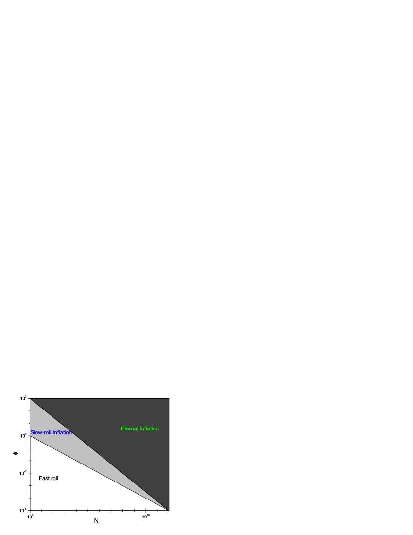
Figure 1: The figure of $\log$ change of the end point of slow roll inflation and the critical point separating the slow roll inflation region and eternal inflation region with respect to the number $N$ of fields in Nflation model with massive fields, in which $m=10^{-6}M_{p}$ is taken. Three regions separated by both lines have been pointed out in figure. We can see that when $N\sim 10^{12}$, the slow roll inflation region disappears.

II.2 The case with mass distribution following Mar$\check{c}$enko-Pastur law

Then we will study a general case with mass distribution following Mar$\check{c}$enko-Pastur law proposed by R. Easther and L. McAllister [5], which appears for axions in string theory. The shape of the mass distribution of axions depends on the basic structure of the mass matrix, which is specified by the supergravity potential. In the simplest assumption, the mass matrix is a random matrix. When one diagonalize this matrix, the fields will be uncoupled with the mass spectrum given by the distribution of eigenvalues. This distribution of the eigenvalues can be characterized by Mar$\check{c}$enko-Pastur law when the matrices are large. The mass distribution taken as the Mar$\check{c}$enko-Pastur law is a function with respect to $\bar{m}$ and $\beta$, where $\bar{m}$ is the average value of the mass, i.e. $<m^{2}>=\bar{m}^{2}$, and $\beta$ is determined by the ratio of the number of axions to the dimension of the moduli space and a model dependent parameter, whose favourable value is expected to be about $0.5$, see Refs. [5, 7]. In this case, the smallest and largest mass are given by $m_{1}^{2}=a\equiv\bar{m}^{2}(1-\sqrt{\beta})^{2}$ and $m_{N}^{2}=b\equiv\bar{m}^{2}(1+\sqrt{\beta})^{2}$, respectively.

In the slow roll approximation, the field value can be given by

$$\phi_{i}(t)\simeq\phi_{i}(t_{0})[\tau(t)]^{m_{i}^{2}\over b},$$ (8)

where $\tau(t)$ is the ratio of the value of the heaviest field at time $t$ to its initial value $t_{0}$, $\tau(t)\equiv{\phi_{N}(t)\over\phi_{N}(t_{0})}$. Then defining $c\equiv{2\ln{[\tau(t)]}\over b}$, the parts including $\phi^{2}_{i}$ in the summation terms of Eqs. (3) and (4) can be replaced with $\phi_{i}^{2}(t_{0})\exp{[cm^{2}_{i}]}$. When we ignore correlations between the mass distribution and the initial field distribution, we can straightly calculate their respective average values. By using power series expansions, the average value of exponential term $\exp{[cm^{2}_{i}]}$ can be written as

$$<\exp{[cm^{2}_{i}]}>=\sum_{i}<m_{i}^{2j}>{c^{j}\over j!}.$$ (9)

The expectation value inside of summation in left hand side of Eq. (9), can be expressed with Narayana numbers $T(i,j)$ (see Eq. (6.14) in Ref. [5])

$$<m_{k}^{2i}> = \bar{m}^{2i}\sum_{j=1}^{i}T(i,j)\beta^{j-1}$$ (10)

$$= \bar{m}^{2i}{{}_{2}{F}_{1}(1-i,-i,2,\beta)},$$

where ${}_{2}F_{1}$ is hypergeometric function. Then Eq. (9) can be rewritten as

$$<\exp[cm_{k}^{2}]>=\sum_{i=0}^{\infty}\bar{m}^{2i}{{}_{2}{F}_{1}(1-i,-i,2,\beta)}{c^{i}\over i!}.$$ (11)

Therefore the summations terms in Eq. (3) with the expectation values of initial conditions and of distribution of mass spectrum of fields are

$$\sum_{i}m_{i}^{2}\phi_{i}^{2}=N\alpha\bar{m}^{2}\sum_{i=0}^{\infty}\bar{m}^{2i}{{}_{2}{F}_{1}(-i,-i-1,2,\beta)}{c^{i}\over i!},$$ (12)

$$\sum_{i}m_{i}^{4}\phi_{i}^{2}=N\alpha\bar{m}^{4}\sum_{i=0}^{\infty}\bar{m}^{2i}{{}_{2}{F}_{1}(-i-1,-i-2,2,\beta)}{c^{i}\over i!},$$ (13)

where $\alpha\equiv<\phi_{i}^{2}(t_{0})>$.

Thus the Eq. (3) with the help of Eqs. (12) and (13) becomes

$$\alpha\simeq{M_{p}^{3}\over{\bar{m}}N^{3\over 2}}f_{1}(t,\beta),$$ (14)

where

$$f_{1}(t,\beta)={\left[\sum_{i=0}^{\infty}\bar{m}^{2i}{{}_{2}{F}_{1}(-i-1,-i-2,2,\beta)}{c^{i}\over i!}\right]^{1/2}\over\left[\sum_{j=0}^{\infty}\bar{m}^{2j}{{}_{2}{F}_{1}(-j,-j-1,2,\beta)}{c^{j}\over j!}\right]^{3/2}},$$ (15)

whose dependence on different $c$ is plotted in Fig. 2. We see that $f_{1}(t,\beta)$ is approximately a constant with order one for a wide range of $c$, i.e. different initial conditions and values of fields. Further, we can note that when all fields have equal values and masses, $f_{1}(t,\beta)$ will have the value $f_{1}(t,\beta)\simeq 1$ with $\alpha\equiv\phi^{2}$ and ${\bar{m}}=m$. In this case Eq. (14) will be exactly same as Eq. (5).

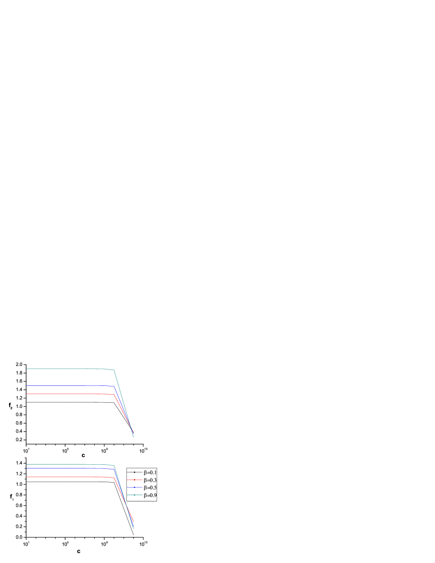
Figure 2: The figures of $f_{1}(t,\beta)$ and $f_{2}(t,\beta)$ with respect to $c$ with different $\beta$. The average mass $\bar{m}=10^{-6}M_{p}$ is taken.

The Eq. (4) with the help of Eqs. (12) and (13) becomes

$$\alpha\simeq{M_{p}^{2}\over N}f_{2}(t,\beta),$$ (16)

where

$$f_{2}(t,\beta)={\left[\sum_{i=0}^{\infty}\bar{m}^{2i}{{}_{2}{F}_{1}(-i-1,-i-2,2,\beta)}{c^{i}\over i!}\right]\over\left[\sum_{j=0}^{\infty}\bar{m}^{2j}{{}_{2}{F}_{1}(-j,-j-1,2,\beta)}{c^{j}\over j!}\right]^{2}},$$ (17)

whose dependence on different $c$ is also plotted in Fig. 2. We see that similar to $f_{1}(t,\beta)$, $f_{2}(t,\beta)$ is also approximately a constant with order one for a wide range of $c$. When all fields have equal values and masses, $f_{2}(t,\beta)\simeq 1$ with $\alpha\equiv\phi^{2}$. In this case Eq. (16) will be exactly same as Eq. (6).

Thus combining Eqs. (14) and (16) to cancel $\alpha$, we have $N\simeq{M_{p}^{2}\over{\bar{m}}^{2}}$, where the ratio of $f_{1}(t,\beta)$ to $f_{2}(t,\beta)$ has been taken as roughly 1, which can be seen in Fig. 2. This is a point in which the slow roll inflation region will disappear. Thus to have a period of slow roll Nflation, the number of fields must be bounded by

$$N\lesssim{M_{p}^{2}\over{\bar{m}}^{2}}.$$ (18)

This result further validates the argument in previous subsection, only replace $m$ with $\bar{m}$.

III The case of Nflation with $\phi^{4}$ fields

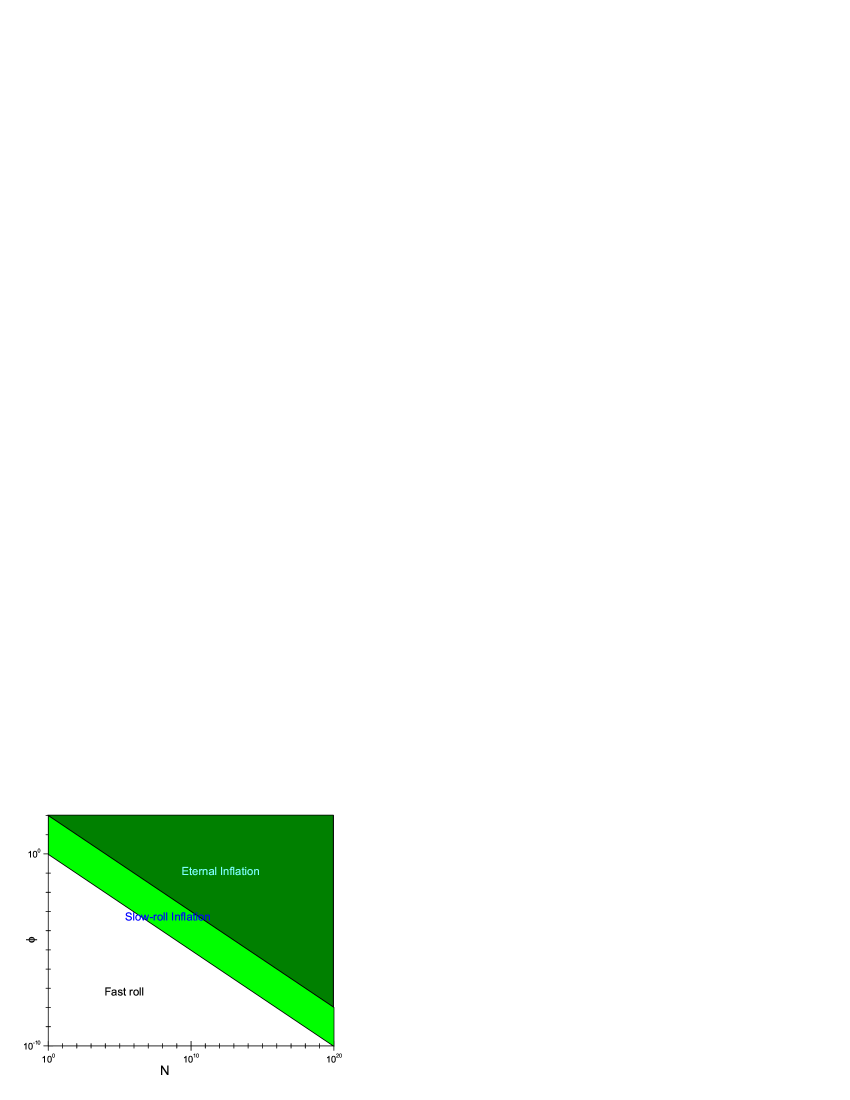
Figure 3: The figure of $\log$ change of the end point of slow roll inflation and the critical point separating the slow roll inflation region and eternal inflation region with respect to the number $N$ of fields in Nflation model with $\phi^{4}$ fields, in which $\lambda=10^{-12}$ is taken. Three regions separated by both lines have been pointed out in figure. We can see that both lines are parallel, thus there is not the bound for $N$.

It is interesting to further check whether there is similar bound for the field number of Nflation with $\phi^{4}$ fields. Following the same steps as we did in the previous section, the critical point separating the slow roll inflation region and eternal inflation region and the end point of inflation can be given by

$$\left(\sum_{i}{\lambda_{i}\phi^{4}_{i}}\right)^{3}\simeq{M_{p}^{6}\over N}\sum_{i}(\lambda_{i}\phi^{3}_{i})^{2},$$ (19)

$$M_{p}^{2}\sum_{i}(\lambda_{i}\phi_{i}^{3})^{2}\simeq\left(\sum_{i}\lambda_{i}\phi_{i}^{4}\right)^{2},$$ (20)

respectively, where $\lambda_{i}$ is the couple constant of the corresponding field and the factors with order one have been neglected. For simplicity, we take all $\phi_{i}=\phi$ and $\lambda_{i}=\lambda$, and thus have

$$\phi\simeq{M_{p}\over\lambda^{{1\over 6}}\sqrt{N}},$$ (21)

$$\phi\simeq{M_{p}\over\sqrt{N}}.$$ (22)

Thus in this case the critical point and the end point approximately obey the same evolution with $N$ increased, which is plotted in Fig.3. This suggests that there is not the bound for the number of fields imposed by the occurrence of slow roll inflation.

This result seems unexpected. The reason leading to it may be that for $\phi^{4}$ field, its effective mass is $\sim\lambda\phi^{2}$, which is changed with $\phi$, and its change in some sense sets off the fast moving of the critical point. When writing $\lambda\phi^{2}=m^{2}$ in Eq. (21), one can find that the resulting equation will be the same as Eq. (5). Thus combining it with Eq. (22), we will have the same result with Eq. (7), which in turn suggests

$$\lambda\phi^{2}\lesssim{M_{p}^{2}\over N}.$$ (23)

Thus for $\phi^{4}$ field, the bound relation between the mass $m$ and $N$ in Eq. (7) for massive field is transferred to that between the field value $\phi$ and $N$. The study with general case will be expected to have approximately the same result with Eq. (23), which is neglected here.

IV Summary and Discussion

In this paper, we study the Nflation model, in which a collection of massive scalar fields drives simultaneously the inflation. We observe that with the increase of fields number, both the critical point separating the slow roll inflation region and eternal inflation region and the end point of slow roll inflation will move towards smaller average value of fields, however, at different rates. In general, the critical point moves faster than the end point, which leads to that the slow roll inflation region will be eat off by the eternal inflation region inch by inch. When the number of fields is enough large, i.e. $N\simeq M_{p}^{2}/{\bar{m}}^{2}$, both points overlaps, which means that the slow roll inflation region completely disappears. In this sense, in order to make Nflation responsible for our observable universe, the field number driving the Nflation must be bounded by $N\lesssim M_{p}^{2}/{\bar{m}}^{2}$.

Recently, it was shown that in theories with a large number $N$ of fields with a mass scale $m$, black hole physics imposes a bound between $M_{p}$ and $N$ [20, 21], i.e. $Nm^{2}\lesssim M_{p}^{2}$, which is actually the same as the result showed here. This can be explained as follows. In general each field can contribute the factor $\sim m^{2}$ into the renormalization of the Planck mass, thus after the accidental cancellations are neglected, the net contribution of $N$ fields will be $\sim Nm^{2}\simeq M_{p}^{2}$. This indicates that with $N$ massive fields there exists a gravitational cutoff, beyond which the quantum gravity effect will become important [22]. When we focus on the inflation driven by $N$ massive fields, we observe that the same cutoff will also appear in a similar sense, i.e. beyond this cutoff the quantum effect will be dominated, it is which that leads to the disappearance of the slow roll inflation region. Thus in this sense our result also justifies the bound of Ref. [20] from a different point of view. In this case exactly the Plank mass should be replaced by renormalized one, i.e. ${\tilde{M}}_{p}^{2}$, which includes the contributions of all massive fields for $M_{p}^{2}$. However, it can be noted that ${\tilde{M}}_{p}^{2}$ is actually the same order as $M_{p}^{2}$. Thus when the renormalization of $M_{p}^{2}$ is considered, our result is not qualitatively altered.

However, this bound can not be applied to nearly massless scalar field. The reason is when the masses of fields are negligible, they will not appear in summation for fields in both sides of Eqs.(3) and (4), which is actually also a reflection that the massless fields do not affect the motion of massive fields dominating the evolution of universe, while the perturbations summed in Eq.(2) are those along the trajectory of fields space, since the massless fields only provide the entropy perturbations orthogonal to the trajectory, which thus are not considered. The same case can be also seen in argument of [20], since the contribution of field to the renormalization of the Planck mass is proportional to $m^{2}$, thus the net contribution leaded by all massless fields to the Planck mass may actually be neglected. Thus if there are some nearly massless fields and some massive fields with nearly same order, it should be that there is a bound $N\lesssim M_{p}^{2}/{\bar{m}}^{2}$, in which only massive fields are included in the definition of $\bar{m}$ and $N$. In our example when the mass distribution is characterized by Mar$\check{c}$enko-Pastur law, as has been used, in which the smallest and largest mass are given by $m_{1}^{2}=\bar{m}^{2}(1-\sqrt{\beta})^{2}$ and $m_{N}^{2}=\bar{m}^{2}(1+\sqrt{\beta})^{2}$, respectively, the masses of all fields are approximately in same order for $\beta\simeq 0.5$. In this case it is natural that all fields need to be considered.

The field $\lambda\phi^{4}$ in essence is different from massive field $m^{2}\phi^{2}$. The former corresponds to have a running mass $\sim\lambda\phi^{2}$, which is dependent of $\phi$. In this case, following Ref. [20], the net contribution of $N$ fields to the renormalization of the Planck mass will be $\sim N\lambda\phi^{2}\simeq M_{p}^{2}$. Thus a same bound relation with Eq.(23) can be obtained, which is seemingly one between the field value $\phi$ and $N$. Eq.(23) can be written as

$$\phi\lesssim{M_{p}\over\sqrt{\lambda N}}.$$ (24)

Note that for general $\lambda<1$, when there is a slow roll inflation region, Eq.(24) is always satisfied, since the inequality given by Eq.(19) is actually included in Eq.(24). Thus it seems that there is not a bound for $N$ in the Nflation with $\lambda\phi^{4}$.

In principle, the bound showed here seems be only valid for massive scalar fields. Further, whether there are similar bounds for other fields with various potentials remains open, and needs to be studied. Be that as it may, however, the result observed, that there may be a large N transition leaded by the quantum effect in inflation, may be interesting, which might have deep relations with other large N phenomena discussed, and thus is worth further explore.

Acknowledgments

We thank S.A. Kim for a kindly help on relevant details in II.B and also Y.F. Cai for helpful comments and discussions. I.A thanks the support of (HEC) Pakistan. This work is supported in part by NSFC under Grant No: 10491306, 10521003, 10775179, 10405029, 10775180, in part by the Scientific Research Fund of GUCAS(NO.055101BM03), in part by CAS under Grant No: KJCX3-SYW-N2.

References

- [1] A.R. Liddle, A. Mazumdar, and F.E. Schunck, Phys. Rev. D58, 061301 (1998).
- [2] K.A. Malik and D. Wands, Phys. Rev. D59, 123501 (1999); E.J. Copeland, A. Mazumdar and N.J. Nunes, Phys. Rev. D60, 083506 (1999); A.M. Green and J.E. Lidsey, Phys. Rev. D61, 067301 (2000); A. Mazumdar, S. Panda and A. Perez-Lorenzana, Nucl. Phys. B614, 101 (2001); P. Kanti and K.A. Olive, Phys. Rev. D60, 043502 (1999); Phys. Lett. B464, 192 (1999); N. Kaloper and A.R. Liddle Phys. Rev. D61, 123513 (2000); Y.S. Piao, W. Lin, X. Zhang and Y.Z. Zhang, Phys. Lett. B528, 188 (2002).
- [3] Y.S. Piao, R.G Cai, X. Zhang and Y.Z. Zhang Phys. Rev. D66, 121301 (2002); M. Majumdar and A.C. Davis Phys. Rev. D69, 103504 (2004); R. Brandenberger, P. Ho and H. Kao, JCAP 0411, 011 (2004) ; A. Jokinen and A. Mazumdar, Phys. Lett. B597, 222 (2004); K. Becker, M. Becker and A. Krause, Nucl. phys. B715 (2005) 349-371; J.M. Cline and H. Stoica, Phys. Rev. D72, 126004 (2005); J. Ward, Phys. Rev. D73, 026004 (2006); H. Singh, arXiv:hep-th/0608032.
- [4] S. Dimopoulos, S. Kachru, J. McGreevy, and J.G. Wacker, arXiv:hep-th/0507205.
- [5] R. Easther and L. McAllister, JCAP 0605, (2006) 018.
- [6] S.A. Kim and A.R. Liddle, Phys. Rev. D74, 023513 (2006).
- [7] S.A. Kim and A.R. Liddle, arXiv:0707.1982.
- [8] Y.S. Piao, Phys. Rev. D74, (2006) 047302.
- [9] I. Ahmad, Y.S. Piao, C.F. Qiao, JCAP 02, 002 (2008).
- [10] L. Alabidi, and D.H. Lyth, JCAP 0605, 016 (2006).
- [11] S.A. Kim and A.R. Liddle, Phys. Rev. D74, 063522 (2006).
- [12] D. Battefeld, T. Battefeld, JCAP 0705, 012 (2007).
- [13] D. Seery, J.E. Lidsey, M.S. Sloth, JCAP 0701, 027 (2007); D. Seery, J.E. Lidsey, JCAP 0701, 008 (2007); T. Battefeld, R. Easther, JCAP 0703, 020 (2007); J.O. Gong, Phys. Rev. D75, 043502 (2007); M.E. Olsson, JCAP 0704, 019 (2007); K.L. Panigrahi, H. Singh, arXiv:0708.1679; J. Ward, arXiv:0711.0760.
- [14] A. Vilenkin, Phys. Rev. D27, 2848 (1983).
- [15] A.D. Linde, Phys. Lett. B175, 395 (1986).
- [16] A.A. Starobinsky, in “Current Topics in Field Theory, Quantum Gravity and Strings,” edited by H.J. de Vega and N. Sanchez, Lecture Notes in Physics, Vol.26 (Springer, Heidelberg, 1986), 107.
- [17] A.S. Goncharov, A.D. Linde, V.F. Mukhanov, Int. J. Mod. Phys. A2, 561 (1987).
- [18] A.D. Linde, “Particle Physics and Inflationary Cosmology”, (Harwood, Chur, Switzerland, 1990); Contemp. Concepts Phys. 5, 1 (2005), arXiv:hep-th/0503203.
- [19] A.D. Linde, Nucl. Phys. B372, 421 (1992).
- [20] G. Dvali, arXiv:0706.2050.
- [21] G. Dvali, D. Lust, arXiv:0801.1287.
- [22] G. Dvali, M. Redi, arXiv:0710.4344.