Tachyon Condensation on Separated Brane-Antibrane System

Arjun Bagchi and Ashoke Sen

Harish-Chandra Research Institute

Chhatnag Road, Jhusi, Allahabad 211019, INDIA

E-mail: arjun@hri.res.in, sen@hri.res.in

Abstract

We study the effect of tachyon condensation on a brane antibrane pair in superstring theory separated in the transverse direction. The static properties of the tachyon potential analyzed using level truncated string field theory reproduces the desired property that the dependence of the minimum value of the potential on the initial distance of separation between the branes decreases as we include higher level terms. The rolling tachyon solution constructed using the conformal field theory methods shows that if the initial separation between the branes is less than a critical distance then the solution is described by an exactly marginal deformation of the original conformal field theory where the correlation functions of the deformed theory are determined completely in terms of the correlation functions of the undeformed theory without any need to regularize the theory. Using this we give an expression for the pressure on the brane-antibrane system as a power series expansion in $\exp(Cx^{0})$ for an appropriate constant $C$.

1 Introduction

The spectrum of the bosonic open string theory living on a D-brane is known to have a tachyonic mode. We now have a good understanding of the physics around the minimum of the tachyon potential, both via conformal field theory (CFT) methods[1], and numerical and analytical methods in string field theory[2, 3, 4, 5, 6, 7, 8, 9, 10, 11, 12, 13, 14, 15, 16, 17]. In particular it is known that the tachyon potential has a non-trivial minimum where the energy density from the potential exactly equals the negative of the D-brane tension and as a result the sum vanishes. The minimum represents a vacuum without any D-branes. Using conformal field theory methods one can also study time dependent solutions in string theory describing the rolling of the tachyon towards the vacuum[18].

Similar conjectures hold in the case of the superstrings where tachyonic modes appear in unstable systems like non-BPS D-branes or brane-antibrane pairs[19]. Level truncation gives numerical evidence for these conjectures in Berkovits superstring field theory[20, 21, 22, 23], but as of now we do not have an analytic solution for the vacuum. As in the case of bosonic string theory, one can also construct a conformal field theory describing the rolling of the tachyon towards the vacuum[25].

Most of the work on tachyon condensation in superstring field theory has been carried out on an unstable D-brane system, or a closely related system containing a coincident brane-antibrane pair. In this paper, we look at a system of brane-antibrane pair separated by a distance $d$. This is the configuration we expect to get in any realistic situation involving tachyon condensation on a brane-antibrane system, e.g. in cosmology, where the brane-antibrane pair would start out separated from each other and gradually come together by gravitational attraction[26]. As they come closer than the critical distance the lowest lying mode of the open string stretched between the brane and the antibrane will become tachyonic and the condensation process would start. Thus if we want to study the end point of tachyon condensation for such a system we need to study tachyon condensation on a separated brane-antibrane pair.

Our analysis will be divided into two parts. We first look at the static configuration of a separated brane-antibrane pair, and carry out a level truncation analysis of the tachyon vacuum using Berkovits’ superstring field theory[27, 28]. In this case we do not expect any surprise; rather we expect that at the bottom of the potential the total energy density should continue to vanish irrespective of the initial distance between the brane-antibrane pair. This result is bourn out by our analysis. In particular we find that while at the lowest level the value of the potential at the minimum depends on the initial separation between the brane-antibrane pair, this dependence reduces after inclusion of higher level terms in the action.

The second part of the analysis involves study of the rolling tachyon solution using conformal field theory method. Unlike in the case of rolling tachyon on a non-BPS D-brane or a coincident brane-antibrane pair, in this case we cannot construct an exact boundary state corresponding to the time dependent configuration. Nevertheless using a perturbative approach one can write down an expression for the pressure as a series expansion in powers of $\exp(Cx^{0})$ for an appropriate constant $C$ depending on the initial separation of the brane-antibrane system. We find that if the initial separation between the brane-antibrane pair is less than a critical distance then the coefficients of the various terms of the expansion can be expressed in terms of non-singular integrals. We analyze the behaviour of this series by computing the first few terms in the expansion numerically.

For rolling tachyon solution on a coincident brane-antibrane pair the final state was found to have vanishing pressure but non-zero energy density[25]. This reflects that the final state is made of non-relativistic heavy closed string states[29, 30]. If instead of starting with a coincident brane-antibrane pair we begin with a separated brane-antibrane pair then the final state in principle could be different, (say) consisting of a mixture of non-relativistic heavy closed string states and radiation containing relativistic light closed string states. Thus computation of the final state pressure is an important problem since this could tell us indirectly about the composition of the final state. Unfortunately since we only have a power series expansion for the pressure, we cannot reach a definite conclusion about the final state pressure. However we use the Pade approximant method to represent the known results on the power series expansion as a ratio of polynomial functions, and extrapolate the result based on the first few coefficients to study the behaviour of the pressure at large time. This naive extrapolation gives results consistent with vanishing pressure at late time.

During our analysis we also develop a general procedure for studying rolling tachyon solution in situations where the tachyon vertex operator is a non-trivial matter primary operator. We find that as long as the tachyon is sufficiently tachyonic, ı.e. the tachyon mass² is below a critical value, the system admits an exactly marginal deformation describing the rolling of the tachyon away from the maximum. The essential point is that the integrated vertex operator describing a rolling tachyon deformation, obtained by multiplying the zero momentum tachyon vertex operator by $e^{CX^{0}}$ for an appropriate constant $C$, has non-singular operator product with itself for sufficiently large $C$. As a result deformation by this operator describes an exactly marginal deformation of the conformal field theory.

2 Superstring field theory on brane-antibrane system

In this section we give a quick review of the construction of the superstring field theory (SSFT) on a brane antibrane pair. We then identify the specific components of the string field which we shall use for the study of tachyon condensation on a separated brane-antibrane pair.

2.1 SSFT on a BPS D-brane

We begin by looking at the GSO(+) sector of the superstring field theory which describes the dynamics of the NS sector of open strings living on a single BPS D-brane. The CFT describing the first quantized open string theory is a direct product of superconformal matter with $c=15$ containing the fields $X^{\mu}$, $\psi^{\mu}$ for $0\leq\mu\leq 9$, and $b$, $c$, $\beta$, $\gamma$ ghost CFT with $c=-15$. The $\beta$, $\gamma$ system can be reexpressed in terms of the bosonised ghosts $\xi$, $\eta$ and $\phi$ with[31]

$$\beta={\partial\xi}e^{-\phi},\quad\gamma=\eta e^{\phi}\,.$$ (2.1)

We shall be working in the large Hilbert space which includes the zero mode of the field $\xi$ and use the convention set in [21]. We normalize the various fields so that the leading singularities in the various operator product expansions have the following form

$$\partial X^{\mu}(z)\partial X^{\nu}(w)\simeq-{1\over 2}\eta^{\mu\nu}(z-w)^{-2}$$

$$\partial\phi(z)\partial\phi(w)\simeq-(z-w)^{-2}$$

$$\psi^{\mu}(z)\psi^{\nu}(w)\simeq\eta^{\mu\nu}\,(z-w)^{-1}$$

$$\xi(z)\eta(w)\simeq(z-w)^{-1}$$

$$b(z)c(w)\simeq(z-w)^{-1}$$

$$e^{\alpha\phi(z)}e^{\beta\phi(w)}\simeq(z-w)^{-\alpha\beta}e^{(\alpha+\beta)w},\quad z,w\in{\hbox{ C\kern-5.69054ptC}}$$

$$e^{ik_{1}\cdot X(s)}e^{ik_{2}\cdot X(s^{\prime})}\simeq|s-s^{\prime}|^{-2k_{1}\cdot k_{2}}e^{i(k_{1}+k_{2})\cdot X(s^{\prime})},\quad s,s^{\prime}\in{\hbox{ R\kern-6.82864ptR}}\,.$$ (2.2)

We shall denote by $\langle\prod_{i}A_{i}\rangle$ the correlation functions in the combined matter-ghost boundary CFT (BCFT) on the unit disk with vertex operators $A_{i}$ inserted on the boundary. The correlation functions are normalized as

$$<\xi(z)c\partial{c}\partial^{2}c(w)e^{-2\phi(y)}>=2\,.$$ (2.3)

The BRST operator is given by:

$$Q_{B}=\oint dzj_{B}(z)=\oint dz\{c(T_{m}+T_{\xi\eta}+T_{\phi})+c\partial{c}b+\eta e^{\phi}G_{m}-\eta\partial{\eta}e^{2\phi}b\}$$ (2.4)

where the $T$’s denote the energy momentum tensors for the various fields and $G_{m}$ is the matter superconformal generator:

$$T_{m} = -(\partial X^{\mu}\partial X_{\mu}+\frac{1}{2}\psi^{\mu}\partial\psi_{\mu})$$

$$G_{m} = -i\sqrt{2}\,\psi_{\mu}\partial X^{\mu}$$

$$T_{\xi\eta} = \partial{\xi}{\eta}$$

$$T_{\phi} = -\frac{1}{2}\partial\phi\partial\phi-\partial^{2}\phi\,.$$ (2.5)

The Berkovits’ superstring field theory action is given by

$$S=\frac{1}{2g^{2}}\left\langle\left\langle(e^{-\Phi}Q_{B}e^{\Phi})\left(e^{-\Phi}{\eta}_{0}e^{\Phi}\right)-\int_{0}^{1}dte^{-t\Phi}\partial_{t}e^{t\Phi}\left\{e^{-t\Phi}Q_{B}e^{t\Phi},e^{-t\Phi}{\eta}_{0}e^{t\Phi}\right\}\right\rangle\right\rangle$$ (2.6)

where the string field $\Phi$ is a ghost number zero and picture number 0 state of the CFT in the large Hilbert space and the action needs to be defined by expanding (2.6) in a power series in $\Phi$ and carefully preserving the order of the operators. The notation $\langle\langle~{}\rangle\rangle$ means

$$\langle\langle A_{1}A_{2}...A_{n}\rangle\rangle=\langle f_{1}^{(n)}\circ A_{1}(0)f_{2}^{(n)}\circ A_{2}(0)...f_{n}^{(n)}\circ A_{n}(0)\rangle$$ (2.7)

with $f_{l}^{(n)}\circ A_{l}$ implying the conformal transformation of the operator $A_{l}$ under the map $f_{l}^{(n)}$. The maps $f_{l}^{(n)}$ are given by

$$f_{l}^{(n)}(z)=e^{(2\pi i(l-1))/n}\left(\frac{1+iz}{1-iz}\right)^{2/n}$$ (2.8)

2.2 SSFT on a non-BPS D-brane

In order to extend this formalism to non-BPS D-branes one needs to take into account the GSO($-$) sector that now comes into the picture. In order to keep the basic algebraic framework unchanged, one introduces internal Chan-Paton (CP) factors and performs a trace over them. The GSO(+) sector states carry CP factor proportional to the $2\times 2$ identity matrix $I$ whereas the GSO($-$) sector states carry CP factor proportional to the Pauli matrix $\sigma_{1}$. Consequently, the complete string field $\widehat{\Phi}$ is now represented by

$$\widehat{\Phi}=\Phi_{+}\otimes I+\Phi_{-}\otimes\sigma_{1}\,.$$ (2.9)

We also need to modify the $Q_{B}$ and $\eta_{0}$ operators by tensoring them with CP factor $\sigma_{3}$

$$\widehat{Q}_{B}=Q_{B}\otimes\sigma_{3},\hskip 5.69054pt\widehat{\eta}_{0}=\eta_{0}\otimes\sigma_{3}\,.$$ (2.10)

In computing the double bracket $\langle\langle~{}\rangle\rangle$ of hatted operators we need to take the trace over the internal CP factors:

$$\langle\langle\widehat{A}_{1}\widehat{A}_{2}...\widehat{A}_{n}\rangle\rangle=Tr\langle f_{1}^{(n)}\circ\widehat{A}_{1}(0)f_{2}^{(n)}\circ\widehat{A}_{2}(0)...f_{n}^{(n)}\circ\widehat{A}_{n}(0)\rangle\,.$$ (2.11)

The Berkovits’ action looks almost the same, with all the fields and operators replaced by hatted fields and operators respectively. We also divide the action by an extra factor of 2 in order to compensate for the factor of 2 coming from the trace over the internal CP factors:

$$S=\frac{1}{4g^{2}}\left\langle\left\langle\left((e^{-\widehat{\Phi}}Q_{B}e^{\widehat{\Phi}})(e^{-\widehat{\Phi}}{\eta}_{0}e^{\widehat{\Phi}})-\int_{0}^{1}dte^{-t\widehat{\Phi}}\partial_{t}e^{t\widehat{\Phi}}\{e^{-t\widehat{\Phi}}Q_{B}e^{t\widehat{\Phi}},e^{-t\widehat{\Phi}}{\eta}_{0}e^{t\widehat{\Phi}}\}\right)\right\rangle\right\rangle$$ (2.12)

2.3 SSFT on a D-brane-$\bar{\rm D}$-brane pair

The formalism needs to be further modified in order to extend it to the brane-antibrane system. Here besides the internal CP factors like the ones used for the non-BPS branes one also needs to use external CP factors. There are four kinds of strings represented by the external CP matrices:

$$A:\left(\begin{array}[]{cc}1&0\\ 0&0\end{array}\right)\>,\quad\>B:\left(\begin{array}[]{cc}0&0\\ 0&1\end{array}\right)\>,\quad\>C:\left(\begin{array}[]{cc}0&1\\ 0&0\end{array}\right)\>,\quad\>D:\left(\begin{array}[]{cc}0&0\\ 1&0\end{array}\right).$$

The strings on the individual branes are represented by the CP factors $A$, $B$ or equivalently by $I$ and $\sigma_{3}$. These are in the GSO(+) sector. The GSO($-$) states are the ones which live on the strings stretched between the brane and the antibrane, – they are represented by the CP factors $C$, $D$ or equivalently by $\sigma_{1}$, $\sigma_{2}$. The complete string field $\widehat{\Phi}$ now reads

$$\widehat{\Phi}=\left(\Phi_{+}^{(1)}\otimes I+\Phi_{+}^{(2)}\otimes\sigma_{3}\right)\otimes I+\left(\Phi_{-}^{(3)}\otimes\sigma_{1}+\Phi_{-}^{(4)}\otimes\sigma_{2}\right)\otimes\sigma_{1}\,.$$ (2.13)

We follow the convention that the external CP factor will be written first followed by the internal CP factor.

The $\widehat{Q}_{B}$ and $\widehat{\eta}_{0}$ operators are now given by

$$\widehat{Q}_{B}=Q_{B}\otimes I\otimes\sigma_{3},\hskip 5.69054pt\widehat{\eta}_{0}=\eta_{0}\otimes I\otimes\sigma_{3}\,.$$ (2.14)

The double brackets $\langle\langle~{}\rangle\rangle$ are now defined with a double trace, over both internal and external CP factors:

$$\langle\langle\widehat{A}_{1}\widehat{A}_{2}\ldots\widehat{A}_{n}\rangle\rangle=Tr_{ext}\otimes Tr_{int}\langle f_{1}^{(n)}\circ\widehat{A}_{1}(0)f_{2}^{(n)}\circ\widehat{A}_{2}(0)...f_{n}^{(n)}\circ\widehat{A}_{n}(0)\rangle\,.$$ (2.15)

The action looks very much the same as for the non-BPS D-brane except that we divide by a further factor of 2 to compensate for the trace over the external Chan-Paton factors:

$$S=\frac{1}{8g^{2}}\left\langle\left\langle\left((e^{-\widehat{\Phi}}Q_{B}e^{\widehat{\Phi}})(e^{-\widehat{\Phi}}{\eta}_{0}e^{\widehat{\Phi}})-\int_{0}^{1}dte^{-t\widehat{\Phi}}\partial_{t}e^{t\widehat{\Phi}}\{e^{-t\widehat{\Phi}}Q_{B}e^{t\widehat{\Phi}},e^{-t\widehat{\Phi}}{\eta}_{0}e^{t\widehat{\Phi}}\}\right)\right\rangle\right\rangle\,.$$ (2.16)

We shall find it convenient to consider the time direction as a circle with unit period. The tachyon potential would then just be the negative of the action for static configurations. With this normalization the total tension of the brane-antibrane pair is given by

$$T={1\over 2\pi^{2}g^{2}}\,.$$ (2.17)

For explicit calculations, it is useful to expand the action in a formal power series in $\widehat{\Phi}$. It can be arranged in the form[21]

$$S=\frac{1}{4g^{2}}\sum_{M,N=0}^{\infty}\frac{(-1)^{N}}{(M+N+2)!}\left({M+N\atop N}\right)\left\langle\left\langle\left(\widehat{Q}_{B}\widehat{\Phi}\right)\widehat{\Phi}^{M}\left(\widehat{\eta}_{0}\widehat{\Phi}\right)\widehat{\Phi}^{N}\right\rangle\right\rangle\,.$$ (2.18)

2.4 Separated D-branes

Our interest is in a configuration where the brane and the antibrane are separated from each other. In this case the mass of any state of the string stretched between the brane and the antibrane gets an additional contribution from the tension of the string compared to the string whose both ends are on the same brane. If we denote by $d^{\prime}$ the separation between the brane and the antibrane then in the $\alpha^{\prime}=1$ unit this additional contribution, affecting the formula for the mass² in sectors C and D, is given by $d^{\prime 2}/4\pi^{2}$. Consequently the vertex operators in the GSO($-$) sector, which represent the states of string stretching between the brane and the anti-brane, gets an additional piece that reflects the effect of the winding charge that the string carries due to the stretching between the branes. If we denote by $Y$ the world-sheet scalar along the direction of separation and if $\widetilde{Y}$ denotes the field dual to $Y$ then the additional piece in the vertex operator is given by

$$\Delta=e^{\pm id^{\prime}\widetilde{Y}/2\pi}=e^{\pm id\widetilde{Y}}$$ (2.19)

where $d=d^{\prime}/2\pi$ and the $+$ and $-$ signs refer to sectors C and D respectively.

We shall now describe the off-shell vertex operators associated with the string field components we use in the level truncation analysis. First of all we have the tachyon vertex operator. For the non-BPS D-brane, the zero momentum tachyon vertex operator is given by

$$\widehat{V}_{T}=\xi ce^{-\phi}\otimes\sigma_{1}\,.$$ (2.20)

On a separated brane-antibrane pair the tachyon vertex operator must carry the factors given in (2.19). Since we require that the tachyon that condenses is real, the vertex operator must be hermitian. This gives

$$\widehat{V}_{T} = \xi ce^{-\phi}e^{id\widetilde{Y}}\otimes\pmatrix{0&1\cr 0&0}\otimes\sigma_{1}+\xi ce^{-\phi}e^{-id\widetilde{Y}}\otimes\pmatrix{0&0\cr 1&0}\otimes\sigma_{1}$$ (2.21)

$$= \pmatrix{0&{\xi ce^{-\phi}e^{id\widetilde{Y}}}\cr\xi ce^{-\phi}e^{-id\widetilde{Y}}&0}\otimes\sigma_{1}\,.$$

$\widehat{V}_{T}$ has total conformal weight $d^{2}-{1\over 2}$. Furthermore we have

$$\widehat{Q}_{B}\widehat{V}_{T} = \left({\left(d^{2}-\frac{1}{2}\right)\xi c\partial{c}e^{-\phi}e^{id\widetilde{Y}}-\frac{d}{\sqrt{2}}\psi_{y}ce^{id\widetilde{Y}}-\eta e^{\phi}e^{id\widetilde{Y}}}\right)\otimes\pmatrix{0&1\cr 0&0}\otimes i\sigma_{2}$$

$$+ \left({\left(d^{2}-\frac{1}{2}\right)\xi c\partial{c}e^{-\phi}e^{-id\widetilde{Y}}+\frac{d}{\sqrt{2}}\psi_{y}ce^{-id\widetilde{Y}}-\eta e^{\phi}e^{-id\widetilde{Y}}}\right)\otimes\pmatrix{0&0\cr 1&0}\otimes i\sigma_{2}\,,$$

$$\widehat{\eta}_{0}\widehat{V}_{T}=\pmatrix{0&{ce^{-\phi}e^{id\widetilde{Y}}}\cr{ce^{-\phi}e^{-id\widetilde{Y}}}&0}\otimes i\sigma_{2}\,,$$ (2.23)

where $\psi_{y}$ is the world-sheet superpartner of $\widetilde{Y}$ on the boundary.

The string field theory action has two ${\hbox{ Z\kern-4.55244ptZ}}_{2}$ symmetries under which the tachyon vertex operator $\widehat{V}_{T}$ is even. The first one corresponds to $Y\to-Y$, $\psi_{y}\to-\psi_{y}$ together with conjugation by the CP factor $\sigma_{1}\times I$. We shall denote the generator of this symmetry by $\sigma$. The second one is the so called ‘twist symmetry’ under which a vertex operator with a conformal weight $h$ from the oscillators (not counting the contribution from the $e^{\pm id\widetilde{Y}}$ factors) picks up a phase of $(-1)^{h+1}$ for integer $h$ and $(-1)^{h+{1\over 2}}$ for half integer $h$, and the Chan-Paton factor associated with this vertex operator gets transposed. We shall accompany this by the $Y\to-Y$, $\psi_{y}\to-\psi_{y}$ transformation so that the tachyon vertex operator $\widehat{V}_{T}$ is even under this transformation. We shall denote the generator of this symmetry by $\tau$. We shall restrict to string field configurations which are even under the $\sigma$ and $\tau$ transformations.

At the next level we have four more string fields associated with the vertex operators

$$\widehat{V}^{(1)}_{K} = \xi ce^{-\phi}\psi_{y}\otimes\pmatrix{1&0\cr 0&-1}\otimes I$$

$$\widehat{V}^{(2)}_{K} = \xi ce^{-\phi}\psi_{y}\otimes\pmatrix{1&0\cr 0&1}\otimes I$$

$$\widehat{V}^{(1)}_{M} = c\partial{c}\xi\partial{\xi}e^{-2\phi}\otimes\pmatrix{1&0\cr 0&-1}\otimes I$$

$$\widehat{V}^{(2)}_{M} = c\partial{c}\xi\partial{\xi}e^{-2\phi}\otimes\pmatrix{1&0\cr 0&1}\otimes I\,,$$ (2.24)

each of conformal weight 0. Of these the vertex operators $\widehat{V}^{(2)}_{K}$ and $\widehat{V}^{(1)}_{M}$ are odd under $\sigma$. Thus we can set the components of the string field along this direction to zero. The vertex operator $\widehat{V}^{(2)}_{M}$ on the other hand is odd under $\tau$. Thus we can set the coefficient of this operator also to zero. As a result we are left with only the vertex operator $\widehat{V}^{(1)}_{K}$ which is even under both $\sigma$ and $\tau$. The field associated with this vertex operator has the interpretation of being the mode that shifts the branes in the opposite direction by a distance proportional to its expectation value.

From eq.(2.4) we get

$$\widehat{Q}_{B}\widehat{V}^{(1)}_{K} = \left(i\,\sqrt{2}\,c\partial{Y}+\eta\psi_{y}e^{\phi}\right)\otimes\pmatrix{1&0\cr 0&-1}\otimes\sigma_{3}\,,$$ (2.25)

$$\widehat{\eta}_{0}\widehat{V}^{(1)}_{K}=ce^{-\phi}\psi_{y}\otimes\pmatrix{1&0\cr 0&-1}\otimes\sigma_{3}\,.$$ (2.26)

3 Tachyon vacuum

Now, with the ingredients prepared, we can apply the method of level truncation to study tachyon condensation on separated branes. We shall use the expanded form (2.18) of the Berkovits’ action to evaluate the relevant terms at various levels. We define the level of a string field component multiplying a vertex operator of conformal weight $h$ to be $h+\frac{1}{2}$ so that the zero momentum tachyon at zero separation between the brane and the antibrane has weight zero.

3.1 Level $d^{2}$ Computation

The only field we need to keep in the analysis at the lowest level ($d^{2}$) is the tachyon field:

$$\widehat{\Phi}=t\widehat{V}_{T}\equiv\widehat{T}\,.$$ (3.1)

In order to get a non-vanishing correlation function the total $\phi$ charge must add up to $-2$. This restricts the form of the pure tachyon potential to the form $at^{2}+bt^{4}$, since terms involving more than four powers of $\widehat{T}$ (ı.e. $M+N>2$ terms in (2.18)) vanish by $\phi$ charge conservation.

From the expanded form (2.18), the quadratic term in the action reads

$$S_{2}=\frac{1}{8g^{2}}\langle\langle(\widehat{Q}_{B}\widehat{T})(\widehat{\eta}_{0}\widehat{T})\rangle\rangle$$ (3.2)

We use (2.4) and (2.23) to write down the form of the two-point function and then compute it using the standard correlation functions on the unit disk:

$$\displaystyle\langle\langle(\widehat{Q}_{B}\widehat{T})(\widehat{\eta}_{0}\widehat{T})\rangle\rangle = 2\left(d^{2}-\frac{1}{2}\right)\bigg{\{}\langle\langle(\xi c\partial{c}e^{-\phi}e^{id\widetilde{Y}})(ce^{-\phi}e^{-id\widetilde{Y}})\rangle\rangle$$ (3.3)

$$\qquad\qquad\qquad+\langle\langle(\xi c\partial{c}e^{-\phi}e^{-id\widetilde{Y}})(ce^{-\phi}e^{id\widetilde{Y}})\rangle\rangle\bigg{\}}\,t^{2}\,.$$

Using

$$\displaystyle\langle\langle(\xi c\partial{c}e^{-\phi}e^{\pm id\widetilde{Y}})(ce^{-\phi}e^{\mp id\widetilde{Y}})\rangle\rangle = (f_{1}^{(2)\prime}(0)f_{2}^{(2)\prime}(0))^{d^{2}-\frac{1}{2}}\langle\xi c\partial{c}e^{-\phi}e^{\pm idX}(1)ce^{-\phi}e^{\mp idX}(-1)\rangle_{\hbox{disk}}$$ (3.4)

$$= -1$$

we get

$$\displaystyle\langle\langle(\widehat{Q}_{B}\widehat{T})(\widehat{\eta}_{0}\widehat{T})\rangle\rangle = -2(2d^{2}-1)t^{2}\,.$$ (3.5)

This gives

$$S_{2}=-{1\over 2g^{2}}\left(d^{2}-{1\over 2}\right)t^{2}\,.$$ (3.6)

The quartic term in the action is

$$S_{4}=-\frac{1}{48g^{2}}\left(\left\langle\left\langle(\widehat{Q}_{B}\widehat{T})\widehat{T}(\widehat{\eta}_{0}\widehat{T})\widehat{T}\right\rangle\right\rangle-\left\langle\left\langle(\widehat{Q}_{B}\widehat{T})\widehat{T}\widehat{T}(\widehat{\eta}_{0}\widehat{T})\right\rangle\right\rangle\right)\,.$$ (3.7)

Here we implicitly used the ”twist symmetry” to simplify the expression. We compute the correlation functions in the same way as above. For example we have

$$\langle\langle(\widehat{Q}_{B}\widehat{T})\widehat{T}(\widehat{\eta}_{0}\widehat{T})\widehat{T}\rangle\rangle=2\left\langle\left\langle(\eta e^{\phi}e^{id\widetilde{Y}})(\xi ce^{-\phi}e^{-id\widetilde{Y}})(ce^{-\phi}e^{id\widetilde{Y}})(\xi ce^{-\phi}e^{-id\widetilde{Y}})\right\rangle\right\rangle$$

$$+2\left\langle\left\langle(\eta e^{\phi}e^{-id\widetilde{Y}})(\xi ce^{-\phi}e^{id\widetilde{Y}})(ce^{-\phi}e^{-id\widetilde{Y}})(\xi ce^{-\phi}e^{id\widetilde{Y}})\right\rangle\right\rangle$$ (3.8)

and a similar expression for $\langle\langle(\widehat{Q}_{B}\widehat{T})\widehat{T}\widehat{T}(\widehat{\eta}_{0}\widehat{T})\rangle\rangle$. The calculation yields

$$g^{2}S_{4}=-\frac{t^{4}}{12}\left(4+2\right)$$ (3.9)

The tachyon potential $V(t,d)$ is just the negative of the action as we have chosen the time coordinate to be periodic with a period 1. This gives

$$V(t,d)=-(S_{2}+S_{4})=\frac{1}{2g^{2}}\left[\left(d^{2}-\frac{1}{2}\right)t^{2}+t^{4}\right]$$ (3.10)

We now minimize the potential with respect to t. This gives

$$\left[(1-2d^{2})-4t^{2}\right]t=0$$ (3.11)

The solution $t_{*}$ to this equation corresponding to the minimum of $V(t,d)$ is

$$t_{*}^{2} = {1\over 4}\,(1-2d^{2})\quad\hbox{for $d^{2}<1/2$}$$ (3.12)

$$t_{*} = 0\quad\hbox{for $d^{2}\geq 1/2$}.$$ (3.13)

For $d^{2}<1/2$, the value of the potential at the minimum is given by:

$$V_{min}=-\frac{1}{32g^{2}}(1-2d^{2})^{2}\,.$$ (3.14)

For $d=0$ eq.(3.10)-(3.14) reduce to

$$V(t,d=0)=\frac{1}{g^{2}}\left(-\frac{1}{4}t^{2}+\frac{1}{2}t^{4}\right)$$

$$t_{*}^{2}=1/4\Rightarrow t_{*}=\pm 1/2$$

$$V_{min}=-\frac{1}{32g^{2}}$$

These are in perfect agreement with the level zero calculations in [20, 21].

3.2 Including the shift field

Next we wish to compute the tachyon potential to the next non-trivial order. At this level we need to include the level ${1\over 2}$ shift field associated with the vertex operator $\widehat{V}_{K}^{(1)}$. Thus the string field has the expansion

$$\widehat{\Phi}=t\widehat{V}_{T}+\chi\widehat{V}^{(1)}_{K}\equiv\widehat{T}+\widehat{K}\,.$$ (3.15)

We shall collect terms in the potential up to level $(1+2d^{2})$. Again all terms with higher than four powers of the string field vanish by $\phi$ charge conservation. Thus we need to examine the terms of order $\chi^{2}$, $t^{2}\chi$ and $t^{2}\chi^{2}$. Explicit computation to this order shows that the coefficient of the $\chi^{2}$ term vanishes and the cubic and quartic terms are given by

$$S_{3}^{\prime}=-{1\over\sqrt{2}\,g^{2}}\,d\,\left(\frac{16}{27}\right)^{d^{2}-\frac{1}{2}}t^{2}\chi\,,$$ (3.16)

$$S_{4}^{\prime}=-\frac{1}{g^{2}}\left(2^{\frac{1}{2}-d^{2}}+2^{-1-2d^{2}}\right)t^{2}\chi^{2}\,.$$ (3.17)

Adding $-S_{3}^{\prime}-S_{4}^{\prime}$ to the previous form of the tachyon potential we get

$$V(t,\chi,d)=\frac{1}{2g^{2}}\left[-\left({\frac{1}{2}-d^{2}}\right)t^{2}+t^{4}+\sqrt{2}d\left(\frac{16}{27}\right)^{d^{2}-\frac{1}{2}}t^{2}\chi+\left(2^{\frac{3}{2}-d^{2}}+2^{-2d^{2}}\right)t^{2}\chi^{2}\right]$$ (3.18)

Eliminating $\chi$ using its equation of motion gives an effective tachyon potential of the form:

$$V_{eff}(t)=\frac{1}{2g^{2}}\left[-\left({\frac{1}{2}-d^{2}}+{1\over 2}d^{2}\left(\frac{16}{27}\right)^{2d^{2}-1}\left(2^{\frac{3}{2}-d^{2}}+2^{-2d^{2}}\right)^{-1}\right)t^{2}+t^{4}\right]\,.$$ (3.19)

From this we see that the effect of the field $\chi$ is to make the tachyon more tachyonic. This is not surprising since we expect that once a tachyon vacuum expectation value is switched on, the field $\chi$ will develop a potential that tries to pull the brane and the antibrane towards each other. This is turn will reduce the tachyon mass². Minimizing the effective potential (3.19) with respect to $t$ now gives

$$V_{min}=-\frac{1}{32g^{2}}\left[1-2d^{2}+d^{2}\left(\frac{16}{27}\right)^{2d^{2}-1}\left(2^{\frac{3}{2}-d^{2}}+2^{-2d^{2}}\right)^{-1}\right]^{2}\,.$$ (3.20)

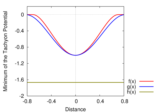
Figure 1: Plot of the minimum of tachyon potential versus distance. We have plotted $f(x)$= level $d^{2}$, $g(x)$= level 1/2 and $h(x)$= expected exact answer. We have used the unit $g^{2}=1/32$.

On plotting the minimum of the potential as a function of $d$ (see Fig. 1) we see that the dependence on the distance $d$ is less pronounced after inclusion of the level 1/2 field as compared to the case of the pure tachyon potential. We also see that the critical value $d_{c}$ of $d$ up to which the tachyon potential has a minimum is now given by the solution to the equation

$$1-2d_{c}^{2}+d_{c}^{2}\left(\frac{16}{27}\right)^{2d_{c}^{2}-1}\left(2^{\frac{3}{2}-d_{c}^{2}}+2^{-2d_{c}^{2}}\right)^{-1}=0\,.$$ (3.21)

This is larger than the original value $1/\sqrt{2}$ indicating that the after taking into account corrections due to higher level fields the minimum of the potential remains below zero for a larger range of $d$. We expect the dependence on $d$ to reduce as we include more and more fields into the analysis. The true minimum of the tachyon potential should not depend on what distance we separate out the branes initially. This has been shown schematically in Fig. 1 .

4 Rolling non-universal tachyon

In this section we shall set up the formalism for describing the rolling tachyon solution on a separated brane-antibrane pair. We begin by considering an unstable D-brane system in bosonic string theory, containing a primary boundary operator $V$ of dimension $h<1$. This would correspond to a tachyon of mass${}^{2}=(h-1)$ in the spectrum. Our goal will be to construct a time dependent solution in the theory that describes the rolling of this tachyon away from the maximum of its potential.

Let $X=-iX^{0}$ denote the world-sheet scalar associated with the Wick rotated time coordinate. Then the operator

$$\widetilde{V}=V\,e^{i\sqrt{1-h}X}\,,$$ (4.1)

is an operator of dimension 1. This will be an exactly marginal operator if a product of arbitrary number of these operators does not contain an operator of dimension 1. Since a product of $n$ of these operators contains a factor of $e^{in\sqrt{1-h}X}$ of dimension $n^{2}(1-h)$, we see that the condition for exact marginality is easily achieved if $n^{2}(1-h)>1$ for $n\geq 2$, ı.e. if

$$h<{3\over 4}\,.$$ (4.2)

Since

$$\widetilde{V}(u)\widetilde{V}(u^{\prime})=K(u-u^{\prime})^{2-4h}e^{2i\sqrt{1-h}X(u^{\prime})}+\cdots$$ (4.3)

with $K$ denoting a constant and $\cdots$ denoting less singular terms, we see that for $h$ satisfying (4.2) the power of $(u-u^{\prime})$ in $V(u)V(u^{\prime})$ is larger then $-1$.

Consider now deforming the theory by adding to the action the term

$$\lambda\,\int du\,\widetilde{V}(u)\,.$$ (4.4)

Then the correlation functions in the deformed theory are computed by inserting into the correlation function of the undeformed theory the operator

$$\exp\left[-\lambda\,\int du\,\widetilde{V}(u)\right]\,.$$ (4.5)

After expanding the exponential factor we encounter multiple integrals of the form

$$\int du_{1}\int du_{2}\cdots\int du_{n}\,\widetilde{V}(u_{1})\cdots\widetilde{V}(u_{n})\,.$$ (4.6)

Since the operator product $\widetilde{V}(u_{i})\widetilde{V}(u_{j})$ is less singular than $(u_{i}-u_{j})^{-1}$, the above integral, inserted into a correlation function of the undeformed theory, gives completely regular integrals. Thus the correlation functions of the deformed theory are determined in terms of the correlation functions of the undeformed theory without any need to regularize the theory.

The operator $\widetilde{V}$ defined in (4.1) is of course not hermitian and hence the deformation (4.5) does not produce a physical background of the open string theory. This problem disappears after inverse Wick rotation $X\to-iX^{0}$. In this case the operator $\widetilde{V}(u)$ becomes $V(u)\,e^{X^{0}(u)\sqrt{1-h^{2}}}$ and the deformed theory describes a physical open string background. This in fact describes the rolling of the tachyon associated with the operator $V$ away from its maximum.

Generalization to the case of unstable D-branes in superstring theory is straightforward. Suppose we have a vertex operator described by the superfield $V_{-1}+\theta V_{0}$ with $(V_{-1},V_{0})$ having dimensions $(h,h+{1\over 2})$ and $\theta$ denoting the fermionic world-sheet coordinate. If $V_{-1}$ is a superconformal primary then this describes a tachyon on the D-brane world-volume of mass${}^{2}=(h-{1\over 2})$. We now denote as before by $X=-iX^{0}$ the world-sheet scalar associated with the Wick rotated time coordinate, and by $\psi=-i\psi^{0}$ its fermionic superpartner. Then the vertex operator

$$\widetilde{V}(\theta)=e^{i\,(X+\theta\psi)\,\sqrt{{1\over 2}-h}}\left(V_{-1}+\theta V_{0}\right)\equiv(\widetilde{V}_{-1}+\theta\widetilde{V}_{0})\,$$ (4.7)

describes a primary superfield whose lowest component has dimension 1/2. Here

$$\widetilde{V}_{-1}=\widetilde{V}(\theta)|_{\theta=0}=e^{iX\sqrt{{1\over 2}-h}}\,V_{-1},\qquad\widetilde{V}_{0}=\int d\,\theta\,\widetilde{V}(\theta)=e^{iX\sqrt{{1\over 2}-h}}\left(V_{0}+i\psi V_{-1}\sqrt{{1\over 2}-h}\right)\,,$$ (4.8)

Hence the highest component $\widetilde{V}_{0}$ of the superfield $\widetilde{V}(\theta)$ is marginal. In order for it to be exactly marginal we need its operator product with itself not to contain any other marginal deformation. Repeating the analysis for bosonic string theory we see that this can be guaranteed if

$$h<{1\over 4}\,.$$ (4.9)

Furthermore in this case the operator product of (4.8) with itself has a singularity that is milder than $(u-u^{\prime})^{-1}$. Thus the correlation functions in the theory deformed by the operator

$$\lambda\,\int du\,\widetilde{V}_{0}(u)\,,$$ (4.10)

are unambiguously determined in terms of the correlation functions in the undeformed theory without any need to regularize the theory.

As in the case of bosonic string theory, the operator $\widetilde{V}_{0}$ defined in (4.8) is not hermitian and hence deformation (4.10) does not represent a physical open string background. However by the inverse Wick rotation $iX\to X^{0}$, $i\psi\to\psi^{0}$ we get a hermitian vertex operator

$$\widetilde{V}_{0}=e^{X^{0}\sqrt{{1\over 2}-h}}\left(V_{0}+\psi^{0}V_{-1}\sqrt{{1\over 2}-h}\right)\,.$$ (4.11)

Thus the deformation of the original theory by this operator produces a physical open string background.

We conclude this section with two examples. The first example is a D$p$-$\bar{\rm D}$$p$ brane wrapped on a circle of radius $R$. Let $y$ denote the coordinate along the compact circle and $Y$ and $\psi_{y}$ be the associated world-sheet scalar and fermion fields respectively. For $R>\sqrt{2}$ there is a tachyon of mass${}^{2}={1\over R^{2}}-{1\over 2}$ described by the vertex operator:

$$V_{-1}+\theta V_{0}=\sigma_{1}\,\cos\left({Y+\theta\psi_{y}\over R}\right)=\sigma_{1}\,\left(\cos{Y\over R}-{1\over R}\,\theta\,\psi_{y}\,\sin{Y\over R}\right)\,,$$ (4.12)

where the Pauli matrix $\sigma_{1}$ represents the external Chan-Paton factor. $V_{-1}$ has dimension $h=R^{-2}$. Thus (4.8), (4.9) shows that for

$$R>2\,$$ (4.13)

we can construct an exactly marginal deformation generated by the operator

$$\widetilde{V}_{0}=\sigma_{1}\,e^{iX\sqrt{{1\over 2}-{1\over R^{2}}}}\,\left(-\psi_{y}\,{1\over R}\,\sin{Y\over R}+i\psi\sqrt{{1\over 2}-{1\over R^{2}}}\,\cos{Y\over R}\right)\,.$$ (4.14)

The operator product $\widetilde{V}(u)\widetilde{V}(u^{\prime})$ is less singular than $(u-u^{\prime})^{-1}$ and hence the correlation functions of the deformed theory are free from any singularity.

The second example, which we shall analyze in detail in later sections, is a D$p$-$\bar{\rm D}p$ brane pair separated by a distance $2\pi d$ in the transverse direction. Let $y$ denote the transverse coordinate along the direction of separation of the branes, $\widetilde{Y}$ denote the world-sheet scalar dual to the scalar field $Y$ associated with the coordinate $y$, and $\widetilde{\psi}_{y}$ denote the fermionic superpartner of $\widetilde{Y}$. In this case for $d<{1\over\sqrt{2}}$ there is a tachyonic mode on this system, represented by the vertex operator

$$V_{-1}+\theta V_{0}=\sigma^{+}\,e^{i(\widetilde{Y}+\theta\widetilde{\psi}_{y})\,d}+\sigma^{-}\,e^{-i(\widetilde{Y}+\theta\widetilde{\psi}_{y})\,d}=\sigma^{+}\,(1+i\theta\widetilde{\psi}_{y}\,d)\,e^{i\widetilde{Y}\,d}+\sigma^{-}\,(1-i\theta\widetilde{\psi}_{y}\,d)\,e^{-i\widetilde{Y}\,d}\,,$$ (4.15)

where $\sigma^{\pm}$ are the external Chan-Paton factors

$$\sigma^{+}=\pmatrix{0&1\cr 0&0},\qquad\sigma^{-}=\pmatrix{0&0\cr 1&0}\,.$$ (4.16)

Since $V_{-1}$ has dimension $h=d^{2}$ we see from (4.8), (4.9) that for

$$d<{1\over 2}\,$$ (4.17)

we can construct an exactly marginal deformation generated by the operator

$$\widetilde{V}_{0}=i\,\sigma^{+}\,e^{iX\sqrt{{1\over 2}-{d^{2}}}}\,e^{i\widetilde{Y}\,d}\,\psi^{+}+i\,\sigma^{-}\,e^{iX\sqrt{{1\over 2}-{d^{2}}}}\,e^{-i\widetilde{Y}\,d}\,\psi^{-}$$ (4.18)

where

$$\psi^{+}=\left(\widetilde{\psi}_{y}\,d+\psi\sqrt{{1\over 2}-{d^{2}}}\right),\qquad\psi^{-}=\left(-\widetilde{\psi}_{y}\,d+\psi\sqrt{{1\over 2}-{d^{2}}}\right)\,.$$ (4.19)

Again the operator product $\widetilde{V}(u)\widetilde{V}(u^{\prime})$ is less singular than $(u-u^{\prime})^{-1}$ and hence the correlation functions of the deformed theory are free from any singularity.

5 Time dependence of pressure on a separated brane-antibrane system with a rolling tachyon

We consider a brane-antibrane system separated by a distance $2\pi d$ with $d<{1\over 2}$ in the presence of a rolling tachyon background generated by the deformation

$$\lambda\int du\,\widetilde{V}_{0}(u)\,,$$ (5.1)

with $\widetilde{V}_{0}$ given in (4.18). Let $p(x)$ denotes the $x$-dependent tangential pressure of the brane generated by this deformation and $p_{0}$ be the pressure in the absence of this deformation. $p(x)/p_{0}$ has a Fourier expansion of the form

$$p(x)/p_{0}=\sum_{n\geq 0}a_{n}e^{inx\sqrt{{1\over 2}-{d^{2}}}}\,,$$ (5.2)

for constants $a_{n}$. The coefficients $a_{n}$ can be found by examining the boundary state of the deformed brane if it is known, or equivalently from the disk one point function of the matter vertex operator $e^{-inX\sqrt{{1\over 2}-{d^{2}}}}$ inserted at the center of the unit disk in the deformed theory:

$$a_{n}=\langle e^{-inX(0)\sqrt{{1\over 2}-{d^{2}}}}\rangle_{deformed}\,,$$ (5.3)

where $\langle~{}\rangle_{deformed}$ denotes the correlation function in the deformed theory, normalized such that in the undeformed theory the disk partition function is 1. Representing the deformation of the Euclidean world-sheet action as

$$\lambda\,\int du\widetilde{V}_{0}(u)\,,$$ (5.4)

with $u$ labeling the coordinates on the boundary of the disk, we can reexpress $a_{n}$ as[33]

$$a_{n}={1\over 2}\sum_{r=0}^{\infty}{\lambda^{2r}\over(2r)!}\,\int du_{1}\cdots du_{2r}\,\left\langle e^{-inX(0)\sqrt{{1\over 2}-{d^{2}}}}Tr\left(\widetilde{V}_{0}(u_{1})\cdots\widetilde{V}_{0}(u_{2r})\right)\right\rangle_{0}\,,$$ (5.5)

where $\langle~{}\rangle_{0}$ denotes the correlation function in the undeformed theory on the unit disk and $Tr$ denotes trace over the Chan-Paton factors. In (5.5) we have used the fact that the trace over the Chan-Paton factor vanishes if we have odd number of $\widetilde{V}_{0}$ insertions on the boundary. The overall factor of $1/2$ is a reflection of the factor of 2 appearing in the expression for the unperturbed pressure $p_{0}$ from the trace over the Chan-Paton factors. Using the results

$$\left(\sigma^{+}\right)^{2}=\left(\sigma^{-}\right)^{2}=0\,,$$ (5.6)

we see that only two strings of Chan-Paton factors contribute to the correlation function – $Tr(\sigma^{+}\sigma^{-}\sigma^{+}\sigma^{-}\cdots)$ and $Tr(\sigma^{-}\sigma^{+}\sigma^{-}\sigma^{+}\cdots)$. The associated vertex operators must be cyclically ordered on the boundary of the unit disk. Both strings give the same contribution. Finally $X$-momentum conservation, together with the fact that each of the $\widetilde{V}_{0}$ carries $X$-momentum $\sqrt{{1\over 2}-{d^{2}}}$, shows that the correlator (5.5) is non-vanishing only when $n=2r$. Using this we can express (5.5) as

$$\displaystyle a_{2r+1} = 0\quad\hbox{for $r\in{\hbox{ Z\kern-4.55244ptZ}}$}$$

$$a_{2r} = \lambda^{2r}\,\int_{0}^{2\pi}\,dt_{1}\int_{0}^{t_{1}}\,dt_{2}\cdots\int_{0}^{t_{2r-1}}\,dt_{2r}$$ (5.7)

$$\Bigg{\langle}e^{-2irX(0)\sqrt{{1\over 2}-{d^{2}}}}\,e^{iX(u_{1})\sqrt{{1\over 2}-{d^{2}}}}\cdots e^{iX(u_{2r})\sqrt{{1\over 2}-{d^{2}}}}$$

$$\times\,e^{i\widetilde{Y}(u_{1})\,d}\,e^{-i\widetilde{Y}(u_{2})\,d}\cdots e^{i\widetilde{Y}(u_{2r-1})\,d}e^{-i\widetilde{Y}(u_{2r})\,d}$$

$$\times\,(i)^{2r}\,\psi^{+}(u_{1})\psi^{-}(u_{2})\psi^{+}(u_{3})\psi^{-}(u_{4})\cdots\psi^{+}(u_{2r-1})\psi^{-}(u_{2r})\Bigg{\rangle}\,,\qquad u_{i}\equiv e^{it_{i}}\,,$$

$$\quad\hbox{for $r\in{\hbox{ Z\kern-4.55244ptZ}}$, $r\geq 0$}\,.$$

Note that we have replaced $\int\prod du_{i}$ by $\int\prod_{i}dt_{i}$, – this requires that in computing the correlators on the right hand side of (5) all the fields need to be defined in the $t$-coordinate system. The part of the correlator involving the scalar fields $X$ and $\widetilde{Y}$ gives

$$\prod_{i<j}|u_{i}-u_{j}|^{1-2{d^{2}}+2(-1)^{i+j}{d^{2}}}=\prod_{i<j}\left|2\sin{t_{i}-t_{j}\over 2}\right|^{1-2{d^{2}}+2(-1)^{i+j}{d^{2}}}\,.$$ (5.8)

On the other hand the fermionic correlators can be calculated with the help of Wick’s theorem using the two point functions

$$\langle\psi^{+}(u_{1})\psi^{+}(u_{2})\rangle=\langle\psi^{-}(u_{1})\psi^{-}(u_{2})\rangle={i\over 2}\,{e^{i(t_{i}+t_{j})/2}\over u_{1}-u_{2}}={1\over 2}{1\over 2\sin{t_{i}-t_{j}\over 2}},$$

$$\langle\psi^{+}(u_{1})\psi^{-}(u_{2})\rangle=i\,\left({1\over 2}-2\,d^{2}\right)\,{e^{i(t_{i}+t_{j})/2}\over u_{1}-u_{2}}=\left({1\over 2}-2\,d^{2}\right)\,{1\over 2\sin{t_{i}-t_{j}\over 2}}\,.$$ (5.9)

Although the fermionic correlator in eq.(5) contains many terms we can organize them in a compact form by collecting all terms in which a certain number (say $s$) of $\psi^{+}$ pairs have been contracted with each other, an equal number of $\psi^{-}$ pairs have been contracted with each other, and the $(r-2s)$ left-over $\psi^{+}$’s have been contracted with $(r-2s)$ left-over $\psi^{-}$’s. After taking into account the combinatoric factors we can express (5) as

$$\displaystyle a_{2r} = \,(-1)^{r}\,\lambda^{2r}\,\int_{0}^{2\pi}\,dt_{1}\int_{0}^{t_{1}}\,dt_{2}\cdots\int_{0}^{t_{2r-1}}\,dt_{2r}\,\prod_{i<j}\left|2\sin{t_{i}-t_{j}\over 2}\right|^{1-2{d^{2}}+2(-1)^{i+j}{d^{2}}}$$

$$\sum_{s=0}^{[r/2]}{(1-4d^{2})^{r-2s}(-1)^{s}\over(r-2s)!(s!)^{2}2^{2s}2^{r}}\,\Bigg{[}\prod_{l=2s}^{r-1}\left(2\sin{t_{2l+1}-t_{2l+2}\over 2}\right)^{-1}$$

$$\prod_{k=0}^{s-1}\left\{\left(2\sin{t_{4k+1}-t_{4k+3}\over 2}\right)^{-1}\left(2\sin{t_{4k+2}-t_{4k+4}\over 2}\right)^{-1}\right\}$$

$$+(-1)^{P+P^{\prime}}\times\hbox{permutations $P$ of $t_{1},t_{3},\cdots t_{2r-1}$}\times\hbox{permutations $P^{\prime}$ of $t_{2},t_{4},\cdots t_{2r}$}\Bigg{]}\,,$$

where $[r/2]$ denotes the integral part of $r/2$.

Another compact representation of the correlators is provided by the superfield representation[33]. If we denote by $\widetilde{V}_{\pm}(u,\theta)$ the superfields

$$V_{\pm}(u,\theta)=e^{i(X+\theta\psi)\sqrt{{1\over 2}-d^{2}}}\,e^{\pm i(\widetilde{Y}+\theta\widetilde{\psi}_{y})\,d}\,,$$ (5.11)

then the expression for $a_{2r}$ given in (5) can be written as

$$\displaystyle a_{2r} = \lambda^{2r}\,\int_{0}^{2\pi}\,dt_{1}\int_{0}^{t_{1}}\,dt_{2}\cdots\int_{0}^{t_{2r-1}}\,dt_{2r}\int d\theta_{1}\cdots\int d\theta_{2r}$$ (5.12)

$$\left\langle e^{-2irX(0)}\,\widetilde{V}^{+}(u_{1},\theta_{1})\widetilde{V}^{-}(u_{2},\theta_{2})\widetilde{V}^{+}(u_{3},\theta_{3})\widetilde{V}^{-}(u_{4},\theta_{4})\cdots\widetilde{V}^{+}(u_{2r-1},\theta_{2r-1})\widetilde{V}^{-}(u_{2r},\theta_{2r})\right\rangle$$

$$= \lambda^{2r}\,\int_{0}^{2\pi}\,dt_{1}\int_{0}^{t_{1}}\,dt_{2}\cdots\int_{0}^{t_{2r-1}}\,dt_{2r}\int d\theta_{1}\cdots\int d\theta_{2r}$$

$$\qquad\qquad\prod_{i<j}\left[2\sin{t_{i}-t_{j}\over 2}+\theta_{i}\theta_{j}\right]^{1-2{d^{2}}+2(-1)^{i+j}{d^{2}}}\,.$$

After integration over $\theta_{i}$ eq.(5.12) reduces to (5).

Once the coefficients $a_{n}$ have been calculated, we can use (5.2) to calculate $p(x)$. In fact after the inverse Wick rotation $ix\to x^{0}$ we get

$$p(x)/p_{0}=\sum_{r\geq 0}a_{2r}e^{2rx^{0}\sqrt{{1\over 2}-d^{2}}}\,.$$ (5.13)

Since $a_{2r}\propto\lambda^{2r}$, we can absorb $\lambda$ into an additive constant in $x^{0}$. Thus by suitable choice of the origin of the $x^{0}$ coordinate we can set $\lambda=(\sqrt{2}\pi)^{-1}$. In this case (5) reduces to

$$\displaystyle a_{2r} = \,(-1)^{r}\,\int_{0}^{2\pi}\,{dt_{1}\over 2\pi}\int_{0}^{t_{1}}\,{dt_{2}\over 2\pi}\cdots\int_{0}^{t_{2r-1}}\,{dt_{2r}\over 2\pi}\,\prod_{i<j}\left|2\sin{t_{i}-t_{j}\over 2}\right|^{1-2{d^{2}}+2(-1)^{i+j}{d^{2}}}$$

$$\sum_{s=0}^{[r/2]}{(1-4d^{2})^{r-2s}\,(-1)^{s}\,\over(r-2s)!(s!)^{2}2^{2s}}\,\Bigg{[}\prod_{l=2s}^{r-1}\left(2\sin{t_{2l+1}-t_{2l+2}\over 2}\right)^{-1}$$

$$\prod_{k=0}^{s-1}\left\{\left(2\sin{t_{4k+1}-t_{4k+3}\over 2}\right)^{-1}\left(2\sin{t_{4k+2}-t_{4k+4}\over 2}\right)^{-1}\right\}$$

$$+(-1)^{P+P^{\prime}}\times\hbox{permutations $P$ of $t_{1},t_{3},\cdots t_{2r-1}$}\times\hbox{permutations $P^{\prime}$ of $t_{2},t_{4},\cdots t_{2r}$}\Bigg{]}\,.$$

6 Numerical results

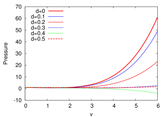
Figure 2: Plot of the pressure as a function of $v=e^{2\sqrt{{1\over 2}-d^{2}}x^{0}}$ for various values of $d$.

We have evaluated the first few coefficients given in (5) using Monte Carlo integration techniques. The results are given in table 1. The integrand is generated using a code in Mathematica and then we use VEGAS[34] to do the multidimensional integrals. Since these give the first few terms in the expansion of $p(x^{0})/p_{0}$ in a power series in $v\equiv e^{2x^{0}\sqrt{{1\over 2}-d^{2}}}$, we cannot reliably estimate the late time behaviour of $p(x^{0})$ using these results. A plot of pressure as a function of $v\equiv e^{2x^{0}\sqrt{{1\over 2}-d^{2}}}$ is shown in Fig. 2. From this it seems that the function does not display the wild oscillation of the kind seen in the tachyon profile computation associated with the rolling tachyon solution in string field theory; instead it may have a finite radius of convergence, and may admit an analytic continuation to infinite time as in the case of the behaviour of the pressure in the $d=0$ case. With our present data it is not possible to make any reliable estimate of the asymptotic value of the pressure. Nevertheless we give in table 2 the results of fitting a ratio of quadratic functions of $v$ to the series expansion. For the $d=0$ case the exact answer is known and it agrees with the result given in the table. If we take these results seriously then within numerical errors these results are consistent with the hypothesis that at late time the pressure vanishes.

	r=0	r=1	r=2	r=3	r=4
d=0	1	0.4999999 (1.5E-07)	0.2500775 (3.5E-05)	0.1249626 (2.3E-05)	0.06246 (1.0E-04)
d=0.1	1	0.4803255 (1.6E-07)	0.2284956 (3.2E-05)	0.1079812 (2.0E-05)	0.05088 (1.8E-05)
d=0.2	1	0.4250437 (1.8E-07)	0.1719809 (2.4E-05)	0.0671200 (1.4E-05)	0.02550 (1.3E-05)
d=0.3	1	0.3442298 (3.5E-07)	0.1003526 (1.8E-05)	0.0243640 (9.6E-05)	0.00413 (2.2E-05)
d=0.4	1	0.2512369 (1.0E-05)	0.0338092 (5.0E-05)	-0.0039147 (2.9E-05)	-0.00429 (2.8E-05)
d=0.5	1	0	-0.0416668 (1.5E-07)	0	0.001729 (1.2 E-05)

Table 1: The table containing the coefficients $(-1)^{r}a_{2r}$ calculated from (5). The numbers in the parenthesis are the estimated errors of the numerical calculations.

Separation	(2,2) Pade Approximation	Late Time Pressure
d=0	$\{1+2kv\}/\{1+(1/2+2k)v+kv^{2}\}$	0
d=0.1	$\{1+(0.20032)v+(0.00052)v^{2}\}/\{1+(0.68065)v+(0.09895)v^{2}\}$	0.00526
d=0.2	$\{1+(0.23555)v+(0.00067)v^{2}\}/\{1+(0.6606)v+(0.10945)v^{2}\}$	0.00612
d=0.3	$\{1+(0.27651)v-(0.00325)v^{2}\}/\{1+(0.6207)v+(0.11007)v^{2}\}$	-0.02936
d=0.4	$\{1+(0.19569)v-(0.00283)v^{2}\}/\{1+(0.4469)v+(0.07565)v^{2}\}$	-0.03741
d=0.5	$\{1-(0.000177)v^{2}\}/\{1+(0.04149)v^{2}\}$	-0.00427

Table 2: The table containing the Pade approximant results for the function representing $p(x^{0})/p_{0}$. Here $v\equiv e^{2x^{0}\sqrt{{1\over 2}-d^{2}}}$. The last column gives the late time behaviour of the pressure if we take these expressions seriously. In the first row $k$ is an arbitrary constant.

7 Discussion

We have seen in §5 that given a tachyon with mass² less than a certain critical value we can generate a deformation of the original CFT by an exactly marginal operator describing a rolling tachyon solution. Furthermore the deformed theory does not require any additional renormalization beyond those required to renormalize the original CFT.

It turns out that precisely for these ranges of tachyon mass² we can generate a rolling tachyon solution of open string field theory following the method of [35, 36, 37, 38, 39, 40, 41, 42, 43, 46]. Let us first consider the case of open bosonic string theory. In this case if we have a matter sector vertex operator $\widetilde{V}$ of dimension 1, then we can generate a non-singular solution of open bosonic string field theory provided integrals of the form $\int du^{\prime}\widetilde{V}(u)\widetilde{V}(u^{\prime})$ do not diverge in the region $u^{\prime}\simeq u$[35, 36]. But this is precisely the condition that $\widetilde{V}(u)\widetilde{V}(u^{\prime})$ will have a singularity softer than $(u-u^{\prime})^{-1}$. Similarly the condition under which one can generate a non-singular solution in open superstring field theory corresponding to a dimension half matter vertex operator $\widetilde{V}_{-1}$ and its dimension 1 superpartner $\widetilde{V}_{0}$ is that $\int du^{\prime}\widetilde{V}_{-1}(u)\widetilde{V}_{0}(u^{\prime})$ and $\int du^{\prime}\widetilde{V}_{0}(u)\widetilde{V}_{0}(u^{\prime})$ do not diverge from $u^{\prime}\simeq u$ region[37, 38, 40]. For $\widetilde{V}_{-1}$ and $\widetilde{V}_{0}$ given in eq.(4.8) this happens precisely for $h<{1\over 4}$, ı.e. when (4.9) is satisfied. Thus both for bosonic and superstring field theory we can construct a non-singular solution describing a rolling non-universal tachyon when the boundary CFT associated with the solution can be defined without any need to regularize and renormalize the theory. It may be of interest to study these solutions numerically.

Acknowledgements: We would like to thank T. Erler for useful discussions and Girish Kulkarni and especially V. Ravindran for help in the numerical part of the work.

References

• [1] A. Sen, “Descent relations among bosonic D-branes,” Int. J. Mod. Phys.  A 14, 4061 (1999) [arXiv:hep-th/9902105].
• [2] A. Sen, “Universality of the tachyon potential,” JHEP 9912, 027 (1999) [arXiv:hep-th/9911116].
• [3] A. Sen and B. Zwiebach, “Tachyon condensation in string field theory,” JHEP 0003, 002 (2000) [arXiv:hep-th/9912249].
• [4] N. Moeller and W. Taylor, “Level truncation and the tachyon in open bosonic string field theory,” Nucl. Phys.  B 583, 105 (2000) [arXiv:hep-th/0002237].
• [5] D. Gaiotto and L. Rastelli, “Experimental string field theory,” JHEP 0308, 048 (2003) [arXiv:hep-th/0211012].
• [6] M. Schnabl, “Analytic solution for tachyon condensation in open string field theory,” Adv. Theor. Math. Phys.  10, 433 (2006) [arXiv:hep-th/0511286].
• [7] Y. Okawa, “Comments on Schnabl’s analytic solution for tachyon condensation in Witten’s open string field theory,” JHEP 0604, 055 (2006) [arXiv:hep-th/0603159].
• [8] E. Fuchs and M. Kroyter, “On the validity of the solution of string field theory,” JHEP 0605, 006 (2006) [arXiv:hep-th/0603195].
• [9] E. Fuchs and M. Kroyter, “Schnabl’s L(0) operator in the continuous basis,” JHEP 0610, 067 (2006) [arXiv:hep-th/0605254].
• [10] L. Rastelli and B. Zwiebach, “Solving open string field theory with special projectors,” arXiv:hep-th/0606131.
• [11] I. Ellwood and M. Schnabl, “Proof of vanishing cohomology at the tachyon vacuum,” JHEP 0702, 096 (2007) [arXiv:hep-th/0606142].
• [12] E. Fuchs and M. Kroyter, “Universal regularization for string field theory,” JHEP 0702, 038 (2007) [arXiv:hep-th/0610298].
• [13] Y. Okawa, L. Rastelli and B. Zwiebach, “Analytic solutions for tachyon condensation with general projectors,” arXiv:hep-th/0611110.
• [14] T. Erler, “Split string formalism and the closed string vacuum,” JHEP 0705, 083 (2007) [arXiv:hep-th/0611200].
• [15] T. Erler, “Split string formalism and the closed string vacuum. II,” JHEP 0705, 084 (2007) [arXiv:hep-th/0612050].
• [16] O. K. Kwon, B. H. Lee, C. Park and S. J. Sin, “Fluctuations around the Tachyon Vacuum in Open String Field Theory,” arXiv:0709.2888 [hep-th].
• [17] T. Takahashi, “Level truncation analysis of exact solutions in open string field theory,” arXiv:0710.5358 [hep-th].
• [18] A. Sen, “Rolling tachyon,” JHEP 0204, 048 (2002) [arXiv:hep-th/0203211].
• [19] A. Sen, “Tachyon condensation on the brane antibrane system,” JHEP 9808, 012 (1998) [arXiv:hep-th/9805170].
• [20] N. Berkovits, “The tachyon potential in open Neveu-Schwarz string field theory,” JHEP 0004, 022 (2000) [arXiv:hep-th/0001084].
• [21] N. Berkovits, A. Sen and B. Zwiebach, “Tachyon condensation in superstring field theory,” Nucl. Phys.  B 587, 147 (2000) [arXiv:hep-th/0002211].
• [22] P. J. De Smet and J. Raeymaekers, “Level four approximation to the tachyon potential in superstring field theory,” JHEP 0005, 051 (2000) [arXiv:hep-th/0003220].
• [23] A. Iqbal and A. Naqvi, “Tachyon condensation on a non-BPS D-brane,” arXiv:hep-th/0004015.
• [24] T. Erler, “Tachyon Vacuum in Cubic Superstring Field Theory,” arXiv:0707.4591 [hep-th].
• [25] A. Sen, “Tachyon matter,” JHEP 0207, 065 (2002) [arXiv:hep-th/0203265].
• [26] G. R. Dvali and S. H. H. Tye, “Brane inflation,” Phys. Lett.  B 450, 72 (1999) [arXiv:hep-ph/9812483].
• [27] N. Berkovits, “SuperPoincare invariant superstring field theory,” Nucl. Phys.  B 450, 90 (1995) [Erratum-ibid.  B 459, 439 (1996)] [arXiv:hep-th/9503099].
• [28] N. Berkovits, “A new approach to superstring field theory,” Fortsch. Phys.  48, 31 (2000) [arXiv:hep-th/9912121].
• [29] N. D. Lambert, H. Liu and J. M. Maldacena, “Closed strings from decaying D-branes,” JHEP 0703, 014 (2007) [arXiv:hep-th/0303139].
• [30] A. Sen, “Tachyon dynamics in open string theory,” Int. J. Mod. Phys.  A 20, 5513 (2005) [arXiv:hep-th/0410103].
• [31] D. Friedan, E. J. Martinec and S. H. Shenker, “Conformal Invariance, Supersymmetry And String Theory,” Nucl. Phys.  B 271, 93 (1986).
• [32] A. Sen, “Time evolution in open string theory,” JHEP 0210, 003 (2002) [arXiv:hep-th/0207105].
• [33] F. Larsen, A. Naqvi and S. Terashima, “Rolling tachyons and decaying branes,” JHEP 0302, 039 (2003) [arXiv:hep-th/0212248].
• [34] G. P. Lepage, “A New Algorithm For Adaptive Multidimensional Integration,” J. Comput. Phys.  27, 192 (1978).
• [35] M. Schnabl, “Comments on marginal deformations in open string field theory,” Phys. Lett.  B 654, 194 (2007) [arXiv:hep-th/0701248].
• [36] M. Kiermaier, Y. Okawa, L. Rastelli and B. Zwiebach, “Analytic solutions for marginal deformations in open string field theory,” arXiv:hep-th/0701249.
• [37] T. Erler, “Marginal Solutions for the Superstring,” JHEP 0707, 050 (2007) [arXiv:0704.0930 [hep-th]].
• [38] Y. Okawa, “Analytic solutions for marginal deformations in open superstring field theory,” JHEP 0709, 084 (2007) [arXiv:0704.0936 [hep-th]].
• [39] E. Fuchs, M. Kroyter and R. Potting, “Marginal deformations in string field theory,” JHEP 0709, 101 (2007) [arXiv:0704.2222 [hep-th]].
• [40] Y. Okawa, “Real analytic solutions for marginal deformations in open superstring field theory,” JHEP 0709, 082 (2007) [arXiv:0704.3612 [hep-th]].
• [41] I. Ellwood, “Rolling to the tachyon vacuum in string field theory,” arXiv:0705.0013 [hep-th].
• [42] E. Fuchs and M. Kroyter, “Marginal deformation for the photon in superstring field theory,” JHEP 0711, 005 (2007) [arXiv:0706.0717 [hep-th]].
• [43] B. H. Lee, C. Park and D. D. Tolla, “Marginal Deformations as Lower Dimensional D-brane Solutions in Open String Field theory,” arXiv:0710.1342 [hep-th].
• [44] M. Kiermaier and Y. Okawa, “Exact marginality in open string field theory: a general framework,” arXiv:0707.4472 [hep-th].
• [45] M. Kiermaier and Y. Okawa, “General marginal deformations in open superstring field theory,” arXiv:0708.3394 [hep-th].
• [46] O. K. Kwon, “Marginally Deformed Rolling Tachyon around the Tachyon Vacuum in Open String Field Theory,” arXiv:0801.0573 [hep-th].