Probing the Binary Black Hole Merger Regime with Scalar Perturbations

Abstract

We present results obtained by scattering a scalar field off the curved background of a coalescing binary black hole system. A massless scalar field is evolved on a set of fixed backgrounds, each provided by a spatial hypersurface generated numerically during a binary black hole merger. We show that the scalar field scattered from the merger region exhibits quasinormal ringing once a common apparent horizon surrounds the two black holes. This occurs earlier than the onset of the perturbative regime as measured by the start of the quasinormal ringing in the gravitational waveforms. We also use the scalar quasinormal frequencies to associate a mass and a spin with each hypersurface, and observe the compatibility of this measure with the horizon mass and spin computed from the dynamical horizon framework.

I Introduction

Over the past thirty years, numerical evolutions of binary black hole (BBH) systems have provided deeper and deeper insight into the properties of the vacuum two-body problem of general relativity. Today a number of codes Pretorius (2005); Campanelli et al. (2006); Baker et al. (2006a); Herrmann et al. (2007); Gonzalez et al. (2007); Koppitz et al. (2007); Pfeiffer et al. (2007); Tichy and Marronetti (2007) are able to accurately evolve black hole binaries; in particular, the merger regime itself is now available for studies. It was shown in reference Buonanno et al. (2007); Berti et al. (2007a) that the merged system seems to enter the perturbative stage while it is still evolving and radiating energy and angular momentum. This is in agreement with earlier results from the Close Limit approximation Price and Pullin (1994) and from the Lazarus project Baker et al. (2002).

In order to study the transition between the nonlinear merger stage and the final ringing black hole, we scatter a test scalar field off the geometry generated in the inspiral and merger of the binary system. Test fields and perturbation theory have traditionally been used to study excitations on a single stationary black hole spacetime, both for the Schwarzschild Regge and Wheeler (1957); Zerilli (1970); Vishveshwara (1970) and for the Kerr solutions Teukolsky (1973). Numerical methods were used in several scenarios (see for instance Krivan et al. (1996) and Dorband et al. (2006)); more recently, these results have been extended to more general black hole solutions, including non-vacuum spacetimes Shao et al. (2005) and models with non-flat asymptotic topology Molina et al. (2004); Chan and Mann (1997).

An interesting result of quasinormal mode (QNM) evolution on non-stationary, spherically symmetric black hole spacetimes is that the mass extracted from the complex quasinormal frequency tracks the time-dependent black hole (BH) mass quite closely (modulo a delay effect), equaling the constant quasinormal frequency one would obtain on a static spacetime with the mass parameter equal to the instantaneous mass at each time Shao et al. (2005). This adiabatic picture has an intriguing parallel in black hole thermodynamics: the application of the first law to a spacetime containing an axisymmetric dynamical horizon shows that the mass increase between two cross sections with horizon area $A_{1}$ and $A_{2}$ and angular momentum $J_{1}$ and $J_{2}$ is given exactly by $M(A_{2},J_{2})-M(A_{1},J_{1})$, where $M(A,J)$ represents the functional dependence of the mass $M$ on $A$ and $J$ for a Kerr solution Ashtekar (2003). In other words, as far as the first law of thermodynamics is concerned, this portion of the spacetime can formally be pictured as a stack of spatial hypersurfaces, with each slice belonging to a member of the Kerr family with a different mass and spin parameter.

In this study we aim to address some questions concerning the transition between a system of two inspiraling black holes and a single perturbed black hole. We investigate how early during the BBH evolution the scalar field probe exhibits the quasinormal ringing phase ordinarily expected from a spacetime containing a single black hole, and what features this phase displays when compared to gravitational wave quasinormal ringing of the single stationary black hole that is left behind by the coalescence process. Based on these considerations we present a novel strategy that consists of (i) simulating a BBH merger and extracting horizon information from the merged black hole, (ii) taking snapshots of the spatial geometry obtained in the BBH merger at a sequence of coordinate times, (iii) evolving a massless scalar field on the corresponding spatial hypersurfaces, and (iv) observing the scalar field undergo a quasinormal ringing phase and extracting its complex frequency, which in turn can be converted into a mass and a spin parameter using the functional dependence of the quasinormal frequencies on these two parameters prescribed by perturbation theory. We then compare these estimates to the mass and spin extracted directly from the horizon.

This method has the benefit of effectively separating the evolution time of the binary system from the relaxation time of the scalar perturbations, allowing for a measure of the “instantaneous” properties of the foliation. Notice that this procedure is effectively equivalent to the evolution of a scalar field on the fictitious spacetime one would obtain by selecting each spatial surface and freezing it in time. This of course is not meant to constitute a physical solution to the coupled scalar-gravitational system: as emphasized above the scalar field is used here exclusively as a probing agent for individual hypersurfaces.

We will present a brief overview of scalar perturbations in section II, along with the method we use to evolve the scalar wave equation on a numerically-generated curved background, extract the complex frequencies and associate a mass and spin parameter to them. Section III contains the results of our scalar field evolutions, along with the corresponding waveforms and analysis of errors. Finally, in our concluding section IV, we will discuss the results.

II Scalar field evolution

The behavior of a massless scalar field on the background of a single Kerr black hole has been the subject of extensive analytical treatments. A good introduction is given in reference Chandrasekhar (1985) and a thorough treatment of the subject can be found in Nollert’s Nollert (1999) and Kokkotas and Schmidt’s review works Kokkotas and Schmidt (1999).

II.1 Quasinormal ringing

The behavior of a massless scalar field $\Phi$ on the background provided by a Kerr black hole of mass $M$ and Kerr spin parameter $a=J/M$ is governed by the source-free scalar wave equation:

$$\square\Phi:=g_{ab}\nabla^{a}\nabla^{b}\Phi=0\,.$$ (1)

Separating out the angular variables, one reaches a wave equation with a potential Teukolsky (1973). Upon further study, one finds that the field exhibits many of the well-known features of waves impinging on a potential; for instance, it exhibits quasinormal ringing, i.e. a phase of decaying oscillations characterized by a certain complex frequency spectrum.

The complex nature of the frequency spectrum leads to several undesirable consequences, some of which have direct ramifications on our ability to detect and characterize quasinormal ringing in a numerical simulation: first and foremost, the spectrum of quasinormal modes does not constitute a complete set of eigenfunctions Nollert (1999); Ching et al. (1996); Chandrasekhar (1985): early on, the behavior of the scalar field depends on the process that generated the perturbation, and the field is said to undergo the prompt response regime, where $\Phi$ still displays memory of the perturbing mechanism Ching et al. (1998). Additionally, at late times the backscattering off the curvature will overtake the by-now feeble damped oscillations and dominate the waveforms, generating the so-called tails Ching et al. (1998). A Green’s-function analysis of the origin of these three phases, along with a convergence study of the quasinormal mode expansion is presented in Leaver (1986) for Schwarzschild and in Berti and Cardoso (2006) for Kerr black holes. The question then arises about how to identify the onset time of quasinormal ringing, since an accurate determination of this quantity is of the utmost importance while fitting for the quasinormal frequencies. This issue is usually referred to as the time shift problem; for a discussion of its influence on the bias of the fitted parameters, see Dorband et al. (2006). Also, concepts such as the fraction of a given waveform that can be identified as each quasinormal mode and the gravitational energy contained in each quasinormal mode cannot be defined in rigorous terms Nollert and Price (1999); the absence of such auxiliary notions also poses serious complications to identifying the onset of quasinormal ringing in a numerical waveform, and quantifying its quasinormal content. Berti et al. Berti et al. (2007a) review this issue from the numerical point of view.

Notice that, due to their dependence on the mass $M$ and spin parameter $j=a/M$ of the background Kerr solution, the quasinormal ringing portion of the scattered waves carries information about $M$ and $j$ away from the scattering center (a property which, for instance, makes gravitational quasinormal ringing a powerful tool for gravitational wave astronomy Berti et al. (2006a)).

In this work, we use scalar perturbations to probe the parameters describing the final black hole that results from the binary coalescence. In order to provide as accurate a depiction of the black hole as possible, we will first have to devise a strategy to tackle the ambiguities associated with quasinormal modes and find a reliable strategy to detect and measure the quasinormal components in a waveform. In section II.5 we will present our experimental method.

II.2 Scalar field evolution on a numerically generated background

We evolve a scalar field on a numerically generated background obtained from a binary black hole evolution. We take snapshots of the spatial geometry and then use each of these as a time-independent background on which the scalar field propagates.

During the course of the evolution, we store the values of the grid functions corresponding to the gravitational variables at a sequence of coordinate times $\left\{t_{N}\right\}$, which we denote with a bar:

$$\bar{\gamma}_{ij}(x^{k})\equiv\gamma_{ij}(t_{N},x^{k})$$ (2)

$$\bar{K}_{ij}(x^{k})\equiv K_{ij}(t_{N},x^{k})$$ (3)

$$\bar{\alpha}(x^{k})\equiv\alpha(t_{N},x^{k})$$ (4)

$$\bar{\beta}^{i}(x^{k})\equiv\beta^{i}(t_{N},x^{k})$$ (5)

and evolve a scalar field on the background provided by the corresponding frozen geometry. In this sense, $\Phi$ is nothing more than a probing agent for each of the spatial slices on which we perform the experiment, and is meant solely to provide information, through its scattering, about the curvature of each single slice rather than to explore a scalar-gravitational coupling of an actual physical system.

II.3 Background spacetime

The evolution of the gravitational variables $\gamma_{ij}$ and $K_{ij}$ is performed according to the BSSN system Nakamura et al. (1987); Shibata and Nakamura (1995); Baumgarte and Shapiro (1999), as implemented in the PSU code through the Kranc generator Husa et al. (2006). The fourth order finite differencing code is based on the Cactus infrastructure cac and is endowed with Carpet’s mesh refinement capabilities Schnetter et al. (2004). The gauge variables $\alpha$ and $\beta^{i}$ are initialized and evolved according to the moving puncture prescription Campanelli et al. (2006); Baker et al. (2006a), while the initial data are generated following Ansorg et al. (2004).

For the binary coalescence runs, we choose an initial configuration usually referred to as R1 Baker et al. (2006b): this setup represents two non-spinning black holes with irreducible masses equal to $0.505\mathcal{M}$ (where $\mathcal{M}$ denotes a mass scale related to the ADM mass via $E_{\mathrm{ADM}}/\mathcal{M}=0.9957$). The two black holes start at a coordinate separation of $6.514\mathcal{M}$, with linear momenta perpendicular to the separation vector and equal to $0.133\mathcal{M}$. Further details regarding our code and our earlier study of this system can be found in Vaishnav et al. (2007). We used a reference spatial resolution of $\mathcal{M}/51.2$, and evolved some simulations at two extra resolutions ($\mathcal{M}/44.8$ and $\mathcal{M}/57.6$) to obtain an estimate for the truncation errors (see section III.3 below).

Figure 1 plots the gravitational wave from the simulated system: the two black holes inspiral around each other for about two orbits before plunging and forming a single final perturbed black hole whose parameters can be inferred, due to energy and angular momentum conservation, from the emitted radiation in terms of the Newman-Penrose scalar $\Psi_{4}$, as discussed in Campanelli and Lousto (1999). For the $\mathcal{M}/51.2$ resolution run, starting with an initial ADM mass and angular momentum equal to $E_{\mathrm{ADM}}/\mathcal{M}=0.9957$ and $J_{\mathrm{ADM}}/\mathcal{M}^{2}=0.862$, the system radiates $E_{\mathrm{rad}}/\mathcal{M}=0.032\pm 0.005$ and $J_{\mathrm{rad}}/\mathcal{M}^{2}=0.22\pm 0.01$, leaving behind a final black hole with $E_{f}/\mathcal{M}=0.963\pm 0.005$ and $J_{f}/\mathcal{M}^{2}=0.64\pm 0.01$, in agreement with the estimates of mass and spin provided by the analysis of the fundamental quasinormal tone of $\Psi_{4}^{22}$ ($E_{\mathrm{QNM}}/\mathcal{M}=0.957\pm 0.005$ and $J_{\mathrm{QNM}}/\mathcal{M}^{2}=0.62\pm 0.01$) and with previous results obtained with other codes Baker et al. (2006b).

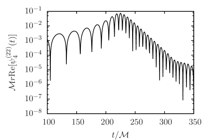
Figure 1: The real part of the $\ell=2$, $m=2$ mode of the Newman-Penrose scalar $\Psi_{4}$, extracted at $r=50\mathcal{M}$. Note the quasinormal ringdown exhibited by the linear decay in the amplitude and the constant frequency on this log-linear plot.

II.4 Scalar evolution in 3+1 form

The scalar field code was developed using Kranc Husa et al. (2006) to generate the initial data and evolution modules and the interface with the BSSN code. A 3+1 decomposition of the scalar wave evolution equation (1) in terms of $\bar{\gamma}_{ij}$, $\bar{K}^{ij}$, $\bar{\alpha}$ and $\bar{\beta}^{i}$ reads:

$$(\partial_{\tau}-\bar{\beta}^{k}\partial_{k})\Phi = \bar{\alpha}\Psi$$ (6)

$$(\partial_{\tau}-\bar{\beta}^{k}\partial_{k})\Psi = \frac{\bar{\alpha}}{\sqrt{\bar{\gamma}}}\partial_{i}(\sqrt{\bar{\gamma}}\bar{\gamma}^{ij}\partial_{j}\Phi)$$ (7)

$$+ \bar{\alpha}\bar{K}\Psi+\bar{\gamma}^{ij}\partial_{i}\bar{\alpha}\partial_{j}\Phi$$

where we have introduced the auxiliary variable $\Psi$ in order to reduce the system to a first-order-in-time form. Notice that we label the time coordinate in the above two equations as $\tau$, in order to stress the distinction between this and the time coordinate $t$ associated with the BBH evolution.

For each of the scalar evolutions, we provide initial data for $\Phi$ and $\Psi$ as follows:

$$\Phi = r^{4}e^{-\frac{(r-r_{0})^{2}}{\sigma^{2}}}\textrm{Re}[Y_{\ell 0}]$$ (8)

$$\Psi = -\frac{2(r-r_{0})}{\alpha\sigma^{2}}\Phi$$ (9)

where $r_{0}=1.6\mathcal{M}$ and $\sigma=1\mathcal{M}$. An outline of our initial setup is provided in figure 2.

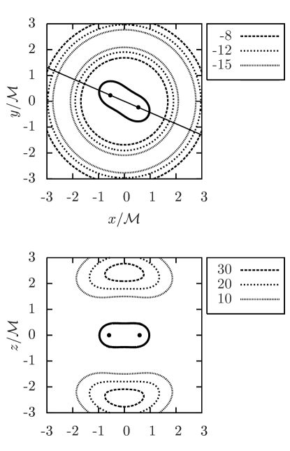
Figure 2: Initial isosurfaces for the scalar field $\Phi$ as in equation (8), in the $\ell=2$ case (broken lines). The solid outline represents the apparent horizon’s intersection with the $xy$-plane (top) and its intersection with the plane containing the $z$-axis and the line connecting the two black hole centers (bottom), at $t=160\mathcal{M}$. Given the initial data for $\Psi$ in equation (9), the two lobes along the z-axis start moving towards the origin. The detector sphere used for extraction is located at $r=5$.

Notice that, as observed in Dorband et al. (2006), the fact that $\textrm{Re}[Y_{\ell m}]=(Y_{\ell m}+Y_{\ell,-m})/2$ implies the concurrent presence of the ($\ell$, $m$) and ($\ell$, $-m$) modes in the initial data. In order to produce ringing waveforms with a single dominant frequency, we chose only $m=0$ modes. Following Dorband et al. Dorband et al. (2006), we extract the multipoles of the scalar field at a coordinate radius $r=5\mathcal{M}$ in all cases (the effect of the extraction radius on the quasinormal frequency is illustrated in section III.3).

II.5 Extracting black hole properties from QNM ringing

In the discussion above, we have mentioned how scalar perturbation theory on a black hole background predicts that, as soon as the initial impulse driving the perturbation propagates away, the scalar field will relax back to its equilibrium configuration through a period of damped (quasinormal) oscillations; numerical simulations (see, e.g., Dorband et al. (2006)) confirm this picture. In the quasinormal regime the scalar field can be quite accurately described in terms of a set of quasinormal modes identified by the three numbers $\ell$, $m$ (labeling the angular eigenstates) and $n$ (labeling the radial eigenstates). In time, each multipole evolves perturbatively, independently of the others and is characterized by a specific complex frequency $\Omega_{\ell mn}$, whose dependence on the black hole mass and spin is known. In principle, then, it should be possible to extract information about the black hole parameters $M$ and $j$ by measuring $\Omega_{\ell mn}$ for a number of different $\ell mn$-modes.

The peculiar nature of quasinormal modes complicates this procedure: since quasinormal modes do not constitute a complete set of eigenstates, they cannot serve as a basis for the solutions of equation (1), and there is no guarantee that, at any given instant of time, the scalar field can be described as a superposition of quasinormal modes alone. However, the practical evidence is that the system will follow a time evolution path which, for some transitory period, will live almost entirely on the subspace spanned by the quasinormal modes Leaver (1986); Berti and Cardoso (2006).

As in Buonanno et al. (2007), we compute the time series $\Phi_{\ell 0}(\tau)$:

$$\Phi_{\ell 0}(\tau) = \int_{S_{\rho}}Y^{*}_{\ell 0}(\theta,\phi)\Phi(\rho,\theta,\phi,\tau)d^{2}\Omega$$ (10)

(where $Y_{\ell 0}$ are the standard (spin zero) spherical harmonics with $m=0$, and the angular modes $\Phi_{\ell 0}$ are extracted on a sphere $S_{\rho}$ of fixed coordinate radius $\rho$), and fit it to a superposition of quasinormal modes:

$$\Phi_{\ell 0}^{\mathrm{{QN}}}(\tau;A,M,j,\phi,\tau_{0})=$$

$$\textrm{Re}\left[\sum_{n}A_{\ell 0n}e^{-i\Omega_{\ell 0n}(M,j)(\tau-\tau_{0})+\phi_{\ell 0n}}\right]$$ (11)

where $A_{\ell 0n}$ and $\phi_{\ell 0n}$ are real constants, and the complex quasinormal frequencies $\Omega_{\ell 0n}(M,j)=\omega_{\ell 0n}(M,j)+i\alpha_{\ell 0n}(M,j)$ depend on $M$ and $j$ in a somewhat complicated way, which can however be represented quite conveniently through the use of tabulated data Berti and Cardoso (2006), complemented with third order interpolation. Note that we only fit to the $m=0$ fundamental mode ($n=0$), however, we study the error associated with not including higher overtones.

In order to extract the black hole parameters we minimize the residual of the fit

$$q(A,M,j,\phi,\tau_{0},\tau_{f})=$$

$$\frac{\int_{\tau_{0}}^{\tau_{f}}d\tau\,|\Phi_{\ell 0}(\tau)-\Phi_{\ell 0}^{\mathrm{QN}}(\tau;A,M,j,\phi,\tau_{0})|}{\int_{\tau_{0}}^{\tau_{f}}d\tau\,|\Phi_{\ell 0}(\tau))|}$$ (12)

with respect to $A$, $M$, $j$ and $\phi$ (with the $M$ and $j$ dependence given by the table interpolation method mentioned above).

As mentioned above, there is no a priori prescription for the initial and final times $\tau_{0}$ and $\tau_{f}$ delimiting the fitting window in which the minimum search is performed. In Dorband et al. (2006) and Buonanno et al. (2007), $\tau_{0}$ is included as an additional fitting parameter, along with some heuristic prescription for $\tau_{f}$. In Berti et al. (2007a), the value of $\tau_{0}$ was obtained by cross-correlating different angular modes, with two different cutoff criteria for $\tau_{f}$. In this work, we start by choosing the initial and final times $\tau_{0}$ and $\tau_{f}$ so that the fitting window excludes the initial prompt response phase and the final wave portion contaminated by numerical and outer boundary error, or $\tau_{0}\sim 25\mathcal{M}$ and $\tau_{f}\sim 55\mathcal{M}$. We then perform a two-dimensional analysis of the variations in the best-fit parameters induced by a change in $\tau_{0}$ and $\tau_{f}$. This analysis provides an estimate of the frequency extraction error and ensures that small variations on either of these parameters have no appreciable influence on the fit results.

As noted in Berti et al. (2007b), the extraction of the complex exponentials from a quasinormal ringing waveform is a delicate procedure. In order to minimize equation (II.5), we have tested the non-linear least-squares Levenberg-Marquardt algorithm, which proved to be inadequate for our purposes. We then chose a fitting algorithm based on an optimization method known as the Covariant Matrix Adaptation Evolutionary Strategy (CMA-ES), whose details can be found in Hansen and Ostermeier (2001) and which is available as a convenient open-source Matlab routine cma . As a consistency check, we have tested the fitting procedure employing CMA-ES, the Matlab Levenberg-Marquardt nlinfit routine, and obtained comparable results whenever the latter routine converged to a minimum. We have also tested CMA-ES on synthetic waveforms such as those discussed in Berti et al. (2007b), obtaining similar results to the Kumaresan-Tufts and matrix pencil methods presented there.

Notice that equation (II.5) involves an infinite set of overtones, i.e. different $n$-modes. In practice, however, the excitation of the vast majority of modes will be highly suppressed, and we will only have to consider the overtones with contributions above the level of numerical error. Recent evidence Buonanno et al. (2007) shows that, even though higher overtones are usually heavily suppressed, their inclusion in the fitting routine noticeably improves the quality of the fit. Since our primary interest is in extraction of the black hole parameters, however, we have decided to focus on the frequency of the fundamental mode alone, choosing a $\tau_{0}$ sufficiently large to effectively guarantee that the contribution of the overtones (which damp quickly) is below our numerical error. We discuss the error contribution from using the fundamental mode below in section III.3.

Other important error sources include the finite radial and angular resolution, the presence of numerical error from finite differencing, and possibly additional effects due to the dynamical slicing of the spacetime which ordinarily occurs during a 3+1 evolution. In order to address these potential issues, in section III.3 we try to quantify their effect. The mass and spin estimates from independent sources also provide evidence that our cumulative error budget is correctly estimated.

III Results

As a first test of the validity of our setup we evolved a single Schwarzschild black hole in isotropic coordinates using the standard moving puncture recipe that leads to coordinate dynamics. We then took snapshots of the gravitational field variables and solved the scalar wave equation numerically on these hypersurfaces and extracted the fundamental quasinormal frequency found in the scattered scalar field for a variety of choices of $\tau_{0}$ and $\tau_{f}$ in Equation (II.5). The values of the real and imaginary part of the quasinormal frequency coincided with the result from perturbation theory up to $\Delta\omega\lesssim 0.002\mathcal{M}^{-1}$ and $\Delta\alpha\lesssim 0.002\mathcal{M}^{-1}$ (which corresponds to $\Delta M\lesssim 0.01\mathcal{M}$ and $\Delta j\lesssim 0.05$ for the $\ell=2$ mode).

In the binary coalescence runs, for all $t\geq 160\mathcal{M}$ a common apparent horizon is present, and becomes approximately axisymmetric at $t\sim 165\mathcal{M}$ (see Dreyer et al. (2003) for a description of the Killing vector field finding algorithm we deployed). Starting at this time, and until after the coalescence is complete (at about $t=260\mathcal{M}$, as indicated by the horizon parameters $M$ and $j$ becoming constant in time), we freeze the gravitational variables at regular intervals and perform an evolution of the scalar field $\Phi$ as described by equation (1) on the corresponding geometry, using the reference resolution of $\mathcal{M}/51.2$.

III.1 Waveforms

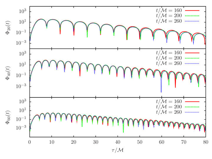
Figure 3: The $\ell=\{2,4,6\}$-modes of the scalar field are shown in the three panels. Each mode was evolved on hypersurfaces extracted at $t=\{160,200,260\}\mathcal{M}$ from a binary black hole inspiral. The modes were obtained on a sphere of constant coordinate radius $\rho=5\mathcal{M}$.

Figure 3 shows the $\ell=\{2,4,6\}$ modes of the scalar field extracted on a coordinate sphere of radius $\rho=5\mathcal{M}$ in separate panels. Each mode was evolved on three different hypersurfaces labeled by $t=\{160,200,260\}\mathcal{M}$ (as stated above, at $t=160\mathcal{M}$ the first common apparent horizon is found, and by $t=260\mathcal{M}$ the system has settled down and we expect to observe the typical evolution of a scalar field scattered from a Kerr black hole). As can be clearly seen from this figure each waveform undergoes a damped oscillatory phase. We observe the emergence of quasinormal ringing on each spatial slice containing a common apparent horizon, regardless of whether the merged system has already settled down ($t=260\mathcal{M}$) or is still evolving very dynamically ($t=160\mathcal{M}$). Initially the scalar field ringing is virtually identical on each of the three hypersurfaces shown, but significant dephasing is obtained towards the end of the scalar field simulation due to the different values of the fundamental frequency in the three cases. This is not an artifact of resolution, but rather shows the difference between the hypersurfaces.

For each time $t$ where we extract a hypersurface snapshot and evolve the scalar field, we fit a quasinormal mode to the scattered scalar field. Figure 4 shows the fit residual $q$ as a function of $t$ for the $\ell=\{2,4,6\}$ modes. This gives us a rough indicator of how well the scattering can be described by quasinormal mode ringing. The fit residual $q$ decreases with increasing $t$, indicating that the evolution on earlier hypersurfaces leads to an inferior fitting quality. This loss in fit quality at early times is reasonable because the scalar field is expected to depart from the familiar quasinormal ringing behavior since earlier hypersurfaces are representing a black hole in more and more dynamical phases. Also note that the higher modes are more difficult to resolve and hence a larger residual is observed.

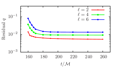
Figure 4: The minimum of the fitting residual $q$ (see Equation (II.5)) as a function of $t$ for the $\ell=\{2,4,6\}$ mode of the scalar field. At early times $t$ the black hole has not yet settled down and hence the fit residual $q$ is larger as the scalar field evolved on the black hole background does not exhibit similarly clean ringdown as it does for later times.

III.2 Black hole parameters extracted from the scalar field probe

Figure 5 shows the black hole mass $M$ and spin $j$ as obtained from the scalar field evolved on different hypersurfaces labeled by $t$, for the $\ell=\{2,4,6\}$ modes. For reference, we also show the values obtained directly from the dynamical horizon finder. Both $M$ and $j$ show qualitatively similar behavior, with an initial transition regime immediately after the first common apparent horizon formation (at $t=160\mathcal{M}$). About $20\mathcal{M}$ after the common apparent horizon is found we can reliably extract the spin and mass of the final black hole from the scattered scalar field.

We want to emphasize that, while the scalar field modes on the different hypersurfaces appear almost identical, the extracted mass and spins show much larger differences due to the strong dependence of $M,j$ on the extracted quasinormal frequency $\Omega_{\ell m}$ (notice that the error bars in figure 5 represent not only the uncertainty associated with the best-fit procedure, but also the contribution to the error due to finite numerical resolution, to angular mode extraction at a finite distance from the black hole and to the choice to neglect any overtones or different angular modes in the frequency extraction; these contributions will be discussed in section III.3).

In the transition regime between $160\mathcal{M}$ and $180\mathcal{M}$ the fit errors (in particular, those from varying the choice of $\tau_{0}$ and $\tau_{f}$) become so large that an accurate extraction of the black hole parameters is not possible anymore. Note that the extraction of $M$ and $j$ at early times is so sensitive to $\tau_{0}$ and $\tau_{f}$ that the associated uncertainty dominates the bars shown in figure 5 for $t\lesssim 180\mathcal{M}$.

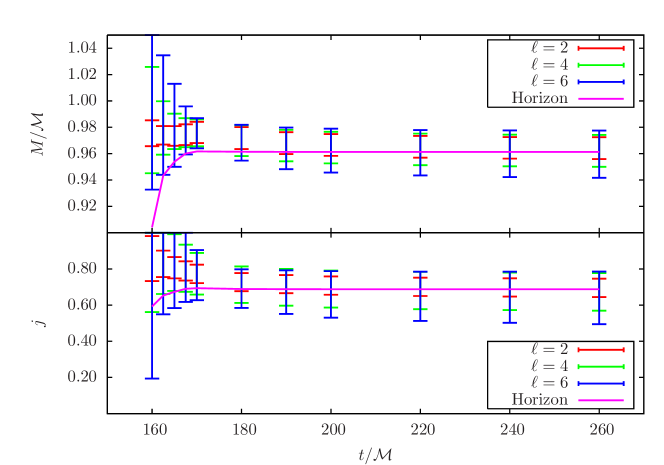
Figure 5: The mass and spin parameters extracted from the fundamental mode frequency, for the three angular modes. The error bars for the horizon mass and spin is included in the curve width. At early times, different choices of $\tau_{0}$ and $\tau_{f}$ lead to significant modifications in the behavior of $M$ and $j$ as a function of $t$. The data error bars in this regime should therefore be considered as an indication of the mass and spin range on each hypersurface.

We conclude that our scattering procedure constitutes an accurate probe of the final black hole potential (defined in the perturbative sense as summarized in section II) at times $t\sim 180\mathcal{M}$, consistent with the results from the isolated horizon parameters. Between $160\mathcal{M}$ and $180\mathcal{M}$, the black hole parameters $M$ and $j$ cannot be reliably extracted; however, the scalar wave is still showing quasinormal ringing. In this regime, due to the level of uncertainty associated with our numerical resolution and frequency extraction routine, we can only provide a broad constraint for the extracted parameters.

III.3 Effect of finite resolution, extraction radius and number of fitting modes

At this point we would like to discuss the different error sources for the final extraction of the black hole parameters $M$ and $j$ from the scalar field waveforms. We discuss how sensitive the extraction of these parameters is to the fit range $[\tau_{0},\tau_{f}]$, to resolution, to wave extraction radius and to fitting the waveform to a superposition of more than one quasinormal mode. It is important to keep in mind that the black hole mass and spin parameters show a strong dependence on the scalar quasinormal frequencies $\Omega$ and hence a small fractional error in $\Omega$ translates into a much amplified fractional error in $M$ and, especially, $j$.

In order to provide a description of the fitting error, especially due to the choice of the fitting window $[\tau_{0},\tau_{f}]$, we select $\tau_{0}=25\mathcal{M}$ and $\tau_{f}=55\mathcal{M}$ as reference values and vary these two parameters over a $10\mathcal{M}$-wide interval centered around each. The induced variation in $M$ and $j$ is illustrated in figure 6 for a few representative cases: this estimate provides a quantitative range for the uncertainty in the fitting parameters. In the following, we limit ourselves to this pair of reference values and quote the error associated with this choice.

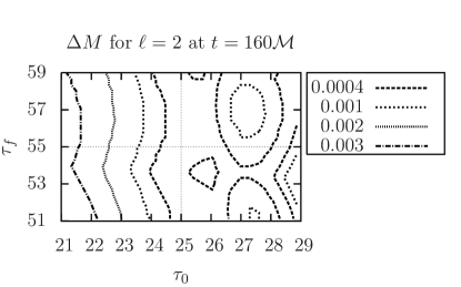
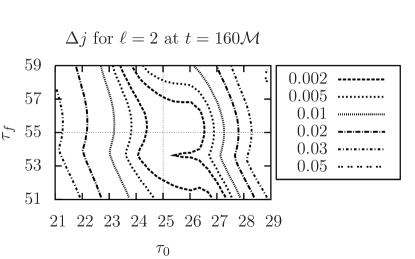
Figure 6: Contours of the variation of the mass estimate $\Delta M(\tau_{0},\tau_{f})=|M(\tau_{0},\tau_{f})-M(25\mathcal{M},55\mathcal{M})|$ and spin estimate $\Delta j(\tau_{0},\tau_{f})=|j(\tau_{0},\tau_{f})-j(25\mathcal{M},55\mathcal{M})|$ for $\ell=2$ at $t=160\mathcal{M}$, as a function of $\tau_{0}$ and $\tau_{f}$. The other cases follow similar patterns, with error ranges improving at later times and degrading for higher $\ell$-modes.

For the three different resolutions listed above ($h=\mathcal{M}/44.8$, $\mathcal{M}/51.2$ and $\mathcal{M}/57.6$), we find that both the real and the imaginary part of the extracted frequencies exhibit a monotonic trend as $h$ decreases, with the difference between neighboring resolutions decreasing as $h\to 0$ and the difference between the highest and the lowest resolution remaining always under $0.0003\mathcal{M}^{-1}$. As for the extraction radius, the six different choices ($\rho=10\mathcal{M},20\mathcal{M},\dots,50\mathcal{M}$ in addition to the initial $\rho=5\mathcal{M}$) lead to frequency shifts of the order of $0.005\mathcal{M}^{-1}$. The uncertainty is also smaller if the extraction is performed on detectors that are farther from outer and refinement boundaries, such as the ones at $5\mathcal{M}$, $10\mathcal{M}$ and $30\mathcal{M}$ (the different spatial resolutions characteristic of different extraction radii are not dramatically relevant, indicating that the modes are well resolved in all the cases considered).

Finally, the actual eigenfunctions of the angular part of the wave operator in equation (1) on a Kerr spacetime are the (spin-zero) spheroidal harmonics $S_{\ell m}$, rather than the spherical harmonics $Y_{\ell m}$ used here; however, as discussed in Press and Teukolsky (1973), $Y_{\ell m}=S_{\ell m}+(a^{2}|\Omega|^{2})\sum_{\ell^{\prime}\neq l}B_{\ell^{\prime}m}S_{\ell^{\prime}m}+O(a^{4}|\Omega|^{4})$, so that the use of spherical harmonics only causes a modest amount of mode mixing in the extracted waveforms (additionally, Berti et al. Berti et al. (2006b) find that this expansion is surprisingly accurate out to values of $a|\Omega|$ close to unity). To determine the bias caused by such mode mixing on the best-fit value of the fundamental frequency, we extend the fitting function (II.5) to a superposition of two and three different angular modes. The change in the complex frequency of the fundamental mode due to the inclusion of a different number of modes is under $0.0006\mathcal{M}^{-1}$. Unlike the error due to the frequency fitting, these last three sources of error have virtually no fluctuations from hypersurface to hypersurface. For all times, the cumulative errors associated with the determination of the complex frequency (including the last three sources of error but not the uncertainty introduced by the fitting procedure) then amount to $\sim 0.005\mathcal{M}^{-1}$. This number is propagated to $M$ and $j$ via $\Delta M=M(\Omega+\Delta\Omega)-M(\Omega)$ and $\Delta j=j(\Omega+\Delta\Omega)-j(\Omega)$ which yields:

$\Delta M=0.02\mathcal{M}$	,	$\Delta j=0.1$		for $\ell=2$
$\Delta M=0.02\mathcal{M}$	,	$\Delta j=0.15$		for $\ell=4$
$\Delta M=0.03\mathcal{M}$	,	$\Delta j=0.2$		for $\ell=6$  .

Finally, these numbers are summed in quadrature to the errors in $M$ and $j$ due to the fitting procedure (shown in figure 6), yielding the error bars in figure 5.

IV Discussion and conclusions

In the previous section, we have presented the result of an experiment involving the scattering of a massless scalar field off the curvature of a spacetime containing two coalescing black holes. This spacetime was generated numerically by a full 3D black hole simulation following the moving puncture paradigm. Each spatial hypersurface obtained served as a fixed background for the propagation of the scalar field as described in section II.2 and the behavior of the scalar field was analyzed in each case.

We observed the emergence of quasinormal ringing on each spatial slice containing a common apparent horizon regardless of whether the merged system had already settled down to a single Kerr black hole. While we could not reliably extract the final black hole parameters immediately after the formation of a common apparent horizon ($t=160\mathcal{M}$), we could still clearly identify quasinormal ringing even in this early phase where the merged black hole is strongly excited and the scattering potential deviates from that of Kerr. This finding agrees with earlier results where scalar perturbations on Vaidya spacetimes were studied and quasinormal ringing could be identified even on time-dependent black hole backgrounds Shao et al. (2005). Our results and interpretation are also consistent with the evidence from the Close Limit approximation Price and Pullin (1994), where a pair of black holes in a head-on collision was shown to have already entered the perturbative regime when a common apparent horizon surrounded them. Based on this observation, the scattering of a test scalar field from the merged black hole could provide information about the final black hole state before the spacetime has settled down to its final state.

Soon after horizon formation (i.e. for times $t\gtrsim 180\mathcal{M}$) we were able to obtain estimates for the mass and spin of the final black hole from the scalar field probe in good agreement with direct isolated horizon measures. This indicates that, at this time, the dynamics surrounding the black hole has settled down sufficiently that the scattering potential for the scalar field is essentially that of the final black hole, even though there is still non-trivial dynamics in the vicinity of the horizon.

A more exhaustive analysis of the early-time scalar quasinormal ringing waveforms before $t=180\mathcal{M}$ is necessary to obtain more conclusive results in the non-linear, merger phase, and is left for future work.