Photoconductivity of an intrinsic graphene

Abstract

We examine the photoconductivity of an intrinsic graphene associated with far- and mid-infrared irradiation at low temperatures. The model under consideration accounts for the excitation of the electron-hole pairs by incident radiation, the interband generation-recombination transitions due to thermal radiation, and the intraband energy relaxation due to acoustic phonon scattering. The momentum relaxation is assumed to be caused by elastic scattering. The pertinent collision integrals are adapted for the case of the massless energy spectrum of carriers that interact with the longitudinal acoustic mode and the thermal radiation. It is found that the photoconductivity is determined by interplay between weak energy relaxation and generation-recombination processes. Due to this the threshold of nonlinear response is fairly low.

I Introduction

There are two reasons for unusual transport properties of graphene (see Refs.  1 ; 2 ): the neutrinolike dynamics of carriers, which is described by the Weyl-Wallace model, 3 and the specific features of scattering processes. In particular, the high efficiency of interband optical transitions is associated with a high value of the velocity $v_{\scriptscriptstyle W}\simeq 10^{8}$ cm/s characterizing the linear dispersion relations for the graphene valence and conduction bands. This is because the matrix element of interband transitions is proportional to $v_{\scriptscriptstyle W}$. On the other hand, the coupling of carriers to acoustic phonons appears to be weak. As a result, non-equilibrium distributions of photoexcited carriers can readily be realized for the energies smaller than the optical phonon energy in the low-temperature region. Due to this, a photoresponse of graphene to far- and mid-infrared (IR) irradiations should be strong and a low threshold of nonlinear response takes place. To the best of our knowledge, the effects of non-equilibrium carriers under far- or mid-IR excitations is not considered before: both experimental and theoretical studies of the transport phenomena in graphene are performed at weak dc electric fields (see 4 and 5 ; 6VR respectively) or under optical excitation (see 6opt and references therein).

In this paper, we study the far- and mid-IR photoconductivities of an intrinsic graphene at low temperatures. As known, 4 ; 5 ; 6VR the intrinsic graphene exhibits a maximum of the dark resistance. Hence, the effect of photoconductivity of such a material should be fairly strong. Since the concentration of carriers in the intrinsic graphene at low temperatures is rather small (less $10^{10}$ cm^-2 at 100 K and lower), one can disregard the intra- and interband Coulomb scattering processes. Thus, considering the photoresponse of the intrinsic graphene at low-temperatures one needs to take into account the following mechanisms [see Fig. 1(a)]:
(1) the far- or mid-IR interband photoexcitation;
(2) the generation-recombination processes due to the interband transitions caused by thermal radiation;
(3) the intraband quasi-elastic scattering on acoustic phonons;
(4) the scattering due to a static disorder which is an essential mechanism of the momentum relaxation. 2 ; 4 ; 5 ; 6VR

Figure 1: (a) Schematic view of the interband and intraband transitions under consideration. (b) The distribution functions of thermalized and photoexcited carriers, $f_{p}^{\scriptscriptstyle(eq)}$ and $\Delta f_{p}$ (dashed and solid curves, respectively), in the intrinsic graphene at low temperatures. Dotted peaks show photoexcited carriers distribution.

The shape of the non-equilibrium energy distribution of carriers is determined by interplay between the radiative generation-recombination processes and the quasi-elastic energy relaxation. Indeed, the corresponding relaxation rates, as we will show below, are of the same order at the temperatures about 100 K and lower. Since both rates are proportional to the density of states and the radiative transitions are temperature-independent, the generation-recombination processes not only determine the carrier concentration but also affect the carrier energy distribution. Due to an effective recombination of low-energy carriers, their energy distribution might become nonmonotonic exhibiting a peak as shown in Fig. 1(b). Here we restrict ourselves to the linear (with respect to pumping intensity) response. The photoconductivity appears to be proportional to the concentration of the photogenerated carriers for the case of short-range momentum relaxation. This concentration as well as the photoconductivity decrease with the temperature and the energy of the photoexcitation. However, these dependencies are different if the long-range momentum relaxation is essential.

The paper is organized as follows. The basic equations governing the photoconductivity in graphene are presented in Sec. II. In Sec. III, we consider the carrier distribution for the case of linear (with respect to the photoexcitation rate) response. The results of calculations of the photoconductivity in this case, including numerical estimates, are presented in Sec. IV. The concluding remarks and discussion of the assumptions used are given in Sec. V. In Appendix, the collision integrals for the interband relaxation associated with thermal radiation and for the intraband relaxation caused by acoustic phonons are derived.

II Basic equations

We describe the linear response of photoexcited carriers to the dc electric field ${\bf E}_{0}$ using the steady state kinetic equation for the distribution function $F_{l{\bf p}}$: 7mono

$$e{\bf E_{0}}\cdot\frac{\partial F_{l{\bf p}}}{\partial{\bf p}}=\sum_{j}J_{j}\{F|l{\bf p}\}+G\{F|l{\bf p}\}.$$ (1)

Here $l$ corresponds to conduction ($l$=+1) or valence ($l$=-1) band, ${\bf p}$ is the 2D momentum, $J_{j}\{F|l{\bf p}\}$ is the collision integral for the $j$th scattering mechanism, ($j=D,~{}LA$, and $R$ correspond to the static disorder, the acoustic phonon scattering, or the radiative-induced interband transitions, respectively), and $G\{F|l{\bf p}\}$ is the interband photogeneration rate. Below we restrict ourselves by the weak dc field case, so that $F_{l{\bf p}}\simeq F_{lp}+\Delta F_{l{\bf p}}$, where $F_{lp}$ is the symmetric part of the distribution function under the photoexcitation and $\Delta F_{l{\bf p}}\propto E_{0}$ is the asymmetric addition. We evaluate the in-plane isotropic generation rate, present the kinetic equation that governs the distributions functions $F_{lp}$, and discuss the expression for the conductivity considered in 6VR .

II.1 Interband photoexcitation rate

Within the framework of the Weyl-Wallace model, the carrier dynamics under the in-plane ac electric field ${\bf E}_{\omega}\exp(-i\omega t)+c.c.$ with the frequency $\omega$ is described by the zero-field Hamiltonian $\hat{h}_{\scriptscriptstyle W}=v_{\scriptscriptstyle W}(\hat{\mbox{\boldmath$\sigma$}}\cdot{\bf p})$ with the pseudospin Pauli matrix $\hat{\mbox{\boldmath$\sigma$}}$ and the harmonic perturbation operator:

$$\frac{iev_{\scriptscriptstyle W}}{\omega}(\hat{\mbox{\boldmath$\sigma$}}\cdot{\bf E}_{\omega})e^{-i\omega t}+c.c.~{}.$$ (2)

Following the general consideration of interband photoexcitation (see Sec. 53 in Ref. 8), one can obtain the interband photogeneration rate into the $l{\bf p}$-state in the form:

$$G\{F|l{\bf p}\}=\frac{2\pi}{\hbar}\biggl{(}\frac{ev_{\scriptscriptstyle W}}{\omega}\biggr{)}^{2}\sum_{l^{\prime}{\bf p}^{\prime}}|(l{\bf p}|\hat{\mbox{\boldmath$\sigma$}}{\bf\cdot E}_{\omega}|l^{\prime}{\bf p}^{\prime})|^{2}(F_{l^{\prime}{\bf p}^{\prime}}-F_{l{\bf p}})$$

$$\times[\delta_{\gamma}\left(\varepsilon_{l{\bf p}}-\varepsilon_{l^{\prime}{\bf p}^{\prime}}-\hbar\omega\right)+\delta_{\gamma}(\varepsilon_{l{\bf p}}-\varepsilon_{l^{\prime}{\bf p}^{\prime}}+\hbar\omega)],~{}~{}~{}~{}$$ (3)

where the energy conservation law has been introduced via the function $\delta_{\gamma}(\varepsilon)$ with the phenomenological broadening energy $\gamma$. 8broad

Next, we neglect the in-plane anisotropy of $F_{l{\bf p}}$ assuming that the dc electric field ${\bf E_{0}}$ is sufficiently weak, so that one can perform the averaging of the matrix element in Eq. (3) over the in-plane angle: 9eg $\overline{\left|\langle\pm 1,{\bf p}|\hat{\sigma}_{x,y}|\mp 1,{\bf p}\rangle\right|^{2}}=1/2$. As a result, the generation rate in $l$th band takes form:

$$G\{F|l{\bf p}\}=\frac{\pi}{\hbar}\left(\frac{ev_{\scriptscriptstyle W}E_{\omega}}{\omega}\right)^{2}\left(F_{-lp}-F_{lp}\right)$$

$$\times\delta_{\gamma}\left(\varepsilon_{lp}-\varepsilon_{-lp}-l\hbar\omega\right)$$ (4)

with $G\{F_{+l{\bf p}}\}+G\{F_{-l{\bf p}}\}=0$ due to the conservation of the net number of the carriers. It is convenient to use in the following the electron-hole representation that introduces the electron ($e$) and hole ($h$) distribution functions according to the standard replacements 10 :

$$F_{+1,{\bf p}}\rightarrow f_{e{\bf p}},\qquad 1-F_{-1,{\bf p}t}\rightarrow f_{h{\bf p}}.$$ (5)

Considering this substitution, we obtain $G\{F|+l{\bf p}\}\rightarrow G\{f|p\}$ and $G\{F|-1,p\}\rightarrow-G\{f|p\}$ with the same generation rate:

$$G\{f|p\}=\frac{\pi}{\hbar}\left(\frac{ev_{\scriptscriptstyle W}E_{\omega}}{\omega}\right)^{2}\left(1-f_{ep}-f_{hp}\right)\delta_{\gamma}\left(2v_{\scriptscriptstyle W}p-\hbar\omega\right),$$ (6)

which is symmetric with respect to the electron-hole replacement, $f_{ep}\leftrightarrow f_{hp}$.

Considering the case of relatively weak excitation, we assume in the following that $f_{e,hp}\ll 1$ in the vicinity of $p_{\omega}\equiv\hbar\omega/2v_{\scriptscriptstyle W}$. For such a case, $G(f|p)\simeq G_{p}$ and $G_{p}$ are independent of the carrier distribution:

$$G_{p}=\nu_{\scriptscriptstyle E}\Delta\left(\frac{p-p_{\omega}}{\delta p}\right),~{}~{}~{}~{}\nu_{\scriptscriptstyle E}=\frac{\pi}{\hbar\gamma}\left(\frac{ev_{\scriptscriptstyle W}E}{\omega}\right)^{2}.$$ (7)

Here $\Delta(E)\equiv\gamma\delta_{\gamma}(E)$, $\delta p\equiv\gamma/2v_{\scriptscriptstyle W}$ and $\nu_{\scriptscriptstyle E}$ is the photoexcitation frequency. By disregarding the intraband photoexcitation of electrons and holes, i.e. the Drude mechanism of photoexcitation, we suppose that $\delta p\ll p_{\omega}$ or $\gamma\ll\hbar\omega$.

II.2 Kinetic equation for $f_{p}$

Since the collision integrals [see Eqs. (A.8) and (A.12) in Appendix A] preserve their form when $f_{ep}$ is replaced by $f_{hp}$, the electron and hole distributions in the intrinsic material under the photoexcitation are identical (see Fig. 1). In addition, the elastic scattering does not affect the symmetric distribution due to the energy conservation. As a result, the kinetic equation for $f_{ep}=f_{hp}\equiv f_{p}$ takes form:

$$J_{\scriptscriptstyle LA}\{f|p\}+J_{\scriptscriptstyle R}\{f|p\}+G_{p}=0.$$ (8)

Here the terms $J_{\scriptscriptstyle LA}$ and $J_{\scriptscriptstyle R}$ describe the relaxation of electrons (holes) caused by the phonon and photon thermostats with the lattice temperature $T$. These terms are calculated in Appendix. The term associated with the interband contribution $J_{\scriptscriptstyle R}\{f|p\}$ can be presented as

$$J_{\scriptscriptstyle R}\{f|p\}=\nu_{p}^{\scriptscriptstyle(-)}(1-f_{p})^{2}-\nu_{p}^{\scriptscriptstyle(+)}f_{p}^{2},$$ (9)

$$\nu_{p}^{(\pm)}=\nu_{p}^{\scriptscriptstyle(R)}\left(N_{2p/p_{\scriptscriptstyle T}}+1/2\pm 1/2\right),$$

where the generation (or recombination) rate, $\nu_{p}^{\scriptscriptstyle(+)}$ (or $\nu_{p}^{\scriptscriptstyle(-)}$), is expressed via the Planck function $N_{2p/p_{\scriptscriptstyle T}}=[\exp(2p/p_{\scriptscriptstyle T})-1]^{-1}$, where $p_{\scriptscriptstyle T}=T/v_{\scriptscriptstyle W}$ is the characteristic thermal momentum. The rate of spontaneous radiative transitions, $\nu_{p}^{\scriptscriptstyle(R)}$, is presented [see Eqs. (A.5) and (A.6) in Appendix] as follows:

$$\nu_{p}^{\scriptscriptstyle(R)}=\frac{e^{2}\sqrt{\epsilon}}{\hbar c}\left(\frac{v_{\scriptscriptstyle W}}{c}\right)^{2}\frac{8v_{\scriptscriptstyle W}p}{3\hbar}\equiv\frac{v_{r}p}{\hbar}$$ (10)

where $\epsilon$ is the dielectric permittivity. Here, we have introduced the characteristic radiative velocity $v_{r}$.

To derive the expression for the in-plane isotropic collision integral $J_{\scriptscriptstyle LA}\{f|p\}$ from (A.12), it is convenient to transform the transition probabilities (A.11) into $\overline{W}_{{\bf pp}^{\prime}}=(W_{{\bf pp}^{\prime}}+W_{{\bf p}^{\prime}{\bf p}})/2$ and $\Delta W_{{\bf pp}^{\prime}}=W_{{\bf pp^{\prime}}}-W_{{\bf p^{\prime}p}}$, so that $J_{\scriptscriptstyle LA}\{f|{\bf p}\}$ can be presented as:

$$J_{\scriptscriptstyle LA}\{f|{\bf p}\}=\sum_{{\bf p^{\prime}}}\overline{W}_{\bf pp^{\prime}}\left(f_{\bf p^{\prime}}-f_{\bf p}\right)~{}~{}~{}~{}~{}$$ (11)

$$-\frac{1}{2}\sum_{{\bf p^{\prime}}}\Delta W_{\bf pp^{\prime}}\left[(1-f_{\bf p})f_{\bf p^{\prime}}+(1-f_{\bf p^{\prime}})f_{\bf p}\right].$$

The energy transfer described by Eq. (A.11) is small because $s\ll v_{\scriptscriptstyle W}$ where $s$ is the sound velocity. By using also the in-plane averaging $\overline{\Psi(\widehat{{\bf p},{\bf p}^{\prime}})|{\bf p}-{\bf p}^{\prime}|^{2}}=(p^{2}+p^{\prime 2}-pp^{\prime})/2$, where the overlap factor $\Psi\left(\widehat{{\bf p^{\prime}},{\bf p}}\right)$ is given by Eq. (A.10), one obtains the transition probabilities:

$$\left|{\begin{array}[]{*{20}c}{\overline{W}_{{\bf pp}^{\prime}}}\\ {\Delta W_{{\bf pp}^{\prime}}}\\ \end{array}}\right|\simeq\frac{{\pi D^{2}}}{{\hbar\rho_{s}L^{2}}}\frac{{p^{2}+p^{\prime 2}-pp^{\prime}}}{2v_{\scriptscriptstyle W}^{2}}\left|{\begin{array}[]{*{20}c}{p_{\scriptscriptstyle T}\frac{d^{2}}{dp^{\prime 2}}\delta(p-p^{\prime})}\\ \\ {2\frac{d}{{dp^{\prime}}}\delta(p-p^{\prime})}\\ \end{array}}\right|,$$ (12)

where $D$ is the deformation potential, $\rho_{s}$ is the sheet density of graphene and $L^{2}$ is the normalization area. Substituting Eq. (12) into Eq. (11) and integrating by parts give us the collision integral in the Fokker-Planck form 7mono ; 11pk :

$$J_{\scriptscriptstyle LA}\{f|p\}=\frac{\nu_{p}^{\scriptscriptstyle(qe)}}{p^{2}}\frac{d}{dp}\left\{p^{4}\left[\frac{df_{p}}{dp}+\frac{f_{p}(1-f_{p})}{p_{\scriptscriptstyle T}}\right]\right\},$$

$$\nu_{p}^{\scriptscriptstyle(qe)}=\left(\frac{s}{v_{\scriptscriptstyle W}}\right)^{2}\frac{v_{ac}p}{\hbar},~{}~{}~{}v_{ac}=\frac{D^{2}T}{4\hbar^{2}\rho_{s}v_{\scriptscriptstyle W}s^{2}}.~{}~{}~{}$$ (13)

Here, we have introduced the rate of energy relaxation, $\nu_{p}^{\scriptscriptstyle(qe)}$, and the characteristic velocity $v_{ac}$ [compare to Eq. (10)].

Since the collision integral (13) is proportional to $p^{-1}d\{\ldots\}/dp$, the integration of the kinetic equation (8) over the $p$-axis yields the following normalization condition:

$$\int_{0}^{\infty}dp\rho_{p}J_{\scriptscriptstyle R}\{f|p\}+\rho_{p_{\omega}}\nu_{\scriptscriptstyle E}\delta p=0,$$ (14)

where $\rho_{p}=2p/\pi\hbar^{2}v_{\scriptscriptstyle W}$ is the density of states in graphene. Deriving Eq. (14), we have used $\int_{0}^{\infty}dp\rho_{p}\Delta[(p-p_{\omega})/\delta p]\simeq\rho_{p_{\omega}}\delta p$ if $\delta p\ll p_{\omega}$.

II.3 Conductivity

The asymmetric parts of electron and hole distribution functions have similar form, and $\Delta f_{e\mathbf{p}}=\Delta f_{h\mathbf{p}}\equiv\Delta f_{\mathbf{p}}$ is given by

$$\Delta f_{\mathbf{p}}=-\frac{(e\mathbf{E}\cdot\mathbf{p})}{p}\tau_{p}^{\scriptscriptstyle(m)}\left(-\frac{df_{p}}{dp}\right).$$ (15)

Here $\left[\tau_{p}^{\scriptscriptstyle(m)}\right]^{-1}=v_{d}p\Psi(pl_{c}/\hbar)/\hbar$ is the momentum relaxation time, where $v_{d}$ and $\Psi(pl_{c}/\hbar)$ characterize the strength of disorder and the quenching of the long-range scattering. If a random potential, $U_{\bf x}$, is characterized by the correlation function $\langle U_{\bf x}U_{\bf x^{\prime}}\rangle\equiv\overline{U_{d}}^{2}\exp\{-[({\bf x}-{\bf x^{\prime}})/l_{c}]^{2}\}$ with the averaged energy $\overline{U_{d}}$ and the correlation length $l_{c}$, 6VR one obtains

$$v_{d}=\frac{\pi\overline{U}_{d}^{2}l_{c}^{2}}{4\hbar^{2}v_{\scriptscriptstyle W}},~{}~{}~{}~{}\Psi(z)=\frac{e^{-z^{2}}}{z^{2}}I_{1}\left(z^{2}\right),$$ (16)

where $I_{1}(x)$ is the first-order Bessel function of an imaginary argument.

The conductivity, $\sigma$, is determined by the standard formula 10

$$\sigma=\frac{4e^{2}v_{\scriptscriptstyle W}}{L^{2}}\sum_{\mathbf{p}}\tau_{p}^{(m)}\left(-\frac{df_{p}}{dp}\right),$$ (17)

where the nonequilibrium distribution $f_{p}$ is determined by Eq. (8). Using the relaxation time $\tau_{p}^{(m)}$ introduced by Eqs. (15) and (16) and integrating by parts in Eq. (17), the conductivity can be presented as follows:

$$\sigma=\frac{e^{2}}{\pi\hbar}\frac{2v_{\scriptscriptstyle W}}{v_{d}}\left[2f_{p=0}+\frac{l_{c}}{\hbar}\int\limits_{0}^{\infty}dpf_{p}\Phi\left(\frac{pl_{c}}{\hbar}\right)\right].$$ (18)

Here, we have introduced the function $\Phi(z)=-\Psi^{\prime}(z)/\Psi(z)^{2}$ and take into account $\Psi(0)=1/2$. In the case of short-range scattering, $p_{\scriptscriptstyle T}l_{c}/\hbar\ll 1$, for the equilibrium conductivity, which corresponds to the distribution $f_{p}^{\scriptscriptstyle(eq)}=[\exp(p/p_{\scriptscriptstyle T})+1]^{-1}$, one obtains $\sigma_{eq}\simeq(e^{2}/\pi\hbar)2v_{\scriptscriptstyle W}/v_{d}$.

III Nonequilibrium distribution

Collecting Eqs. (7-9) and (13) together, we arrive at the equation for the symmetric distribution function $f_{p}$:

$$\frac{\nu_{p}^{\scriptscriptstyle(qe)}}{p^{2}}\frac{d}{{dp}}p^{4}\left[\frac{df_{p}}{dp}+\frac{f_{p}(1-f_{p})}{p_{\scriptscriptstyle T}}\right]+\nu_{p}^{\scriptscriptstyle(\scriptscriptstyle R)}\left[N_{2p/p_{T}}(1-f_{p})^{2}\right.$$

$$\left.-(N_{2p/p_{T}}+1)f_{p}^{2}\right]+\nu_{\scriptscriptstyle E}\Delta\left({\frac{p-p_{\omega}}{{\delta p}}}\right)=0,~{}~{}~{}~{}~{}$$ (19)

which should be solved with the zero-flow boundary condition, $[df_{p}/dp+f_{p}(1-f_{p})/p_{\scriptscriptstyle T}]_{p\rightarrow\infty}=0$, and the normalization condition (14). Since the interband photogeneration is centered in the narrow region $|p-p_{\omega}|\leq\delta p$, one can integrate Eq. (19) over this region. Neglecting an exponentially weak flow at $p>p_{\omega}$, we consider below the uniform equation (19), without the generation term proportional to $\nu_{\scriptscriptstyle E}$. Instead of the generation contribution, we use the boundary condition:

$$\left[\frac{df_{p}}{dp}+\frac{f_{p}(1-f_{p})}{p_{\scriptscriptstyle T}}\right]_{p=p_{\omega}}=\frac{\nu_{\scriptscriptstyle E}\delta p}{\nu_{p_{\omega}}^{\scriptscriptstyle(qe)}p_{\omega}^{2}}$$ (20)

At low pumping, when $f_{p}\simeq f_{p}^{(eq)}+\Delta f_{p}$ and $\Delta f_{p}\ll 1$ ($\Delta f_{p}\propto\nu_{\scriptscriptstyle E}$), Eqs. (19) and (20) can be presented as

$$\frac{d}{{dp}}p^{4}\left[{\frac{{d\Delta f_{p}}}{{dp}}+\frac{{\Delta f_{p}}}{{p_{\scriptscriptstyle T}}}\tanh\left({\frac{p}{{2p_{\scriptscriptstyle T}}}}\right)}\right]$$

$$-\frac{{v_{r}p^{2}}}{{v_{qe}\sinh(p/p_{T})}}\Delta f_{p}=0,$$ (21)

$$\left(\frac{d\Delta f_{p}}{{dp}}+\frac{\Delta f_{p}}{p_{\scriptscriptstyle T}}\right)_{p=p_{\omega}}=\frac{{\nu_{\scriptscriptstyle E}\delta p}}{{\nu_{p_{\omega}}^{(qe)}p_{\omega}^{2}}}.$$

Simultaneously, the normalization condition (14) takes form:

$$\int_{0}^{p_{\omega}}dp\frac{dpp\nu_{p}^{\scriptscriptstyle(R)}}{\cosh(p/p_{\scriptscriptstyle T})}\Delta f_{p}=\nu_{\scriptscriptstyle E}\delta pp_{\omega}.$$ (22)

In the region $p\gg p_{\scriptscriptstyle T}$, where $\tanh(p/2p_{\scriptscriptstyle T})\approx 1$ and $\sinh(p/p_{\scriptscriptstyle T})\approx e^{p/p_{\scriptscriptstyle T}}/2$, one can neglect $(d\Delta f_{p}/dp)$ in comparison to $\Delta f_{p}/p_{\scriptscriptstyle T}$. Consequently, a slow tail of the energy distribution can be governed by the first order equation obtained from Eq. (21). The boundary condition assumes the form $\Delta f_{p=p_{\omega}}=\Delta f_{\omega}$ with

$$\Delta f_{\omega}\simeq\frac{\nu_{\scriptscriptstyle E}\delta pp_{\scriptscriptstyle T}}{\nu_{p_{\omega}}^{\scriptscriptstyle(qe)}p_{\omega}^{2}}.$$ (23)

By introducing a connection point $p_{c}$ according to $p_{\scriptscriptstyle T}\ll p_{c}\ll p_{\omega}$, we obtain the following slow-varying solution for the interval $p_{c}<p<p_{\omega}$:

$$\frac{\Delta f_{p}}{\Delta f_{\omega}}\simeq\left(\frac{p_{\omega}}{p}\right)^{4}\exp\left(-\frac{{2p_{\scriptscriptstyle T}v_{r}}}{{v_{qe}}}\int\limits_{p}^{p_{\omega}}\frac{dp_{1}}{p_{1}^{2}}e^{-p_{1}/p_{\scriptscriptstyle T}}\right)~{}~{}~{}$$ (24)

$$=\left({\frac{{p_{\omega}}}{p}}\right)^{4}\exp\left[{-\frac{{2v_{r}}}{{v_{qe}}}\left({\frac{{p_{\scriptscriptstyle T}}}{p}}\right)^{2}\left({e^{-p/p_{\scriptscriptstyle T}}-e^{-p_{\omega}/p_{\scriptscriptstyle T}}}\right)}\right].$$

For the low-energy region, $p<p_{c}$, we search a solution in the form

$$\Delta f_{p}=\exp\left[{-\frac{1}{2}\int{dp\left({\frac{4}{p}+\frac{\tanh(p/2p_{T})}{p_{\scriptscriptstyle T}}}\right)}}\right]\delta f_{p}$$

$$\approx\frac{{(p_{\scriptscriptstyle T}/p)^{2}}}{\cosh(p/2p_{\scriptscriptstyle T})}\delta f_{p},~{}~{}~{}~{}~{}~{}$$ (25)

where $\delta f_{p}$ is governed by the second order equation

$$\frac{{d^{2}\delta f_{p}}}{{dp^{2}}}-\frac{{v_{r}/v_{qe}}}{p^{2}\sinh(p/p_{\scriptscriptstyle T})}\delta f_{p}=0$$ (26)

with the parameter $v_{r}/v_{qe}\gg 1$. Within the WKB approximation 12wkb , we obtain the solution of Eq. (26) in the form:

$$\delta f_{p}\simeq C\exp\left[-\sqrt{\frac{v_{r}}{v_{qe}}}\int\limits_{p}^{p_{c}}{\frac{dp_{1}}{p_{1}\sqrt{\sinh(p_{1}/p_{\scriptscriptstyle T})}}}\right],$$ (27)

where the normalization constant $C$ is determined from the continuity condition at $p=p_{c}$ which is transformed into $(p_{\scriptscriptstyle T}/p_{c})^{2}\delta f_{p_{c}}=\Delta f_{p_{c}}\cosh(p_{c}/2p_{\scriptscriptstyle T})$.

As a result, the photoexcited distribution takes the form:

$$\frac{\Delta f_{p}}{\Delta f_{\omega}}\approx\left\{\begin{array}[]{l}\left(\frac{p_{\omega}}{p}\right)^{4}\exp\left[-\frac{2v_{r}}{v_{qe}}\left(\frac{p_{\scriptscriptstyle T}}{p}\right)^{2}\left(e^{-p/p_{\scriptscriptstyle T}}-e^{-p_{\omega}/p_{\scriptscriptstyle T}}\right)\right],\\ ~{}~{}~{}~{}~{}~{}~{}~{}~{}~{}p_{c}<p<p_{\omega},\\ ~{}~{}~{}~{}~{}\{A_{c}p_{\omega}^{4}/[2p_{c}^{2}p^{2}\cosh(p/2p_{\scriptscriptstyle T})]\}\\ \times\exp\left[-\sqrt{\frac{v_{r}}{v_{qe}}}\int\limits_{p}^{p_{c}}{\frac{dp_{1}}{p_{1}\sqrt{\sinh(p_{1}/p_{\scriptscriptstyle T})}}}\right],\\ ~{}~{}~{}~{}~{}~{}~{}~{}~{}~{}0<p<p_{c},\end{array}\right.$$ (33)

where

$$A_{c}\simeq\exp\left[\frac{p_{c}}{2p_{\scriptscriptstyle T}}-\frac{2v_{r}}{v_{qe}}\left(\frac{p_{\scriptscriptstyle T}}{p_{c}}\right)^{2}e^{-p_{c}/p_{\scriptscriptstyle T}}\right].$$ (34)

The connection point $p_{c}$ in the distribution (28) is determined by

$$\frac{v_{qe}}{v_{r}}=\frac{A_{c}}{2}\left(\frac{p_{\scriptscriptstyle T}}{p_{c}}\right)^{2}\int\limits_{0}^{p_{c}/p_{\scriptscriptstyle T}}\frac{dx}{\sinh x\cosh(x/2)}$$ (35)

$$\times\exp\left(-\sqrt{\frac{v_{r}}{v_{qe}}}\int\limits_{x}^{p_{c}/p_{\scriptscriptstyle T}}\frac{dx_{1}}{x_{1}\sqrt{\sinh x_{1}}}\right)$$

$$+2\int\limits_{p_{c}/p_{\scriptscriptstyle T}}^{p_{\omega}/p_{\scriptscriptstyle T}}\frac{dx}{x^{2}}\exp\left(-\frac{2v_{r}}{v_{qe}x^{2}}e^{-x}-x\right)$$

Equation (30) is a consequence of Eq. (22) under the condition $p_{\omega}/p_{\scriptscriptstyle T}\gg 1$. The numerical solution of Eq. (30) gives the dependency of $p_{c}/p_{\scriptscriptstyle T}$ on $v_{r}/v_{qe}$ which can be approximated by the relation $p_{c}/p_{\scriptscriptstyle T}\approx 0.7+(v_{r}/v_{qe})^{0.4}/1.5$ with an accuracy about 5 %.

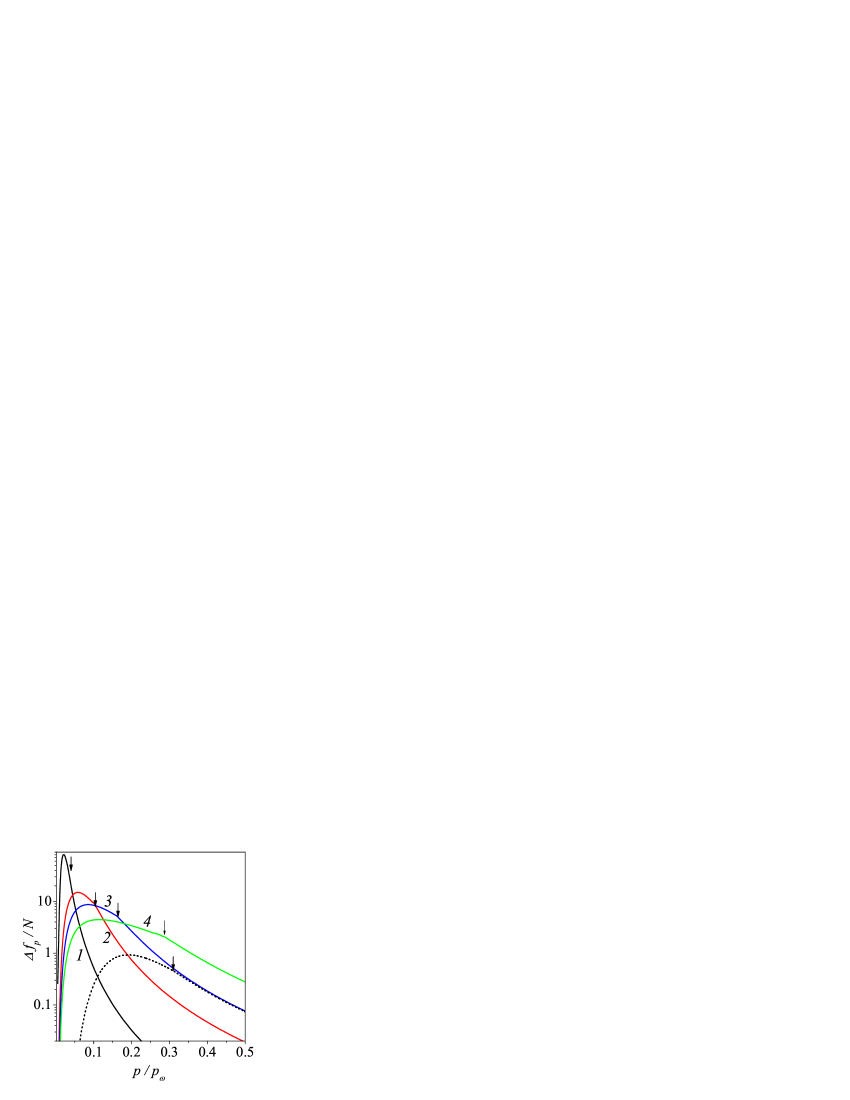
Figure 2: (Color online) Distribution function $\Delta f_{p}$ normalized to $N=\Delta f_{\omega}(p_{\omega}/p_{\scriptscriptstyle T})^{2}$ under 100 meV photoexcitation at $T=$4.2 K (1), 20 K (2), 40 K (3), and 77 K (4) and under 10 meV photoexcitation at $T=$4.2 K (dotted curve). The connection points $p_{c}/p_{\omega}$ are marked by arrows.

The distribution function $\Delta f_{p}$, which is normalized by the factor $N=\Delta f_{\omega}(p_{\omega}/p_{\scriptscriptstyle T})^{2}$ and calculated for different temperatures and $\hbar\omega=$ 100 meV, is shown in Fig. 2. This function calculated for $\hbar\omega=$ 10 meV at $T=$4.2 K is plotted as well. Due to fairly effective recombination at $p\sim p_{\scriptscriptstyle T}$, the distributions approach zero in the low-energy region. On the other hand, the fast decreasing distributions takes place at $p>p_{c}$. As a result, the main part of photoexcited carriers is localized in the region below $p_{c}$ and a peak of distribution grows up as $p_{\omega}/p_{\scriptscriptstyle T}$ increases. In order to find the conditions of the linear (with respect to $\nu_{\scriptscriptstyle E}$) response, we use $N\propto\omega^{-3}T^{-2}$ and set $\max(\Delta f_{p})\simeq 0.3$. Fig. 3 shows the region of parameters (in the ”pumping - temperature” plane at different $\hbar\omega$) where the linear response takes place. As seen, the threshold of nonlinear response dramatically decreases with decreasing of $\hbar\omega$ and $T$. For instance, the threshold is about 0.6 $\mu$W/cm² at $T=$4.2 K and 10 meV excitation.

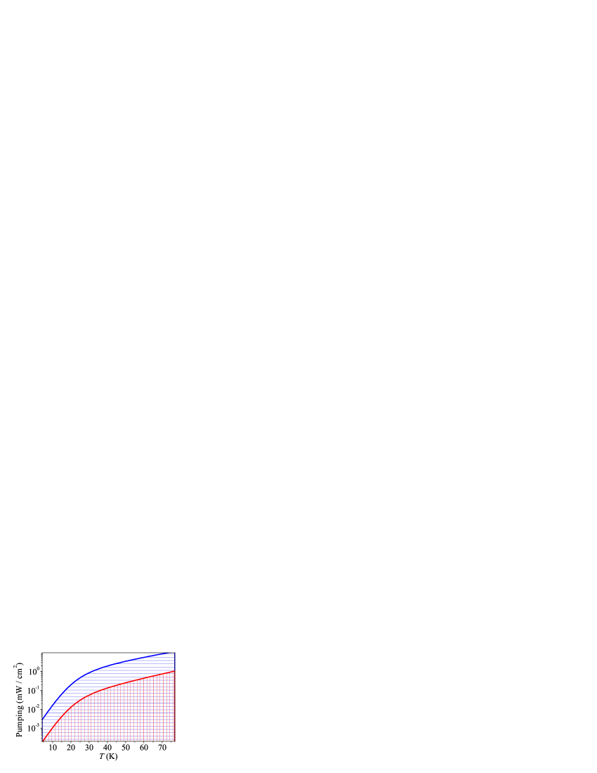
Figure 3: (Color online) Region of parameters (shaded by horisontal and vertical lines for $\hbar\omega=$ 100 meV and 40 meV, respectively) where the linear regime of response takes place.

IV Photoresponse

Finally, we consider the photoresponse by using Eq. (18) and distribution function (28). The contribution of the photoexcited carriers to the conductivity, $\Delta\sigma$, is given by the formula

$$\frac{\Delta\sigma}{\sigma_{eq}}=\Delta f_{\omega}\Psi\left(\frac{pl_{c}}{\hbar}\right)^{-1}+\frac{l_{c}}{\hbar}\int\limits_{0}^{p_{\omega}}dp\Delta f_{p}\Phi\left(\frac{pl_{c}}{\hbar}\right)$$

$$\simeq\left(\frac{2l_{c}}{\hbar}\right)^{2}\int\limits_{0}^{p_{c}}dpp\Delta f_{p}+\frac{l_{c}}{\hbar}\int\limits_{p_{c}}^{p_{\omega}}dp\Delta f_{p}\Phi\left(\frac{pl_{c}}{\hbar}\right),$$ (36)

where we have neglected $\propto\Delta f_{\omega}$ contribution in the lower expression. With the parameter $p_{\omega}l_{c}/\hbar=\hbar\omega/(2v_{\scriptscriptstyle W}\hbar/l_{c})$, which contains the characteristic energy $2v_{\scriptscriptstyle W}\hbar/l_{c}$=125 meV at $l_{c}=$10 nm, decreases, one can use the expansion $\Phi(z)\simeq 4z$. In this case Eq. (31) can be transformed into the following:

$$\frac{\Delta\sigma}{\sigma_{eq}}\simeq 2\pi l_{c}^{2}\Delta n.$$ (37)

Here $\Delta n=(4/L^{2})\sum_{\bf p}\Delta f_{p}$ is the photoexcited concentration of carriers which is given by

$$\Delta n\simeq\frac{2}{\pi\hbar^{2}}\int\limits_{0}^{p_{\omega}}dpp\Delta f_{p}.$$ (38)

Thus, the photoresponse can be calculated by using the substitution of Eq. (28) into Eq. (31) or (33) and numerical integration.

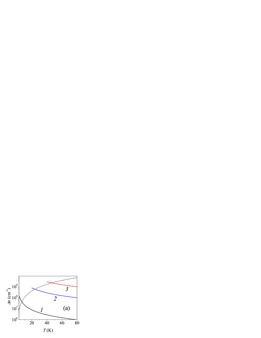
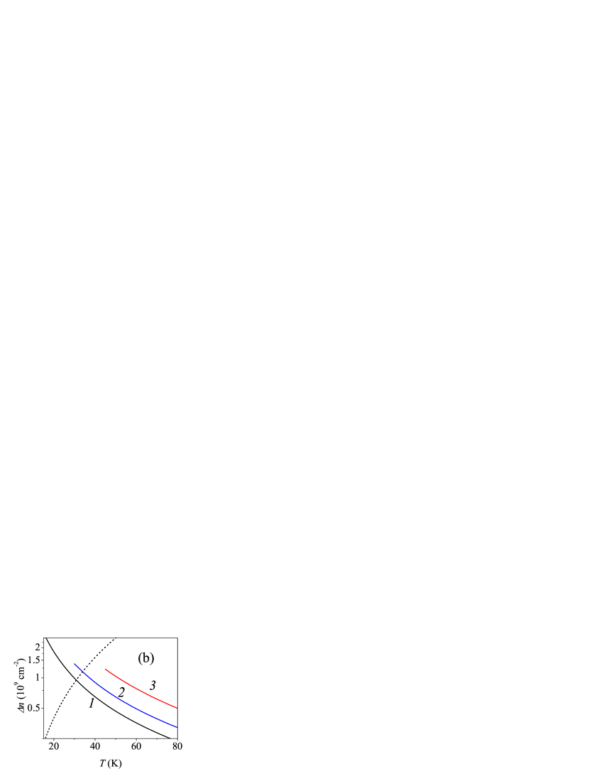
Figure 4: (Color online) Photoinduced concentration $\Delta n$ versus temperature: (a) for the pumping intensities 3 $\mu$W/cm² (1), 0.3 mW/cm² (2), and 3 mW/cm² (3) at $\hbar\omega$=100 meV and (b) for the excitation energies $\hbar\omega$=140 meV (1), 100 meV (2), and 60 meV (3) at the intensity 1 mW/cm². Dotted curve shows the equilibrium concentration.

Consider first the short-range scattering case, $p_{\omega}l_{c}/\hbar\ll 1$, which is described by the photoinduced concentration, $\Delta n$. The temperature dependencies of $\Delta n$, which are calculated for different intensities and different frequencies of excitation, are shown in Figs. 4(a) and 4(b), respectively. Curves 2 and 3 are plotted for the linear response region (see Fig. 3). The photoinduced concentration decreases with increasing $T$ and $\hbar\omega$, whereas it increases with pumping intensity. Fig. 5 presents the spectral dependencies of $\Delta n$ for different temperatures. Despite of $\Delta n$ exceeds (or be comparable with) the equilibrium concentration, $n_{eq}\simeq 0.52(T/\hbar v_{\scriptscriptstyle W})^{2}$, the relative photoconductivity (32) does not exceed 10^-2 for the short-range scattering case, when $l_{c}\leq$10 nm for the parameters used.

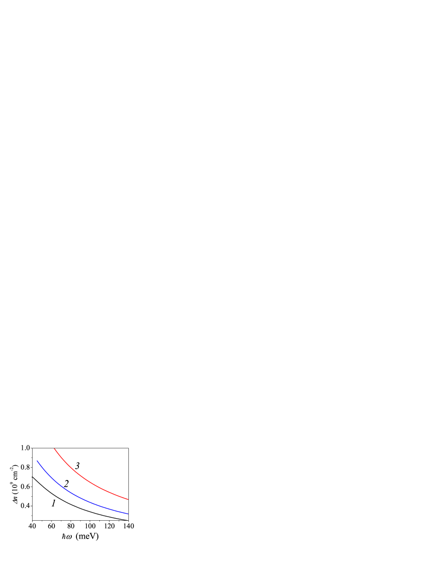
Figure 5: (Color online) Spectral dependencies of photoinduced concentration for $T$=50 K (1), 65 K (2), and 77 K (3) at the pumping intensity 1 mW/cm².

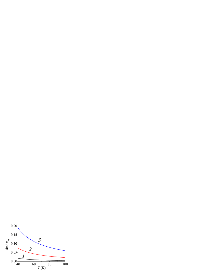
Figure 6: (Color online) Relative photoconductivity $\Delta\sigma/\sigma_{eq}$ vs temperature for different correlation lenths $l_{c}$=10 nm (1), 20 nm (2), and 30 nm (3) at the pumping intensity 3 mW/cm² and $\hbar\omega$=100 meV.

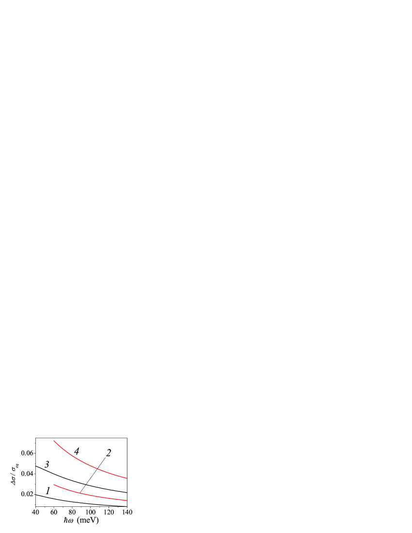
Figure 7: (Color online) Spectral dependencies of relative photoconductivity for the pumping intensity 1 mW/cm² and the correlation lengths $l_{c}$=20 nm at $T$=77 K (1) or $T$=50 K (2) and 20 nm at $T$=77 K (3) or $T$=50 K (4).

In the general case $p_{\omega}l_{c}/\hbar\sim 1$, which occurs if $l_{c}\geq$10 nm, by using Eqs. (28) and (31) we obtain $\Delta\sigma/\sigma_{eq}$ vs $T$ and $\hbar\omega$ relations as shown in Figs. 6 and 7, respectively. Once again the relative photoconductivity decreases with $T$ or $\hbar\omega$; these dependencies are similar to $\Delta n$ vs $T$ and $\hbar\omega$ but an additional dependency on $l_{c}$ becomes essential. In Fig. 7 (curves 2 and 3) we restrict ourselves by the linear response region. Since $\Delta\sigma/\sigma_{eq}$ increases with increasing of $l_{c}$ or intensity, for the above-discussed region of parameters one obtains $\Delta\sigma/\sigma_{eq}\sim$ 1.

For the case of far-IR excitation with the energy $\hbar\omega=$10 meV and intensity 1$\mu$W/cm², one obtains the photoinduced concentration $\Delta n\simeq 4.1\cdot 10^{7}$ cm^-2 at 4.2 K while the equilibrium concentration is about $1.7\cdot 10^{7}$ cm^-2. Since the short-range scattering condition is valid now up to $l_{c}\leq$30 nm, the relative photoconductivity $\Delta\sigma/\sigma_{eq}\propto l_{c}^{2}$ does not exceed 0.3 %.

V Concluding remarks

In the present work, we have considered the photoconductivity of intrinsic graphene under far- or mid-IR excitation of electron-hole pairs. We demonstrated that not only carrier concentration but also the energy distribution substantially depend on the parameters of excitation (frequency and pumping intensity) and the temperature. In contrast to the customary semiconductor materials, in which the recombination is a most slow process, interplay between recombination-generation and energy relaxation in graphene is crucial. The carrier distribution smeared up to the energy of photoexcitation can be realized due to a weak coupling to the phonon thermostat and effective radiative interband transitions.

In addition to the physical peculiarities presented, the technical results obtained might be useful for theoretical descriptions of the nonequilibrium carriers in graphene (heating under dc field, nonlinear optical properties, etc). We have evaluated the generation rate that describes the interband pumping of electron-hole pairs and described by the generation-recombination processes caused by the interaction of carriers with the thermal radiation. We also evaluated the Fokker-Planck collision integral governed the quasi-elastic energy relaxation due to the deformation interaction between carriers and acoustic phonons.

Let us briefly discuss the assumptions used in our treatment. The main restrictions arise from the low-concentration approximation, when one can neglect the intra- and interband Coulomb scattering. This approach corresponds to an intrinsic graphene at low temperatures which is sensitive to photoexcitation due to a high resistance. We also do not consider a disorder-induced channel of generation-recombination and restrict ourselves taking into account the simplest scattering mechanisms (elastic scattering by static disorder and deformation interaction with acoustic phonons). These restrictions are caused by the lack of data on relaxation process. However, the model used allows us to describe important peculiarities of photoresponse. Other assumptions are a rather standard for the calculations of the transport characteristics. We used the isotropic energy spectrum both for carriers and phonons, and consider the quasi-elastic electron-phonon scattering. We neglect an interaction with optical phonons because the optical phonon energy substantially exceeds $T$ and $\hbar\omega$. These restrictions are valid for low temperatures in the far- and mid-IR spectral regions.

Besides this, we restrict ourselves by the analytical consideration of the limiting case presented in Sec. III and do not perform a numerical solution of Eq. (19) with a subsequent integration of (18). This is because the lack of a precise data concerns both momentum relaxation (see the discussions in Refs. 4-6) and phonon scattering (see phonon and Refs. therein). Although the analytical consideration does not provide a complete qualitative description, the relations obtained permit one to estimate a character of photoresponse for the linear regime with arbitrary scattering parameters.

In closing, the obtained results demonstrated a marked photosensitivity of intrinsic graphene at low temperatures. This allows one to analyze the relaxation processes in graphene by using a photoconductivity data. In order to check a potential of graphene-based detector applications, one needs to perform a numerical modeling, including the nonlinear regime of response.

*

Appendix A Collision Integrals

Below we will evaluate the collision integrals used in Sec. II and our consideration is based on the general expression 7mono :

$$J\{F|\alpha\}=\sum_{\alpha^{\prime}}\left[{W_{\alpha^{\prime}\alpha}(1-F_{\alpha})F_{\alpha^{\prime}}-W_{\alpha\alpha^{\prime}}(1-F_{\alpha^{\prime}})F_{\alpha}}\right],$$ (39)

where $F_{\alpha}$ is the distribution function over $\alpha$-state. The transition probabilities, $W_{\alpha\alpha^{\prime}}$, are connected by the detailed balance requirement: $W_{\alpha^{\prime}\alpha}=\exp[-(\varepsilon_{\alpha}-\varepsilon_{\alpha^{\prime}})/T]$ $\times W_{\alpha\alpha^{\prime}}$ and are determined through

$$W_{\alpha\alpha^{\prime}}=\frac{2\pi}{\hbar}\sum_{q}|\langle\alpha^{\prime}|\hat{\chi}_{q}|\alpha\rangle|^{2}~{}~{}~{}~{}~{}~{}$$ (40)

$$\times\left[{(N_{q}+1)\delta(\varepsilon_{\alpha}-\varepsilon_{\alpha}-\hbar\omega_{q})+N_{q}\delta(\varepsilon_{\alpha}-\varepsilon_{\alpha}+\hbar\omega_{q})}\right].$$

Here $N_{q}$ is the Planck distribution of the $q$th boson (phonon or photon) mode of frequency $\omega_{q}$ and the matrix element $\langle\alpha^{\prime}|\hat{\chi}_{q}|\alpha\rangle$ describes the electron-boson interaction.

A.1 Radiative-induced transitions

First, we consider the interaction with thermal radiation when the secondary-quantized radiation field should be substituted into perturbation operator (2) (see Secs. 20 and 38 in 7mono ). As a result, the operator $\hat{\chi}_{q}$ in (A.2) takes the form:

$$\hat{\chi}_{\eta,{\scriptscriptstyle{\bf Q}}}=v_{\scriptscriptstyle W}\sqrt{\frac{2\pi\hbar e^{2}}{\omega_{\scriptscriptstyle Q}\epsilon V}}\left(\hat{\mbox{\boldmath$\sigma$}}\cdot{\bf e}_{\eta,{\scriptscriptstyle{\bf Q}}}\right),$$ (41)

where $V$ is the normalization volume, $\omega_{\scriptscriptstyle Q}$ and ${\bf e}_{\eta,{\scriptscriptstyle{\bf Q}}}$ are the frequency and the polarization vector of the photon mode with the 3D wave vector $\bf Q$ and the polarization $\eta$. We have also neglected in (A3) the in-plane momentum transfer under interband transitions. Calculations of the matrix elements (A.3) are performed similar to Sec. IIA 9eg and we obtain

$$|\left\langle{\pm 1,{\bf p}}\right|\hat{\chi}_{\eta,{\scriptscriptstyle{\bf Q}}}\left|{\mp 1,{\bf p}}\right\rangle|^{2}=v_{\scriptscriptstyle W}^{2}\frac{{\pi\hbar e^{2}}}{{\omega_{\scriptscriptstyle Q}\epsilon V}}|{\bf e}_{\eta,{\scriptscriptstyle{\bf Q}}}^{\scriptscriptstyle\|}|^{2}$$ (42)

while the intraband transitions are forbidden. The averaging over polarization and direction of photons gives $\overline{|{\bf e}_{\eta,{\scriptscriptstyle{\bf Q}}}^{\scriptscriptstyle\|}|^{2}}=2/3$.

After substituting Eq. (A.4) to general expression (A.2), we obtain the interband probabilities:

$$\left|{\begin{array}[]{*{20}c}{W_{+1p,-1p}}\\ {W_{-1p,+1p}}\\ \end{array}}\right|=\frac{2(2\pi ev_{\scriptscriptstyle W})^{2}}{3\epsilon}\int\frac{d{\bf Q}}{(2\pi)^{3}}\omega_{\scriptscriptstyle Q}^{-1}$$ (45)

$$\times\left|{\begin{array}[]{*{20}c}{N_{\scriptscriptstyle Q}+1}\\ N_{\scriptscriptstyle Q}\\ \end{array}}\right|\delta(2v_{\scriptscriptstyle W}p-\hbar\omega_{\scriptscriptstyle Q})$$ (48)

where $N_{\scriptscriptstyle Q}$ stands for the Planck number of photons with temperature $T$. Taking the integral over $\bf Q$-space we obtain

$$\left|{\begin{array}[]{*{20}c}{W_{+1p,-1p}}\\ {W_{-1p,+1p}}\\ \end{array}}\right|=\nu_{p}^{\scriptscriptstyle(R)}\left|{\begin{array}[]{l}N_{2p/p_{\scriptscriptstyle T}}+1\\ ~{}~{}~{}~{}~{}N_{2p/p_{\scriptscriptstyle T}}\\ \end{array}}\right|,$$ (49)

where the rate $\nu_{p}^{\scriptscriptstyle(R)}$ is given by Eq. (10).

By using (A.6), one can transform collision integral (A.1) as follows

$$J_{\scriptscriptstyle R}\{f|\pm 1,p\}=\nu_{p}^{\scriptscriptstyle(\mp)}(1-F_{\pm 1,p})F_{\mp 1,p}-\nu_{p}^{\scriptscriptstyle(\pm)}(1-F_{\mp 1,p})F_{\pm 1,p},$$ (50)

where the rates of generation ($\nu_{p}^{\scriptscriptstyle(+)}$) and recombination ($\nu_{p}^{\scriptscriptstyle(-)}$) are given by Eq. (9). We further use the electron-hole representation introduced by Eq. (5) and the radiative collision integral for electrons takes the form:

$$J_{\scriptscriptstyle R}\{f|ep\}=\nu_{p}^{\scriptscriptstyle(-)}(1-f_{ep})(1-f_{hp})-\nu_{p}^{\scriptscriptstyle(+)}f_{ep}f_{hp}$$ (51)

and $J_{\scriptscriptstyle R}\{f|hp\}=-J_{\scriptscriptstyle R}\{f|ep\}$, which are in agreement with the particle conservation law. Here the recombination term is proportional to $f_{ep}f_{hp}$, while the generation contribution is proportional to $(1-f_{ep})(1-f_{hp})$, also $\nu_{p}^{\scriptscriptstyle(+)}$ and $\nu_{p}^{\scriptscriptstyle(-)}$ mean the rates of spontaneous emission and absorption.

A.2 Acoustic phonon scattering

We further consider the collision integral that is described the intraband transitions caused by the acoustic phonon scattering while the interband transitions are forbidden due to the condition $s\ll v_{\scriptscriptstyle W}$. The main contribution to the acoustic phonon scattering appears due to the deformation interaction with longitudinal vibrations ando , $D\nabla\cdot{\bf u}_{\bf x}$, where ${\bf u}_{\bf x}$ is the displacement vector of LA-mode. By using the quantized displacement operator, one obtains the matrix element of Eq. (A.2) in the standard form 10 :

$$\left|\left\langle l^{\prime}{\bf p}^{\prime}|\hat{\chi}_{\bf q}|l{\bf p}\right\rangle\right|^{2}\simeq\delta_{{\bf p}^{\prime},{\bf p}+\hbar{\bf q}}|C_{|{\bf p}-{\bf p^{\prime}}|/\hbar}|^{2}\Psi\left(\widehat{{\bf p^{\prime}},{\bf p}}\right)$$ (52)

Here, $\bf q$ is the 2D wave vector of phonon with frequency $\omega_{q}=sq$ and $|C_{q}|^{2}=D^{2}\hbar\omega_{q}/(2\rho_{s}s^{2}L^{2})$ stands as the electron-phonon matrix element. The overlap factor, $\Psi\left(\widehat{{\bf p^{\prime}},{\bf p}}\right)$, is given by 9eg :

$$\Psi\left(\widehat{{\bf p^{\prime}},{\bf p}}\right)\equiv\left|\left\langle l{\bf p}^{\prime}|l{\bf p}\right\rangle\right|^{2}=\frac{1+\cos\widehat{{\bf p^{\prime}},{\bf p}}}{2}.$$ (53)

Since (A.9) does not depend on $l=\pm 1$ (electron-hole symmetry), we obtain $W_{+1{\bf p},+1{\bf p}^{\prime}}=W_{-1{\bf p},-1{\bf p^{\prime}}}=W_{\bf pp^{\prime}}$ and the transition probability is given by

$$W_{\bf pp^{\prime}}=\frac{2\pi}{\hbar}\Psi(\widehat{{\bf p},{\bf p^{\prime}}})\left|{C_{|{\bf p}-{\bf p}^{\prime}|/\hbar}}\right|^{2}~{}~{}~{}~{}~{}$$ (54)

$$\times\left\{(N_{|{\bf p}-{\bf p^{\prime}}|/\hbar}+1)\delta[v{\scriptscriptstyle W}(p-p^{\prime})-s|{\bf p}-{\bf p}^{\prime}|]\right.$$

$$\left.+N_{|{\bf p}-{\bf p}^{\prime}|/\hbar}\delta[v_{\scriptscriptstyle W}(p-p^{\prime})+s|{\bf p}-{\bf p}^{\prime}|]\right\},$$

where $N_{q}$ is the Planck distribution of phonons with temperature $T$. By using the electron-hole representation, see Eq. (5), one transforms collision integral (A.1) into the form:

$$J_{\scriptscriptstyle LA}\{f|k{\bf p}\}=\sum_{\bf p^{\prime}}\left[W_{\bf p^{\prime}p}(1-f_{k{\bf p}})f_{k{\bf p^{\prime}}}\right.$$

$$\left.-W_{\bf pp^{\prime}}(1-f_{k{\bf p^{\prime}}})f_{k{\bf p}}\right],$$ (55)

with transition probabilities (A.11) that are the same for electrons ($k=e$) and holes ($k=h$).

References

- (1) A.K. Geim and A.H. MacDonald, Physics Today 60, 35 (2006); A.H. Castro Neto, F. Guinea, N.M.R. Peres, K.S. Novoselov, and A.K. Geim, arXiv:0709.1163.
- (2) A.K. Geim and K.S. Novoselov, Nature Materials 6, 183 (2007); M.I. Katsnelson, K.S. Novoselov, A.K. Geim. Nature Phys. 2 620 (2006); M.I. Katsnelson, Materials Today 10, 20 (2007).
- (3) E.M. Lifshitz, L.P. Pitaevskii, and V.B. Berestetskii, Quantum Electrodynamics, (Butterworth-Heinemann, Oxford 1982); P.R. Wallace, Phys. Rev. 71, 622 (1947).
- (4) K.S. Novoselov, A.K. Geim, S.V. Morozov, D. Jiang, Y. Zhang, S.V. Dubonos, I.V. Grigorieva, A.A. Firsov, Science, 306 666 (2004); Y. Zhang, Y.-W. Tan, H.L. Stormer, and P. Kim, Nature 438, 201 (2005); Y.-W. Tan, Y. Zhang, H.L. Stormer, and P. Kim, Eur. Phys. J. Special Topics 148, 15 (2007); E.W. Hill, A.K. Geim, K. Novoselov, F. Schedin and P. Blake, IEEE Trans. Magn. 42, 2694 (2006); Y. -W. Tan, Y. Zhang, K. Bolotin, Y. Zhao, S. Adam, E. H. Hwang, S. Das Sarma, H. L. Stormer, P. Kim, arXiv:0707.1807;
- (5) T. Ando, J. Phys. Soc. Japan, 75, 074716 (2006); L.A. Falkovsky, Phys. Rev. B 75 033409 (2007); M.I. Katsnelson and A.K. Geim, arXiv:0706.2490. T. Stauber, N.M.R. Peres, and F. Guinea, Phys. Rev. B 76, 205423 (2007); N.M.R. Peres, J.M.B. Lopes dos Santos, and T. Stauber, Phys. Rev. B 76, 073412 (2007); E.H. Hwang, S. Adam, and S. Das Sarma,Phys. Rev. Lett. 98, 186806 (2007).
- (6) F.T. Vasko and V. Ryzhii, Phys. Rev. B 76, 233404 (2007).
- (7) S. Butscher, F. Milde, M. Hirtschulz, E. Malic, and A. Knorr, Appl. Phys. Lett. 91, 203103 (2007).
- (8) F.T. Vasko and O.E. Raichev, Quantum Kinetic Theory and Applications (Springer, N.Y. 2005).
- (9) One can estimate the broadening , so that .
-
(10)
Under calculations of the matrix elements of in Eqs. (3), (A.4) and the
overlap factor (A.10) we used the solution of the eigenstate problem given by by the dispersion laws
with and the eigenvectors:
where is the -plane polar angle. - (11) A.I. Anselm, Introduction to Semiconductor Theory (Prentice-Hall, Englewood Cliffs, NJ, 1981).
- (12) E.M. Lifshitz and L.P. Pitaevskii, Physical Kinetics (Pergamon Press, Oxford, 1981).
- (13) F.W.J. Olver, Asymptotics and Special Functions (Academic Press, N.Y.,1974).
- (14) The low-temperature restriction on the consideration performed appears due to the quasielastic approach in the transition probabilities (12) and results in the condition which is valid for 4 K if 100 meV.
- (15) H. Suzuura and T. Ando, Phys. Rev. B 65, 235412 (2002).
- (16) S. V. Morozov, K.S. Novoselov, M.I. Katsnelson, F. Schedin, D. Elias, J.A. Jaszczak, and A.K. Geim arXiv:0710.5304; E. H. Hwang and S. Das Sarma, arXiv:0711.0754.