Abstract
Diffusion-induced Ramsey narrowing that appears when atoms can leave the interaction region and repeatedly return without lost of coherence is investigated using strong collisions approximation. The effective diffusion equation is obtained and solved for low-dimensional model configurations and three-dimensional real one.
II Basic Equations
In the classical problem of migration of a particle in the gas
the kinetic equation for the distribution function ρ ( t → , v → , t ) 𝜌 → 𝑡 → 𝑣 𝑡 \rho(\vec{t},\vec{v},t) Rautian and Sobelman (1966 ) , Rautian (1991 ) ):
∂ ρ ∂ t + ( v → ⋅ ∇ → ) ρ = 𝒮 , 𝜌 𝑡 ⋅ → 𝑣 → ∇ 𝜌 𝒮 \frac{\partial\rho}{\partial t}+(\vec{v}\cdot\vec{\nabla})\rho=\,\mathcal{S}\,, (1)
where 𝒮 𝒮 \,\mathcal{S} ρ 𝜌 \rho
𝒮 = − ∫ [ 𝒜 ( v → , v → ′ ) ρ ( r → , v → , t ) − 𝒜 ( v → ′ , v → ) ρ ( r → , v → ′ , t ) ] 𝑑 v → ′ . 𝒮 delimited-[] 𝒜 → 𝑣 superscript → 𝑣 ′ 𝜌 → 𝑟 → 𝑣 𝑡 𝒜 superscript → 𝑣 ′ → 𝑣 𝜌 → 𝑟 superscript → 𝑣 ′ 𝑡 differential-d superscript → 𝑣 ′ \,\mathcal{S}=-\int\bigl{[}\,\mathcal{A}(\vec{v},\vec{v}^{\prime})\rho(\vec{r},\vec{v},t)-\,\mathcal{A}(\vec{v}^{\prime},\vec{v})\rho(\vec{r},\vec{v}^{\prime},t)\bigr{]}\,d\vec{v}^{\prime}\,. (2)
Here 𝒜 ( v → , v → ′ ) 𝒜 → 𝑣 superscript → 𝑣 ′ \,\mathcal{A}(\vec{v},\vec{v}^{\prime}) v → → v → ′ → → 𝑣 superscript → 𝑣 ′ \vec{v}\to\vec{v}^{\prime} ρ ( r → , v → , 0 ) = W ( v → ) δ ( r → ) 𝜌 → 𝑟 → 𝑣 0 𝑊 → 𝑣 𝛿 → 𝑟 \rho(\vec{r},\vec{v},0)=W(\vec{v})\delta(\vec{r}) W ( v → ) 𝑊 → 𝑣 W(\vec{v})
The collision integral can be written as
𝒮 = − ν ρ ( r → , v → , t ) + ∫ [ − 𝒜 ( v → ′ , v → ) ρ ( r → , v → ′ , t ) ] 𝑑 v → ′ , 𝒮 𝜈 𝜌 → 𝑟 → 𝑣 𝑡 delimited-[] 𝒜 superscript → 𝑣 ′ → 𝑣 𝜌 → 𝑟 superscript → 𝑣 ′ 𝑡 differential-d superscript → 𝑣 ′ \,\mathcal{S}=-\nu\rho(\vec{r},\vec{v},t)+\int\bigl{[}-\,\mathcal{A}(\vec{v}^{\prime},\vec{v})\rho(\vec{r},\vec{v}^{\prime},t)\bigr{]}\,d\vec{v}^{\prime}\,, (3)
where
ν ( v → ) = ∫ 𝒜 ( v → , v → ′ ) 𝑑 v → ′ 𝜈 → 𝑣 𝒜 → 𝑣 superscript → 𝑣 ′ differential-d superscript → 𝑣 ′ \nu(\vec{v})=\int\,\mathcal{A}(\vec{v},\vec{v}^{\prime})\,d\vec{v}^{\prime} (4)
denote the effective collision frequency.
There are two simple models that allow one to investigate the kinetic equation (1 3 ρ 𝜌 \rho
The second model based on the approximation of strong collisions
(light atoms scatter on heavy particles). In this model the function 𝒜 ( v → ′ , v → ) 𝒜 superscript → 𝑣 ′ → 𝑣 \,\mathcal{A}(\vec{v}^{\prime},\vec{v}) v → ′ superscript → 𝑣 ′ \vec{v}^{\prime} v → → 𝑣 \vec{v} 𝒜 ( v → ) 𝒜 → 𝑣 \,\mathcal{A}(\vec{v}) 𝒮 = 0 𝒮 0 \,\mathcal{S}=0 ν = const 𝜈 const \nu=\,\mathrm{const}
𝒜 ( v → ) = ν W ( v → ) . 𝒜 → 𝑣 𝜈 𝑊 → 𝑣 \,\mathcal{A}(\vec{v})=\nu W(\vec{v})\,.
This expression means that an arbitrary initial distribution turn to Maxwell
after the lapse of time 1 / ν 1 𝜈 1/\nu 1 / ν 1 𝜈 1/\nu
Finally, the kinetic equation for the problem of migration of the atom in gas
in approximation of strong collisions has the form:
∂ ρ ∂ t + ( v → ⋅ ∇ → ) ρ = − ν ρ + ν W ( v → ) ∫ ρ ( r → , v → , t ) 𝑑 v → . 𝜌 𝑡 ⋅ → 𝑣 → ∇ 𝜌 𝜈 𝜌 𝜈 𝑊 → 𝑣 𝜌 → 𝑟 → 𝑣 𝑡 differential-d → 𝑣 \frac{\partial\rho}{\partial t}+(\vec{v}\cdot\vec{\nabla})\rho=-\nu\rho+\nu W(\vec{v})\int\rho(\vec{r},\vec{v},t)\,d\vec{v}\,.
The same approach can be used (see Rautian (1991 ) ) for non-diagonal elements of density matrix.
For two-level system we have:
∂ ρ 12 ∂ t + ( v → ⋅ ∇ → ) ρ 12 = − ( ν + γ + i Δ ω ) ρ 12 + ν W ( v → ) ∫ ρ 12 ( r → , v → , t ) 𝑑 v → + q ( r → , v → ) , subscript 𝜌 12 𝑡 ⋅ → 𝑣 → ∇ subscript 𝜌 12 𝜈 𝛾 𝑖 Δ 𝜔 subscript 𝜌 12 𝜈 𝑊 → 𝑣 subscript 𝜌 12 → 𝑟 → 𝑣 𝑡 differential-d → 𝑣 𝑞 → 𝑟 → 𝑣 \frac{\partial\rho_{12}}{\partial t}+(\vec{v}\cdot\vec{\nabla})\rho_{12}=-(\nu+\gamma+i\Delta\omega)\rho_{12}+\nu W(\vec{v})\int\rho_{12}(\vec{r},\vec{v},t)\,d\vec{v}+q(\vec{r},\vec{v})\,,
where γ 𝛾 \gamma q ( r → , v → ) 𝑞 → 𝑟 → 𝑣 q(\vec{r},\vec{v}) Δ ω Δ 𝜔 \Delta\omega
We will consider the stationary case.
Denoting ρ ( r → , v → ) = ρ 12 ( r → , v → ) 𝜌 → 𝑟 → 𝑣 subscript 𝜌 12 → 𝑟 → 𝑣 \rho(\vec{r},\vec{v})=\rho_{12}(\vec{r},\vec{v})
( v → ⋅ ∇ → ) ρ ( r → , v → ) = − ( ν + γ + i Δ ω ) ρ ( r → , v → ) + W ( v → ) [ λ ( r → ) + ν ∫ 𝑑 v → ρ ( r → , v → ) ] , ⋅ → 𝑣 → ∇ 𝜌 → 𝑟 → 𝑣 𝜈 𝛾 𝑖 Δ 𝜔 𝜌 → 𝑟 → 𝑣 𝑊 → 𝑣 delimited-[] 𝜆 → 𝑟 𝜈 differential-d → 𝑣 𝜌 → 𝑟 → 𝑣 (\vec{v}\cdot\vec{\nabla})\rho(\vec{r},\vec{v})=-(\nu+\gamma+i\Delta\omega)\rho(\vec{r},\vec{v})+W(\vec{v})\left[\lambda(\vec{r})+\nu\int d\vec{v}\,\rho(\vec{r},\vec{v})\right]\,, (5)
where
W ( v → ) = W 0 e − v → 2 / v 0 2 , λ ( r → ) = λ 0 e − r → 2 / a 2 . formulae-sequence 𝑊 → 𝑣 subscript 𝑊 0 superscript 𝑒 superscript → 𝑣 2 superscript subscript 𝑣 0 2 𝜆 → 𝑟 subscript 𝜆 0 superscript 𝑒 superscript → 𝑟 2 superscript 𝑎 2 W(\vec{v})=W_{0}e^{-\vec{v}\,^{2}/v_{0}^{2}}\,,\quad\lambda(\vec{r})=\lambda_{0}e^{-\vec{r}\,^{2}/a^{2}}\,.
and W 0 subscript 𝑊 0 W_{0}
Let us denote
N ( r → ) = ∫ 𝑑 v → ρ ( r → , v → ) , α = ν + γ + i Δ ω , α 0 = γ + i Δ ω . formulae-sequence 𝑁 → 𝑟 differential-d → 𝑣 𝜌 → 𝑟 → 𝑣 formulae-sequence 𝛼 𝜈 𝛾 𝑖 Δ 𝜔 subscript 𝛼 0 𝛾 𝑖 Δ 𝜔 N(\vec{r})=\int d\vec{v}\,\rho(\vec{r},\vec{v})\,,\quad\alpha=\nu+\gamma+i\Delta\omega\,,\quad\alpha_{0}=\gamma+i\Delta\omega\,.
The complex signal is defined as:
𝖲 ( Δ ω ) = ∬ 𝑑 r → 𝑑 v → λ ( r → ) ρ ( r → , v → ) = ∫ N ( r → ) λ ( r → ) 𝑑 r → . 𝖲 Δ 𝜔 double-integral differential-d → 𝑟 differential-d → 𝑣 𝜆 → 𝑟 𝜌 → 𝑟 → 𝑣 𝑁 → 𝑟 𝜆 → 𝑟 differential-d → 𝑟 \,\mathsf{S}(\Delta\omega)=\iint d\vec{r}\,d\vec{v}\,\lambda(\vec{r})\rho(\vec{r},\vec{v})=\int N(\vec{r})\lambda(\vec{r})\,d\vec{r}\,. (6)
We assume that
Δ ω , γ ≪ ν , ν ≫ v 0 a = 1 τ 0 , formulae-sequence much-less-than Δ 𝜔 𝛾
𝜈 much-greater-than 𝜈 subscript 𝑣 0 𝑎 1 subscript 𝜏 0 \Delta\omega,\gamma\ll\nu\,,\quad\nu\gg\frac{v_{0}}{a}=\frac{1}{\tau_{0}}\,,
where τ a = a v 0 subscript 𝜏 𝑎 𝑎 subscript 𝑣 0 \tau_{a}=\frac{a}{v_{0}} τ a ≫ τ ν = 1 ν much-greater-than subscript 𝜏 𝑎 subscript 𝜏 𝜈 1 𝜈 \tau_{a}\gg\tau_{\nu}=\frac{1}{\nu}
For the atomic ensemble the atomic resonance line shape is determined by weighted average
of the line shapes from different Ramsey sequences (with alternating interactions with the laser beam and motion in the dark).
III Effective Diffusion Equation
According to (II 𝖲 ( Δ ω ) 𝖲 Δ 𝜔 \,\mathsf{S}(\Delta\omega) N ( r → ) 𝑁 → 𝑟 N(\vec{r}) ρ ( r → ) 𝜌 → 𝑟 \rho(\vec{r}) v → → 𝑣 \vec{v} N ( k ) ( r → ) superscript 𝑁 𝑘 → 𝑟 N^{(k)}(\vec{r})
N ( k ) ( x ) = ∫ − ∞ ∞ v k ρ ( x , v ) 𝑑 v , N ( 0 ) ( x ) = N ( x ) . formulae-sequence superscript 𝑁 𝑘 𝑥 superscript subscript superscript 𝑣 𝑘 𝜌 𝑥 𝑣 differential-d 𝑣 superscript 𝑁 0 𝑥 𝑁 𝑥 N^{(k)}(x)=\int\limits_{-\infty}^{\infty}v^{k}\rho(x,v)\,dv\,,\quad N^{(0)}(x)=N(x)\,.
Multiplying the equation
v ∂ ∂ x ρ ( x , v ) = − α ρ ( x , v ) + W ( v ) [ λ ( x ) + ν N ( 0 ) ( x ) ] 𝑣 𝑥 𝜌 𝑥 𝑣 𝛼 𝜌 𝑥 𝑣 𝑊 𝑣 delimited-[] 𝜆 𝑥 𝜈 superscript 𝑁 0 𝑥 v\frac{\partial}{\partial x}\rho(x,v)=-\alpha\rho(x,v)+W(v)\bigl{[}\lambda(x)+\nu N^{(0)}(x)\bigr{]}
by v k superscript 𝑣 𝑘 v^{k} v 𝑣 v
d N ( k + 1 ) d x = − α N ( k ) ( x ) + ⟨ v k ⟩ [ λ ( x ) + ν N ( 0 ) ( x ) ] , ⟨ v k ⟩ = ∫ − ∞ ∞ v k W ( v ) 𝑑 v . formulae-sequence 𝑑 superscript 𝑁 𝑘 1 𝑑 𝑥 𝛼 superscript 𝑁 𝑘 𝑥 delimited-⟨⟩ superscript 𝑣 𝑘 delimited-[] 𝜆 𝑥 𝜈 superscript 𝑁 0 𝑥 delimited-⟨⟩ superscript 𝑣 𝑘 superscript subscript superscript 𝑣 𝑘 𝑊 𝑣 differential-d 𝑣 \frac{dN^{(k+1)}}{dx}=-\alpha N^{(k)}(x)+\langle v^{k}\rangle\bigl{[}\lambda(x)+\nu N^{(0)}(x)\bigr{]}\,,\quad\langle v^{k}\rangle=\int\limits_{-\infty}^{\infty}v^{k}W(v)\,dv\,.
Since ⟨ v k ⟩ = 0 delimited-⟨⟩ superscript 𝑣 𝑘 0 \langle v^{k}\rangle=0 k 𝑘 k
d N ( 2 k + 1 ) d x = − α N ( 2 k ) + ⟨ v 2 k ⟩ [ λ ( x ) + ν N ( 0 ) ( x ) ] , d N ( 2 k + 2 ) d x = − α N ( 2 k + 1 ) formulae-sequence 𝑑 superscript 𝑁 2 𝑘 1 𝑑 𝑥 𝛼 superscript 𝑁 2 𝑘 delimited-⟨⟩ superscript 𝑣 2 𝑘 delimited-[] 𝜆 𝑥 𝜈 superscript 𝑁 0 𝑥 𝑑 superscript 𝑁 2 𝑘 2 𝑑 𝑥 𝛼 superscript 𝑁 2 𝑘 1 \frac{dN^{(2k+1)}}{dx}=-\alpha N^{(2k)}+\langle v^{2k}\rangle\bigl{[}\lambda(x)+\nu N^{(0)}(x)\bigr{]}\,,\\
\quad\frac{dN^{(2k+2)}}{dx}=-\alpha N^{(2k+1)}
or, equivalently equations for even orders only:
1 α d 2 N ( 2 k + 2 ) d x 2 = α N ( 2 k ) − ⟨ v 2 k ⟩ [ λ ( x ) + ν N ( 0 ) ( x ) ] , 1 𝛼 superscript 𝑑 2 superscript 𝑁 2 𝑘 2 𝑑 superscript 𝑥 2 𝛼 superscript 𝑁 2 𝑘 delimited-⟨⟩ superscript 𝑣 2 𝑘 delimited-[] 𝜆 𝑥 𝜈 superscript 𝑁 0 𝑥 \frac{1}{\alpha}\frac{d^{2}N^{(2k+2)}}{dx^{2}}=\alpha N^{(2k)}-\langle v^{2k}\rangle\bigl{[}\lambda(x)+\nu N^{(0)}(x)\bigr{]}\,,\\
(7)
In these sequence of equations one can substitute the next equation to the previous and obtain the expression like the following:
α N ( 0 ) − [ λ ( x ) + ν N ( 0 ) ( x ) ] = 1 α d 2 N ( 2 ) d x 2 = ⟨ v 2 ⟩ α 2 d 2 d x 2 [ λ ( x ) + ν N ( 0 ) ( x ) ] + 1 α 3 d 4 N ( 4 ) d x 4 = … 𝛼 superscript 𝑁 0 delimited-[] 𝜆 𝑥 𝜈 superscript 𝑁 0 𝑥 1 𝛼 superscript 𝑑 2 superscript 𝑁 2 𝑑 superscript 𝑥 2 delimited-⟨⟩ superscript 𝑣 2 superscript 𝛼 2 superscript 𝑑 2 𝑑 superscript 𝑥 2 delimited-[] 𝜆 𝑥 𝜈 superscript 𝑁 0 𝑥 1 superscript 𝛼 3 superscript 𝑑 4 superscript 𝑁 4 𝑑 superscript 𝑥 4 … \alpha N^{(0)}-\bigl{[}\lambda(x)+\nu N^{(0)}(x)\bigr{]}=\frac{1}{\alpha}\frac{d^{2}N^{(2)}}{dx^{2}}=\frac{\langle v^{2}\rangle}{\alpha^{2}}\frac{d^{2}}{dx^{2}}\bigl{[}\lambda(x)+\nu N^{(0)}(x)\bigr{]}+\frac{1}{\alpha^{3}}\frac{d^{4}N^{(4)}}{dx^{4}}=\dots (8)
Performing the substitution k 𝑘 k
α N ( 0 ) = ( 1 + ⟨ v 2 ⟩ α 2 d 2 d x 2 + ⋯ + ⟨ v 2 k ⟩ α 2 k d 2 k d x 2 k ) [ λ ( x ) + ν N ( 0 ) ( x ) ] + 1 α 2 k + 1 d 2 k + 2 N ( 2 k + 2 ) d x 2 k + 2 . 𝛼 superscript 𝑁 0 1 delimited-⟨⟩ superscript 𝑣 2 superscript 𝛼 2 superscript 𝑑 2 𝑑 superscript 𝑥 2 ⋯ delimited-⟨⟩ superscript 𝑣 2 𝑘 superscript 𝛼 2 𝑘 superscript 𝑑 2 𝑘 𝑑 superscript 𝑥 2 𝑘 delimited-[] 𝜆 𝑥 𝜈 superscript 𝑁 0 𝑥 1 superscript 𝛼 2 𝑘 1 superscript 𝑑 2 𝑘 2 superscript 𝑁 2 𝑘 2 𝑑 superscript 𝑥 2 𝑘 2 \alpha N^{(0)}=\left(1+\frac{\langle v^{2}\rangle}{\alpha^{2}}\frac{d^{2}}{dx^{2}}+\dots+\frac{\langle v^{2k}\rangle}{\alpha^{2k}}\frac{d^{2k}}{dx^{2k}}\right)\bigl{[}\lambda(x)+\nu N^{(0)}(x)\bigr{]}+\frac{1}{\alpha^{2k+1}}\frac{d^{2k+2}N^{(2k+2)}}{dx^{2k+2}}\,.
For k → ∞ → 𝑘 k\to\infty
α N ( 0 ) = ∑ k = 0 ∞ ⟨ v 2 k ⟩ α 2 k d 2 k d x 2 k [ λ ( x ) + ν N ( 0 ) ( x ) ] = 𝖥 ^ [ λ ( x ) + ν N ( 0 ) ( x ) ] , 𝛼 superscript 𝑁 0 superscript subscript 𝑘 0 delimited-⟨⟩ superscript 𝑣 2 𝑘 superscript 𝛼 2 𝑘 superscript 𝑑 2 𝑘 𝑑 superscript 𝑥 2 𝑘 delimited-[] 𝜆 𝑥 𝜈 superscript 𝑁 0 𝑥 ^ 𝖥 delimited-[] 𝜆 𝑥 𝜈 superscript 𝑁 0 𝑥 \alpha N^{(0)}=\sum\limits_{k=0}^{\infty}\frac{\langle v^{2k}\rangle}{\alpha^{2k}}\frac{d^{2k}}{dx^{2k}}\bigl{[}\lambda(x)+\nu N^{(0)}(x)\bigr{]}=\hat{\,\mathsf{F}}\bigl{[}\lambda(x)+\nu N^{(0)}(x)\bigr{]}\,, (9)
where 𝖥 ^ ^ 𝖥 \hat{\,\mathsf{F}}
𝖥 ^ = ∫ − ∞ ∞ 𝑑 v W ( v ) ( 1 − v α d d x ) − 1 ^ 𝖥 superscript subscript differential-d 𝑣 𝑊 𝑣 superscript 1 𝑣 𝛼 𝑑 𝑑 𝑥 1 \hat{\,\mathsf{F}}=\int\limits_{-\infty}^{\infty}dv\,W(v)\biggl{(}1-\frac{v}{\alpha}\frac{d}{dx}\biggr{)}^{-1}
For higher dimensions the result is similar but more complicated because the moments became tensors:
N i 1 … i k ( k ) ( r → ) = ∫ v i 1 … v i k ρ ( r → , v → ) 𝑑 v → subscript superscript 𝑁 𝑘 subscript 𝑖 1 … subscript 𝑖 𝑘 → 𝑟 subscript 𝑣 subscript 𝑖 1 … subscript 𝑣 subscript 𝑖 𝑘 𝜌 → 𝑟 → 𝑣 differential-d → 𝑣 N^{(k)}_{i_{1}\dots i_{k}}(\vec{r})=\int v_{i_{1}}\dots v_{i_{k}}\rho(\vec{r},\vec{v})\,d\vec{v}
In 3-dimensional case the same procedure leads to
∇ j N i 1 … i 2 k − 1 j ( 2 k ) = − α N i 1 … i 2 k − 1 ( 2 k − 1 ) , ∇ j N i 1 … i 2 k j ( 2 k + 1 ) = − α N i 1 … i 2 k ( 2 k ) + ⟨ v i 1 … v i 2 k ⟩ ( λ + ν N ( 0 ) ) . formulae-sequence subscript ∇ 𝑗 subscript superscript 𝑁 2 𝑘 subscript 𝑖 1 … subscript 𝑖 2 𝑘 1 𝑗 𝛼 subscript superscript 𝑁 2 𝑘 1 subscript 𝑖 1 … subscript 𝑖 2 𝑘 1 subscript ∇ 𝑗 subscript superscript 𝑁 2 𝑘 1 subscript 𝑖 1 … subscript 𝑖 2 𝑘 𝑗 𝛼 subscript superscript 𝑁 2 𝑘 subscript 𝑖 1 … subscript 𝑖 2 𝑘 delimited-⟨⟩ subscript 𝑣 subscript 𝑖 1 … subscript 𝑣 subscript 𝑖 2 𝑘 𝜆 𝜈 superscript 𝑁 0 \nabla_{j}N^{(2k)}_{i_{1}\dots i_{2k-1}j}=-\alpha N^{(2k-1)}_{i_{1}\dots i_{2k-1}}\,,\quad\nabla_{j}N^{(2k+1)}_{i_{1}\dots i_{2k}j}=-\alpha N^{(2k)}_{i_{1}\dots i_{2k}}+\langle v_{i_{1}}\dots v_{i_{2k}}\rangle(\lambda+\nu N^{(0)})\,.
Hence,
N ( 0 ) = ( 1 + 1 α 2 ⟨ v i v j ⟩ ∇ i ∇ j + 1 α 2 ⟨ v i v j v k v l ⟩ ∇ i ∇ j ∇ k ∇ l + … ) ( λ + ν N ( 0 ) ) . superscript 𝑁 0 1 1 superscript 𝛼 2 delimited-⟨⟩ subscript 𝑣 𝑖 subscript 𝑣 𝑗 subscript ∇ 𝑖 subscript ∇ 𝑗 1 superscript 𝛼 2 delimited-⟨⟩ subscript 𝑣 𝑖 subscript 𝑣 𝑗 subscript 𝑣 𝑘 subscript 𝑣 𝑙 subscript ∇ 𝑖 subscript ∇ 𝑗 subscript ∇ 𝑘 subscript ∇ 𝑙 … 𝜆 𝜈 superscript 𝑁 0 N^{(0)}=\left(1+\frac{1}{\alpha^{2}}\langle v_{i}v_{j}\rangle\nabla_{i}\nabla_{j}+\frac{1}{\alpha^{2}}\langle v_{i}v_{j}v_{k}v_{l}\rangle\nabla_{i}\nabla_{j}\nabla_{k}\nabla_{l}+\dots\right)(\lambda+\nu N^{(0)})\,.
Since
⟨ v i v j ⟩ = 1 3 ⟨ v 2 ⟩ δ i j , ⟨ v i v j v k v l ⟩ = 1 15 ⟨ v 4 ⟩ ( δ i j δ k l + δ i k δ j l + δ i l δ j k ) , formulae-sequence delimited-⟨⟩ subscript 𝑣 𝑖 subscript 𝑣 𝑗 1 3 delimited-⟨⟩ superscript 𝑣 2 subscript 𝛿 𝑖 𝑗 delimited-⟨⟩ subscript 𝑣 𝑖 subscript 𝑣 𝑗 subscript 𝑣 𝑘 subscript 𝑣 𝑙 1 15 delimited-⟨⟩ superscript 𝑣 4 subscript 𝛿 𝑖 𝑗 subscript 𝛿 𝑘 𝑙 subscript 𝛿 𝑖 𝑘 subscript 𝛿 𝑗 𝑙 subscript 𝛿 𝑖 𝑙 subscript 𝛿 𝑗 𝑘 \langle v_{i}v_{j}\rangle=\frac{1}{3}\,\langle v^{2}\rangle\delta_{ij}\,,\quad\langle v_{i}v_{j}v_{k}v_{l}\rangle=\frac{1}{15}\,\langle v^{4}\rangle\bigl{(}\delta_{ij}\delta_{kl}+\delta_{ik}\delta_{jl}+\delta_{il}\delta_{jk}\bigr{)}\,,
we can write finally
N ( 0 ) = ( 1 + ⟨ v 2 ⟩ 3 α 2 Δ + ⟨ v 4 ⟩ 5 α 4 Δ 2 + … ) ( λ + ν N ( 0 ) ) . superscript 𝑁 0 1 delimited-⟨⟩ superscript 𝑣 2 3 superscript 𝛼 2 Δ delimited-⟨⟩ superscript 𝑣 4 5 superscript 𝛼 4 superscript Δ 2 … 𝜆 𝜈 superscript 𝑁 0 N^{(0)}=\left(1+\frac{\langle v^{2}\rangle}{3\alpha^{2}}\Delta+\frac{\langle v^{4}\rangle}{5\alpha^{4}}\Delta^{2}+\dots\right)(\lambda+\nu N^{(0)})\,. (10)
The expressions (8 10 ν 𝜈 \nu α 𝛼 \alpha
α N = ( λ + ν N ) + v 0 2 2 α 2 Δ ( λ ν N ) + … 𝛼 𝑁 𝜆 𝜈 𝑁 superscript subscript 𝑣 0 2 2 superscript 𝛼 2 Δ 𝜆 𝜈 𝑁 … \alpha N=(\lambda+\nu N)+\frac{v_{0}^{2}}{2\alpha^{2}}\Delta(\lambda\nu N)+\dots
or one can write up to the terms 1 / ν 1 𝜈 1/\nu
α 0 N ( r → ) = ν v 0 2 2 α 2 Δ N ( r → ) + λ ( r → ) subscript 𝛼 0 𝑁 → 𝑟 𝜈 superscript subscript 𝑣 0 2 2 superscript 𝛼 2 Δ 𝑁 → 𝑟 𝜆 → 𝑟 \alpha_{0}N(\vec{r})=\frac{\nu v_{0}^{2}}{2\alpha^{2}}\,\Delta N(\vec{r})+\lambda(\vec{r}) (11)
This equation can be treated as diffusion equation with absorption factor α 0 = γ + i Δ ω subscript 𝛼 0 𝛾 𝑖 Δ 𝜔 \alpha_{0}=\gamma+i\Delta\omega
D = ν v 0 2 2 α 2 ∼ v 0 2 2 ν 𝐷 𝜈 superscript subscript 𝑣 0 2 2 superscript 𝛼 2 similar-to superscript subscript 𝑣 0 2 2 𝜈 D=\frac{\nu v_{0}^{2}}{2\alpha^{2}}\sim\frac{v_{0}^{2}}{2\nu} (12)
(for large ν 𝜈 \nu
Using the formula a = D τ D 𝑎 𝐷 subscript 𝜏 𝐷 a=\sqrt{D\tau_{D}}
τ D = a 2 D ≃ 2 a 2 v 0 2 ν subscript 𝜏 𝐷 superscript 𝑎 2 𝐷 similar-to-or-equals 2 superscript 𝑎 2 superscript subscript 𝑣 0 2 𝜈 \tau_{D}=\frac{a^{2}}{D}\simeq\frac{2a^{2}}{v_{0}^{2}}\nu (13)
More suitable form of the diffusion equation (11
Δ N ( r → ) − β 2 N ( r → ) = − β 2 α 0 λ ( r → ) , β 2 = 2 α 0 α 2 ν v 0 2 . formulae-sequence Δ 𝑁 → 𝑟 superscript 𝛽 2 𝑁 → 𝑟 superscript 𝛽 2 subscript 𝛼 0 𝜆 → 𝑟 superscript 𝛽 2 2 subscript 𝛼 0 superscript 𝛼 2 𝜈 superscript subscript 𝑣 0 2 \Delta N(\vec{r})-\beta^{2}N(\vec{r})=-\frac{\beta^{2}}{\alpha_{0}}\,\lambda(\vec{r})\,,\quad\beta^{2}=\frac{2\alpha_{0}\alpha^{2}}{\nu v_{0}^{2}}\,. (14)
This equation can be solved using Green functions techniques.
In the present system there are four characteristic times:
τ a = a v 0 , τ γ = 1 γ , τ ν = 1 ν , τ D ≃ τ a 2 τ ν = ν τ a 2 , formulae-sequence subscript 𝜏 𝑎 𝑎 subscript 𝑣 0 formulae-sequence subscript 𝜏 𝛾 1 𝛾 formulae-sequence subscript 𝜏 𝜈 1 𝜈 similar-to-or-equals subscript 𝜏 𝐷 superscript subscript 𝜏 𝑎 2 subscript 𝜏 𝜈 𝜈 superscript subscript 𝜏 𝑎 2 \tau_{a}=\frac{a}{v_{0}}\,,\quad\tau_{\gamma}=\frac{1}{\gamma}\,,\quad\tau_{\nu}=\frac{1}{\nu}\,,\quad\tau_{D}\simeq\frac{\tau_{a}^{2}}{\tau_{\nu}}=\nu\tau_{a}^{2}\,,\quad
According to initial assumption τ a > τ ν subscript 𝜏 𝑎 subscript 𝜏 𝜈 \tau_{a}>\tau_{\nu}
τ a < τ γ , τ a < τ D . formulae-sequence subscript 𝜏 𝑎 subscript 𝜏 𝛾 subscript 𝜏 𝑎 subscript 𝜏 𝐷 \tau_{a}<\tau_{\gamma}\,,\quad\tau_{a}<\tau_{D}\,.
IV Exact solution for infinite region
For spatially infinite region
the equation (5 r → → 𝑟 \vec{r}
ρ ^ ( k → , v → ) = [ λ ^ ( k → ) + ν N ^ ( k → ) ] W ( v → ) α + i k → ⋅ v → , where ρ ^ ( k → , v → ) = ∫ ρ ( r → , v → ) e i k → ⋅ r → 𝑑 r → . formulae-sequence ^ 𝜌 → 𝑘 → 𝑣 delimited-[] ^ 𝜆 → 𝑘 𝜈 ^ 𝑁 → 𝑘 𝑊 → 𝑣 𝛼 ⋅ 𝑖 → 𝑘 → 𝑣 where
^ 𝜌 → 𝑘 → 𝑣 𝜌 → 𝑟 → 𝑣 superscript 𝑒 ⋅ 𝑖 → 𝑘 → 𝑟 differential-d → 𝑟 \hat{\rho}(\vec{k},\vec{v})=\bigl{[}\hat{\lambda}(\vec{k})+\nu\hat{N}(\vec{k})\bigr{]}\frac{W(\vec{v})}{\alpha+i\vec{k}\cdot\vec{v}}\,,\quad\mbox{where}\quad\hat{\rho}(\vec{k},\vec{v})=\int\rho(\vec{r},\vec{v})\,e^{i\vec{k}\cdot\vec{r}}\,d\vec{r}\,.
Since N ^ ( k → ) = ∫ ρ ^ ( k → , v → ) 𝑑 v → ^ 𝑁 → 𝑘 ^ 𝜌 → 𝑘 → 𝑣 differential-d → 𝑣 \hat{N}(\vec{k})=\displaystyle\int\hat{\rho}(\vec{k},\vec{v})\,d\vec{v} v → → 𝑣 \vec{v}
N ^ ( k → ) = [ λ ^ ( k → ) + ν N ^ ( k → ) ] F ^ ( k → ) , where F ^ ( k → ) = ∫ W ( v → ) d v → α + i k → ⋅ v → , formulae-sequence ^ 𝑁 → 𝑘 delimited-[] ^ 𝜆 → 𝑘 𝜈 ^ 𝑁 → 𝑘 ^ 𝐹 → 𝑘 where
^ 𝐹 → 𝑘 𝑊 → 𝑣 𝑑 → 𝑣 𝛼 ⋅ 𝑖 → 𝑘 → 𝑣 \hat{N}(\vec{k})=\bigl{[}\hat{\lambda}(\vec{k})+\nu\hat{N}(\vec{k})\bigr{]}\hat{F}(\vec{k})\,,\quad\mbox{where}\quad\hat{F}(\vec{k})=\int\frac{W(\vec{v})\,d\vec{v}}{\alpha+i\vec{k}\cdot\vec{v}}\,, (15)
so that we can express the function N ^ ( k → ) ^ 𝑁 → 𝑘 \hat{N}(\vec{k})
N ^ ( k → ) = λ ^ ( k → ) F ^ ( k → ) 1 − ν F ^ ( k → ) . ^ 𝑁 → 𝑘 ^ 𝜆 → 𝑘 ^ 𝐹 → 𝑘 1 𝜈 ^ 𝐹 → 𝑘 \hat{N}(\vec{k})=\frac{\hat{\lambda}(\vec{k})\hat{F}(\vec{k})}{1-\nu\hat{F}(\vec{k})}\,. (16)
The function F ^ ( k → ) ^ 𝐹 → 𝑘 \hat{F}(\vec{k})
F ^ ( k → ) = W 0 ∫ e − v 2 / v 0 2 d v → α + i k → ⋅ v → = ∫ 0 ∞ exp ( − k 2 ξ 2 v 0 2 4 − α ξ ) 𝑑 ξ ^ 𝐹 → 𝑘 subscript 𝑊 0 superscript 𝑒 superscript 𝑣 2 superscript subscript 𝑣 0 2 𝑑 → 𝑣 𝛼 ⋅ 𝑖 → 𝑘 → 𝑣 superscript subscript 0 superscript 𝑘 2 superscript 𝜉 2 superscript subscript 𝑣 0 2 4 𝛼 𝜉 differential-d 𝜉 \hat{F}(\vec{k})=W_{0}\int\frac{e^{-v^{2}/v_{0}^{2}}\,d\vec{v}}{\alpha+i\vec{k}\cdot\vec{v}}=\int\limits_{0}^{\infty}\exp\left(-\frac{k^{2}\xi^{2}v_{0}^{2}}{4}-\alpha\xi\right)\,d\xi (17)
This expression is valid for all spacial dimensions. Note that (17 F ^ ( k → ) = π α A e A 2 erfc ( A ) ^ 𝐹 → 𝑘 𝜋 𝛼 𝐴 superscript 𝑒 superscript 𝐴 2 erfc 𝐴 \hat{F}(\vec{k})=\frac{\sqrt{\pi}}{\alpha}\,Ae^{A^{2}}\,\mathrm{erfc}(A) A = α | k | v 0 𝐴 𝛼 𝑘 subscript 𝑣 0 A=\frac{\alpha}{|k|v_{0}} k 𝑘 k Abramovitz and Stegun (1964 ) ):
F ^ ( k → ) ≃ 1 α [ 1 − 1 2 ( k v 0 α ) 2 + 3 4 ( k v 0 α ) 4 + … ] , where | k v 0 α | ≃ | k v 0 ν | ≪ 1 . formulae-sequence similar-to-or-equals ^ 𝐹 → 𝑘 1 𝛼 delimited-[] 1 1 2 superscript 𝑘 subscript 𝑣 0 𝛼 2 3 4 superscript 𝑘 subscript 𝑣 0 𝛼 4 … where
similar-to-or-equals 𝑘 subscript 𝑣 0 𝛼 𝑘 subscript 𝑣 0 𝜈 much-less-than 1 \hat{F}(\vec{k})\simeq\frac{1}{\alpha}\left[1-\frac{1}{2}\left(\frac{kv_{0}}{\alpha}\right)^{2}+\frac{3}{4}\left(\frac{kv_{0}}{\alpha}\right)^{4}+\dots\right]\,,\quad\mbox{where}\quad\Bigl{|}\frac{kv_{0}}{\alpha}\Bigr{|}\simeq\Bigl{|}\frac{kv_{0}}{\nu}\Bigr{|}\ll 1\,. (18)
Let us find the signal 𝖲 ∞ subscript 𝖲 \,\mathsf{S}_{\infty}
𝖲 ∞ ( Δ ω ) = ∫ 𝑑 x → N ( r → ) λ ( r → ) = 1 ( 2 π ) n ∫ 𝑑 k → N ^ ( k → ) λ ^ ( k → ) , subscript 𝖲 Δ 𝜔 differential-d → 𝑥 𝑁 → 𝑟 𝜆 → 𝑟 1 superscript 2 𝜋 𝑛 differential-d → 𝑘 ^ 𝑁 → 𝑘 ^ 𝜆 → 𝑘 \,\mathsf{S}_{\infty}(\Delta\omega)=\int d\vec{x}\,N(\vec{r})\lambda(\vec{r})=\frac{1}{(2\pi)^{n}}\int d\vec{k}\,\hat{N}(\vec{k})\hat{\lambda}(\vec{k})\,, (19)
where n 𝑛 n 16
𝖲 ∞ ( Δ ω ) = 1 ( 2 π ) n ∫ λ ^ 2 ( k → ) F ^ ( k → ) 1 − ν F ^ ( k → ) 𝑑 k → subscript 𝖲 Δ 𝜔 1 superscript 2 𝜋 𝑛 superscript ^ 𝜆 2 → 𝑘 ^ 𝐹 → 𝑘 1 𝜈 ^ 𝐹 → 𝑘 differential-d → 𝑘 \,\mathsf{S}_{\infty}(\Delta\omega)=\frac{1}{(2\pi)^{n}}\int\frac{\hat{\lambda}^{2}(\vec{k})\hat{F}(\vec{k})}{1-\nu\hat{F}(\vec{k})}\,d\vec{k}
Due to the factor λ ^ 2 ( k ) superscript ^ 𝜆 2 𝑘 \hat{\lambda}^{2}(k) S ( Δ ω ) 𝑆 Δ 𝜔 S(\Delta\omega) k 𝑘 k F ^ ( k ) ^ 𝐹 𝑘 \hat{F}(k) 18
𝖲 ∞ ( Δ ω ) = 1 ( 2 π ) n α 0 ∫ λ ^ 2 ( k → ) d k → 1 + k 2 v 0 2 2 α α 0 subscript 𝖲 Δ 𝜔 1 superscript 2 𝜋 𝑛 subscript 𝛼 0 superscript ^ 𝜆 2 → 𝑘 𝑑 → 𝑘 1 superscript 𝑘 2 superscript subscript 𝑣 0 2 2 𝛼 subscript 𝛼 0 \,\mathsf{S}_{\infty}(\Delta\omega)=\frac{1}{(2\pi)^{n}\alpha_{0}}\int\frac{\hat{\lambda}^{2}(\vec{k})\,d\vec{k}}{1+\frac{k^{2}v_{0}^{2}}{2\alpha\alpha_{0}}} (20)
The final result depends on space dimension, we will consider partial cases n = 1 𝑛 1 n=1 n = 2 𝑛 2 n=2 n = 3 𝑛 3 n=3 λ ( r → ) = λ 0 e − r → 2 / a 2 𝜆 → 𝑟 subscript 𝜆 0 superscript 𝑒 superscript → 𝑟 2 superscript 𝑎 2 \lambda(\vec{r})=\lambda_{0}e^{-\vec{r}^{2}/a^{2}} λ ( r → ) = λ 0 e − ( x 2 + y 2 ) / a 2 𝜆 → 𝑟 subscript 𝜆 0 superscript 𝑒 superscript 𝑥 2 superscript 𝑦 2 superscript 𝑎 2 \lambda(\vec{r})=\lambda_{0}e^{-(x^{2}+y^{2})/a^{2}}
IV.1 One dimension
In this case
W ( v ) = 1 π v 0 e − v 2 / v 0 2 , λ ( x ) = λ 0 e − x 2 / a 2 . formulae-sequence 𝑊 𝑣 1 𝜋 subscript 𝑣 0 superscript 𝑒 superscript 𝑣 2 superscript subscript 𝑣 0 2 𝜆 𝑥 subscript 𝜆 0 superscript 𝑒 superscript 𝑥 2 superscript 𝑎 2 W(v)=\frac{1}{\sqrt{\pi}v_{0}}\,e^{-v^{2}/v_{0}^{2}}\,,\quad\lambda(x)=\lambda_{0}e^{-x^{2}/a^{2}}\,.
Since λ ^ ( k ) = π a λ 0 e − k 2 a 2 / 4 ^ 𝜆 𝑘 𝜋 𝑎 subscript 𝜆 0 superscript 𝑒 superscript 𝑘 2 superscript 𝑎 2 4 \hat{\lambda}(k)=\sqrt{\pi}a\lambda_{0}e^{-k^{2}a^{2}/4} 20
𝖲 ∞ ( Δ ω ) ≃ λ 0 2 a 2 2 α 0 ∫ − ∞ + ∞ e − k 2 a 2 / 2 d k 1 + v 0 2 2 α α 0 k 2 = π a λ 0 2 2 A e A 2 erfc ( A ) , A 2 = α α 0 a 2 v 0 2 = α α 0 a 2 2 ⟨ v 2 ⟩ . formulae-sequence similar-to-or-equals subscript 𝖲 Δ 𝜔 superscript subscript 𝜆 0 2 superscript 𝑎 2 2 subscript 𝛼 0 superscript subscript superscript 𝑒 superscript 𝑘 2 superscript 𝑎 2 2 𝑑 𝑘 1 superscript subscript 𝑣 0 2 2 𝛼 subscript 𝛼 0 superscript 𝑘 2 𝜋 𝑎 superscript subscript 𝜆 0 2 2 𝐴 superscript 𝑒 superscript 𝐴 2 erfc 𝐴 superscript 𝐴 2 𝛼 subscript 𝛼 0 superscript 𝑎 2 superscript subscript 𝑣 0 2 𝛼 subscript 𝛼 0 superscript 𝑎 2 2 delimited-⟨⟩ superscript 𝑣 2 \,\mathsf{S}_{\infty}(\Delta\omega)\simeq\frac{\lambda_{0}^{2}a^{2}}{2\alpha_{0}}\int\limits_{-\infty}^{+\infty}\frac{e^{-k^{2}a^{2}/2}\,dk}{1+\frac{v_{0}^{2}}{2\alpha\alpha_{0}}\,k^{2}}=\frac{\pi a\lambda_{0}^{2}}{\sqrt{2}}\,A\,e^{A^{2}}\,\mathrm{erfc}(A)\,,\quad A^{2}=\frac{\alpha\alpha_{0}a^{2}}{v_{0}^{2}}=\frac{\alpha\alpha_{0}a^{2}}{2\langle v^{2}\rangle}\,. (21)
Since ⟨ v 2 ⟩ = v 0 2 / 2 delimited-⟨⟩ superscript 𝑣 2 superscript subscript 𝑣 0 2 2 \langle v^{2}\rangle=v_{0}^{2}/2 21 𝖲 ∞ subscript 𝖲 \,\mathsf{S}_{\infty}
𝖲 ∞ = π 2 a λ 0 2 A 2 α 0 ∫ 0 ∞ e − A 2 ξ d ξ 1 + ξ , subscript 𝖲 𝜋 2 𝑎 superscript subscript 𝜆 0 2 superscript 𝐴 2 subscript 𝛼 0 superscript subscript 0 superscript 𝑒 superscript 𝐴 2 𝜉 𝑑 𝜉 1 𝜉 \,\mathsf{S}_{\infty}=\sqrt{\frac{\pi}{2}}\,\frac{a\lambda_{0}^{2}A^{2}}{\alpha_{0}}\,\int\limits_{0}^{\infty}\frac{e^{-A^{2}\xi}\,d\xi}{\sqrt{1+\xi}}\,,
or, taking into account the fact that for ν ≫ γ , Δ ω much-greater-than 𝜈 𝛾 Δ 𝜔
\nu\gg\gamma,\Delta\omega A 2 = α α 0 τ a 2 ≃ α 0 τ D superscript 𝐴 2 𝛼 subscript 𝛼 0 superscript subscript 𝜏 𝑎 2 similar-to-or-equals subscript 𝛼 0 subscript 𝜏 𝐷 A^{2}=\alpha\alpha_{0}\tau_{a}^{2}\simeq\alpha_{0}\tau_{D}
𝖲 ∞ = π 2 a λ 0 2 ∫ 0 ∞ e − α 0 τ d τ [ 1 + τ / τ D ] 1 / 2 . subscript 𝖲 𝜋 2 𝑎 superscript subscript 𝜆 0 2 superscript subscript 0 superscript 𝑒 subscript 𝛼 0 𝜏 𝑑 𝜏 superscript delimited-[] 1 𝜏 subscript 𝜏 𝐷 1 2 \,\mathsf{S}_{\infty}=\sqrt{\frac{\pi}{2}}\,a\lambda_{0}^{2}\int\limits_{0}^{\infty}\frac{e^{-\alpha_{0}\tau}\,d\tau}{\bigl{[}1+\tau/\tau_{D}\bigr{]}^{1/2}}\,. (22)
The right hand side can be interpreted as the superposition of profiles with the weight factor e − α 0 τ superscript 𝑒 subscript 𝛼 0 𝜏 e^{-\alpha_{0}\tau}
If γ τ D ≫ 1 much-greater-than 𝛾 subscript 𝜏 𝐷 1 \gamma\tau_{D}\gg 1 𝖲 ∞ subscript 𝖲 \,\mathsf{S}_{\infty}
𝖲 ∞ = π 2 a λ 0 2 ∫ 0 ∞ e − α 0 τ [ 1 − 1 2 τ τ D + … ] 𝑑 τ = π 2 a λ 0 2 1 α 0 ( 1 − 1 α 0 1 2 τ D + … ) ≃ π 2 λ 0 2 1 α 0 + 1 2 τ D . subscript 𝖲 𝜋 2 𝑎 superscript subscript 𝜆 0 2 superscript subscript 0 superscript 𝑒 subscript 𝛼 0 𝜏 delimited-[] 1 1 2 𝜏 subscript 𝜏 𝐷 … differential-d 𝜏 𝜋 2 𝑎 superscript subscript 𝜆 0 2 1 subscript 𝛼 0 1 1 subscript 𝛼 0 1 2 subscript 𝜏 𝐷 … similar-to-or-equals 𝜋 2 superscript subscript 𝜆 0 2 1 subscript 𝛼 0 1 2 subscript 𝜏 𝐷 \,\mathsf{S}_{\infty}=\sqrt{\frac{\pi}{2}}\,a\lambda_{0}^{2}\int\limits_{0}^{\infty}e^{-\alpha_{0}\tau}\left[1-\frac{1}{2}\frac{\tau}{\tau_{D}}+\dots\right]\,d\tau=\sqrt{\frac{\pi}{2}}\,a\lambda_{0}^{2}\frac{1}{\alpha_{0}}\left(1-\frac{1}{\alpha_{0}}\frac{1}{2\tau_{D}}+\dots\right)\simeq\sqrt{\frac{\pi}{2}}\,\lambda_{0}^{2}\frac{1}{\alpha_{0}+\frac{1}{2\tau_{D}}}\,.
This result is correct for small Δ ω Δ 𝜔 \Delta\omega | Δ ω | ≪ γ much-less-than Δ 𝜔 𝛾 |\Delta\omega|\ll\gamma γ τ D ≫ 1 much-greater-than 𝛾 subscript 𝜏 𝐷 1 \gamma\tau_{D}\gg 1 γ ≪ ν much-less-than 𝛾 𝜈 \gamma\ll\nu
If γ τ D ∼ 1 similar-to 𝛾 subscript 𝜏 𝐷 1 \gamma\tau_{D}\sim 1 𝖲 ∞ subscript 𝖲 \,\mathsf{S}_{\infty} Δ ω Δ 𝜔 \Delta\omega Δ ω Δ 𝜔 \Delta\omega
A 2 = α 0 α τ a 2 ≃ τ D ( γ + i Δ ω ) − τ a 2 Δ ω 2 , superscript 𝐴 2 subscript 𝛼 0 𝛼 superscript subscript 𝜏 𝑎 2 similar-to-or-equals subscript 𝜏 𝐷 𝛾 𝑖 Δ 𝜔 superscript subscript 𝜏 𝑎 2 Δ superscript 𝜔 2 A^{2}=\alpha_{0}\alpha\tau_{a}^{2}\simeq\tau_{D}\bigl{(}\gamma+i\Delta\omega\bigr{)}-\tau_{a}^{2}\Delta\omega^{2}\,,
so that
1 α 0 e A 2 erfc ( A ) = τ D γ e τ D γ erfc ( τ D γ ) + τ D γ [ − 1 π + τ D γ ( 1 − 1 2 τ D γ ) e τ D γ erfc ( τ D γ ) ] i Δ ω + [ 1 π τ D γ ( τ D 2 − 3 4 γ ) + 1 2 τ D γ ( τ D γ − 2 τ a 2 − τ D 2 − 3 4 γ 2 ) ] Δ ω 2 + … . 1 subscript 𝛼 0 superscript 𝑒 superscript 𝐴 2 erfc 𝐴 subscript 𝜏 𝐷 𝛾 superscript 𝑒 subscript 𝜏 𝐷 𝛾 erfc subscript 𝜏 𝐷 𝛾 subscript 𝜏 𝐷 𝛾 delimited-[] 1 𝜋 subscript 𝜏 𝐷 𝛾 1 1 2 subscript 𝜏 𝐷 𝛾 superscript 𝑒 subscript 𝜏 𝐷 𝛾 erfc subscript 𝜏 𝐷 𝛾 𝑖 Δ 𝜔 delimited-[] 1 𝜋 subscript 𝜏 𝐷 𝛾 subscript 𝜏 𝐷 2 3 4 𝛾 1 2 subscript 𝜏 𝐷 𝛾 subscript 𝜏 𝐷 𝛾 2 superscript subscript 𝜏 𝑎 2 superscript subscript 𝜏 𝐷 2 3 4 superscript 𝛾 2 Δ superscript 𝜔 2 … \begin{split}\frac{1}{\alpha_{0}}\,e^{A^{2}}\,\mathrm{erfc}(A)=&\sqrt{\frac{\tau_{D}}{\gamma}}\,e^{\tau_{D}\gamma}\,\mathrm{erfc}(\sqrt{\tau_{D}\gamma})+\frac{\tau_{D}}{\gamma}\left[-\frac{1}{\sqrt{\pi}}+\sqrt{\tau_{D}\gamma}\left(1-\frac{1}{2\tau_{D}\gamma}\right)e^{\tau_{D}\gamma}\,\mathrm{erfc}(\sqrt{\tau_{D}\gamma})\right]i\Delta\omega\\
+&\left[\frac{1}{\sqrt{\pi}}\frac{\tau_{D}}{\gamma}\left(\frac{\tau_{D}}{2}-\frac{3}{4\gamma}\right)+\frac{1}{2}\sqrt{\frac{\tau_{D}}{\gamma}}\left(\frac{\tau_{D}}{\gamma}-2\tau_{a}^{2}-\tau_{D}^{2}-\frac{3}{4\gamma^{2}}\right)\right]\Delta\omega^{2}+\dots\,.\end{split}
IV.2 Two dimensions
The Maxwell distribution function has the form
W ( v → ) = 1 π v 0 2 e − v 2 / v 0 2 , λ ( x ) = λ 0 e − r → 2 / a 2 , formulae-sequence 𝑊 → 𝑣 1 𝜋 subscript superscript 𝑣 2 0 superscript 𝑒 superscript 𝑣 2 superscript subscript 𝑣 0 2 𝜆 𝑥 subscript 𝜆 0 superscript 𝑒 superscript → 𝑟 2 superscript 𝑎 2 W(\vec{v})=\frac{1}{\pi v^{2}_{0}}\,e^{-v^{2}/v_{0}^{2}}\,,\quad\lambda(x)=\lambda_{0}e^{-\vec{r}^{2}/a^{2}}\,,
the Fourier transformation if λ ( r → ) 𝜆 → 𝑟 \lambda(\vec{r}) λ ^ ( k ) = π a 2 λ 0 e − k 2 a 2 / 4 ^ 𝜆 𝑘 𝜋 superscript 𝑎 2 subscript 𝜆 0 superscript 𝑒 superscript 𝑘 2 superscript 𝑎 2 4 \hat{\lambda}(k)=\pi a^{2}\lambda_{0}e^{-k^{2}a^{2}/4}
𝖲 ∞ ( Δ ω ) = π λ 0 2 a 4 2 α 0 ∫ 0 + ∞ k e − k 2 a 2 / 2 d k 1 + v 0 2 2 α α 0 k 2 = π λ 0 2 a 2 2 α 0 A 2 e A 2 Ei 1 ( A 2 ) , A 2 = α α 0 a 2 v 0 2 = α α 0 a 2 ⟨ v 2 ⟩ , formulae-sequence subscript 𝖲 Δ 𝜔 𝜋 superscript subscript 𝜆 0 2 superscript 𝑎 4 2 subscript 𝛼 0 superscript subscript 0 𝑘 superscript 𝑒 superscript 𝑘 2 superscript 𝑎 2 2 𝑑 𝑘 1 superscript subscript 𝑣 0 2 2 𝛼 subscript 𝛼 0 superscript 𝑘 2 𝜋 superscript subscript 𝜆 0 2 superscript 𝑎 2 2 subscript 𝛼 0 superscript 𝐴 2 superscript 𝑒 superscript 𝐴 2 subscript Ei 1 superscript 𝐴 2 superscript 𝐴 2 𝛼 subscript 𝛼 0 superscript 𝑎 2 superscript subscript 𝑣 0 2 𝛼 subscript 𝛼 0 superscript 𝑎 2 delimited-⟨⟩ superscript 𝑣 2 \,\mathsf{S}_{\infty}(\Delta\omega)=\frac{\pi\lambda_{0}^{2}a^{4}}{2\alpha_{0}}\int\limits_{0}^{+\infty}\frac{ke^{-k^{2}a^{2}/2}\,dk}{1+\frac{v_{0}^{2}}{2\alpha\alpha_{0}}\,k^{2}}=\frac{\pi\lambda_{0}^{2}a^{2}}{2\alpha_{0}}\,A^{2}e^{A^{2}}\,\mathrm{Ei}_{1}(A^{2})\,,\quad A^{2}=\frac{\alpha\alpha_{0}a^{2}}{v_{0}^{2}}=\frac{\alpha\alpha_{0}a^{2}}{\langle v^{2}\rangle}\,, (23)
here Ei 1 ( … ) subscript Ei 1 … \,\mathrm{Ei}_{1}(\dots)
The function 𝖲 ∞ subscript 𝖲 \,\mathsf{S}_{\infty}
𝖲 ∞ ( Δ ω ) = π λ 0 2 a 2 2 ∫ 0 ∞ e − α 0 τ d τ 1 + τ τ D , ⟨ v 2 ⟩ = v 0 2 . formulae-sequence subscript 𝖲 Δ 𝜔 𝜋 superscript subscript 𝜆 0 2 superscript 𝑎 2 2 superscript subscript 0 superscript 𝑒 subscript 𝛼 0 𝜏 𝑑 𝜏 1 𝜏 subscript 𝜏 𝐷 delimited-⟨⟩ superscript 𝑣 2 superscript subscript 𝑣 0 2 \,\mathsf{S}_{\infty}(\Delta\omega)=\frac{\pi\lambda_{0}^{2}a^{2}}{2}\int\limits_{0}^{\infty}\frac{e^{-\alpha_{0}\tau}\,d\tau}{1+\frac{\tau}{\tau_{D}}}\,,\quad\langle v^{2}\rangle=v_{0}^{2}\,. (24)
with the same meaning as (22
In the case γ τ D ≫ 1 much-greater-than 𝛾 subscript 𝜏 𝐷 1 \gamma\tau_{D}\gg 1
𝖲 ∞ ( Δ ω ) ≃ π λ 0 2 a 2 2 1 α 0 + 1 ν τ a 2 . similar-to-or-equals subscript 𝖲 Δ 𝜔 𝜋 superscript subscript 𝜆 0 2 superscript 𝑎 2 2 1 subscript 𝛼 0 1 𝜈 superscript subscript 𝜏 𝑎 2 \,\mathsf{S}_{\infty}(\Delta\omega)\simeq\frac{\pi\lambda_{0}^{2}a^{2}}{2}\frac{1}{\alpha_{0}+\frac{1}{\nu\tau_{a}^{2}}}\,.
The combination ν τ a 2 𝜈 superscript subscript 𝜏 𝑎 2 \nu\tau_{a}^{2} τ D = a 2 / D subscript 𝜏 𝐷 superscript 𝑎 2 𝐷 \tau_{D}=a^{2}/D ⟨ v 2 ⟩ delimited-⟨⟩ superscript 𝑣 2 \langle v^{2}\rangle D → 2 D → 𝐷 2 𝐷 D\to 2D
If γ τ D ≃ 1 similar-to-or-equals 𝛾 subscript 𝜏 𝐷 1 \gamma\tau_{D}\simeq 1 𝖲 ∞ ( Δ ω ) subscript 𝖲 Δ 𝜔 \,\mathsf{S}_{\infty}(\Delta\omega)
1 α 0 A 2 e A 2 Ei ( A 2 ) ≃ τ D e τ D γ Ei ( τ D γ ) + τ D γ e τ D γ [ e τ D γ + τ D γ Ei ( τ D γ ) ] i Δ ω − [ τ D γ e 2 τ D γ ( 3 τ D 2 − 1 2 γ ) + ( τ a 2 − τ D 2 2 ) e τ D γ Ei ( τ D γ ) ] Δ ω 2 . similar-to-or-equals 1 subscript 𝛼 0 superscript 𝐴 2 superscript 𝑒 superscript 𝐴 2 Ei superscript 𝐴 2 subscript 𝜏 𝐷 superscript 𝑒 subscript 𝜏 𝐷 𝛾 Ei subscript 𝜏 𝐷 𝛾 subscript 𝜏 𝐷 𝛾 superscript 𝑒 subscript 𝜏 𝐷 𝛾 delimited-[] superscript 𝑒 subscript 𝜏 𝐷 𝛾 subscript 𝜏 𝐷 𝛾 Ei subscript 𝜏 𝐷 𝛾 𝑖 Δ 𝜔 delimited-[] subscript 𝜏 𝐷 𝛾 superscript 𝑒 2 subscript 𝜏 𝐷 𝛾 3 subscript 𝜏 𝐷 2 1 2 𝛾 superscript subscript 𝜏 𝑎 2 superscript subscript 𝜏 𝐷 2 2 superscript 𝑒 subscript 𝜏 𝐷 𝛾 Ei subscript 𝜏 𝐷 𝛾 Δ superscript 𝜔 2 \begin{split}\frac{1}{\alpha_{0}}\,A^{2}e^{A^{2}}\,\mathrm{Ei}(A^{2})&\simeq\tau_{D}e^{\tau_{D}\gamma}\,\mathrm{Ei}(\tau_{D}\gamma)+\frac{\tau_{D}}{\gamma}\,e^{\tau_{D}\gamma}\bigl{[}e^{\tau_{D}\gamma}+\tau_{D}\gamma\,\mathrm{Ei}(\tau_{D}\gamma)\bigr{]}i\Delta\omega\\
-&\left[\frac{\tau_{D}}{\gamma}e^{2\tau_{D}\gamma}\left(\frac{3\tau_{D}}{2}-\frac{1}{2\gamma}\right)+\left(\tau_{a}^{2}-\frac{\tau_{D}^{2}}{2}\right)e^{\tau_{D}\gamma}\,\mathrm{Ei}(\tau_{D}\gamma)\right]\Delta\omega^{2}\,.\end{split}
IV.3 Interpretation of Diffusion Equation
Using inverse Fourier transformation in (15
N ( r → ) = ∫ [ λ ( r → ′ ) + ν N ( r → ′ ) ] F ( r → − r → ′ ) 𝑑 r → ′ = ∫ [ λ ( r → − r → ′ ) + ν N ( r → − r → ′ ) ] F ( r → ′ ) 𝑑 r → ′ , 𝑁 → 𝑟 delimited-[] 𝜆 superscript → 𝑟 ′ 𝜈 𝑁 superscript → 𝑟 ′ 𝐹 → 𝑟 superscript → 𝑟 ′ differential-d superscript → 𝑟 ′ delimited-[] 𝜆 → 𝑟 superscript → 𝑟 ′ 𝜈 𝑁 → 𝑟 superscript → 𝑟 ′ 𝐹 superscript → 𝑟 ′ differential-d superscript → 𝑟 ′ N(\vec{r})=\int\bigl{[}\lambda(\vec{r}^{\,\prime})+\nu N(\vec{r}^{\,\prime})\bigr{]}\,F(\vec{r}-\vec{r}^{\,\prime})\,d\vec{r}^{\,\prime}=\int\bigl{[}\lambda(\vec{r}-\vec{r}^{\,\prime})+\nu N(\vec{r}-\vec{r}^{\,\prime})\bigr{]}\,F(\vec{r}^{\,\prime})\,d\vec{r}^{\,\prime}\,, (25)
where
F ( r → ) = 1 ( 2 π ) n ∫ F ^ ( k → ) e − i k → ⋅ r → 𝑑 k → = W 0 ∫ 0 + ∞ exp ( − α ξ − r 2 ξ 2 v 0 2 ) d ξ ξ n , W 0 = 1 ( π v 0 ) n . formulae-sequence 𝐹 → 𝑟 1 superscript 2 𝜋 𝑛 ^ 𝐹 → 𝑘 superscript 𝑒 ⋅ 𝑖 → 𝑘 → 𝑟 differential-d → 𝑘 subscript 𝑊 0 superscript subscript 0 𝛼 𝜉 superscript 𝑟 2 superscript 𝜉 2 superscript subscript 𝑣 0 2 𝑑 𝜉 superscript 𝜉 𝑛 subscript 𝑊 0 1 superscript 𝜋 subscript 𝑣 0 𝑛 F(\vec{r})=\frac{1}{(2\pi)^{n}}\int\hat{F}(\vec{k})e^{-i\vec{k}\cdot\vec{r}}\,d\vec{k}=W_{0}\int\limits_{0}^{+\infty}\exp\left(-\alpha\xi-\frac{r^{2}}{\xi^{2}v_{0}^{2}}\right)\,\frac{d\xi}{\xi^{n}}\,,\quad W_{0}=\frac{1}{(\sqrt{\pi}v_{0})^{n}}\,. (26)
is transformation of F ^ ( k ) ^ 𝐹 𝑘 \hat{F}(k) 25 F ( r → ) 𝐹 → 𝑟 F(\vec{r}) r → = 0 → 𝑟 0 \vec{r}=0 r → ′ superscript → 𝑟 ′ \vec{r}^{\,\prime} r → → 𝑟 \vec{r}
N ( r → − r → ′ ) = N ( r → ) + x i ′ ∇ i N ( r → ) + 1 2 x i ′ x j ′ ∇ i ∇ j N ( r → ) + … 𝑁 → 𝑟 superscript → 𝑟 ′ 𝑁 → 𝑟 subscript superscript 𝑥 ′ 𝑖 subscript ∇ 𝑖 𝑁 → 𝑟 1 2 subscript superscript 𝑥 ′ 𝑖 subscript superscript 𝑥 ′ 𝑗 subscript ∇ 𝑖 subscript ∇ 𝑗 𝑁 → 𝑟 … N(\vec{r}-\vec{r}^{\,\prime})=N(\vec{r})+x^{\prime}_{i}\nabla_{i}N(\vec{r})+\frac{1}{2}\,x^{\prime}_{i}x^{\prime}_{j}\nabla_{i}\nabla_{j}N(\vec{r})+\dots
we get
∫ N ( r → − r → ′ ) F ( r → ′ ) 𝑑 r → ′ = N ( r → ) ∫ F ( r → ′ ) 𝑑 r → ′ + ∇ i N ( r → ) ∫ x i ′ F ( r → ′ ) 𝑑 r → ′ + 1 2 ∇ i ∇ j N ( r → ) ∫ x i ′ x j ′ F ( r → ′ ) 𝑑 r → ′ + … 𝑁 → 𝑟 superscript → 𝑟 ′ 𝐹 superscript → 𝑟 ′ differential-d superscript → 𝑟 ′ 𝑁 → 𝑟 𝐹 superscript → 𝑟 ′ differential-d superscript → 𝑟 ′ subscript ∇ 𝑖 𝑁 → 𝑟 subscript superscript 𝑥 ′ 𝑖 𝐹 superscript → 𝑟 ′ differential-d superscript → 𝑟 ′ 1 2 subscript ∇ 𝑖 subscript ∇ 𝑗 𝑁 → 𝑟 subscript superscript 𝑥 ′ 𝑖 subscript superscript 𝑥 ′ 𝑗 𝐹 superscript → 𝑟 ′ differential-d superscript → 𝑟 ′ … \int N(\vec{r}-\vec{r}^{\,\prime})\,F(\vec{r}^{\,\prime})\,d\vec{r}^{\,\prime}=N(\vec{r})\int F(\vec{r}^{\,\prime})\,d\vec{r}^{\,\prime}+\nabla_{i}N(\vec{r})\int x^{\prime}_{i}F(\vec{r}^{\,\prime})\,d\vec{r}^{\,\prime}+\frac{1}{2}\,\nabla_{i}\nabla_{j}N(\vec{r})\int x^{\prime}_{i}x^{\prime}_{j}F(\vec{r}^{\,\prime})\,d\vec{r}^{\,\prime}+\dots
Using the fact that F ( r → ) 𝐹 → 𝑟 F(\vec{r}) r = | r → | 𝑟 → 𝑟 r=|\vec{r}|
∫ N ( r → − r → ′ ) F ( r → ′ ) 𝑑 r → ′ = N ( r → ) ∫ F ( r → ′ ) 𝑑 r → ′ + 1 2 Δ N ( r → ) ∫ F ( r → ′ ) r ′ d 2 r → ′ + … 𝑁 → 𝑟 superscript → 𝑟 ′ 𝐹 superscript → 𝑟 ′ differential-d superscript → 𝑟 ′ 𝑁 → 𝑟 𝐹 superscript → 𝑟 ′ differential-d superscript → 𝑟 ′ 1 2 Δ 𝑁 → 𝑟 𝐹 superscript → 𝑟 ′ superscript 𝑟 ′ superscript 𝑑 2 superscript → 𝑟 ′ … \int N(\vec{r}-\vec{r}^{\,\prime})\,F(\vec{r}^{\,\prime})\,d\vec{r}^{\,\prime}=N(\vec{r})\int F(\vec{r}^{\,\prime})\,d\vec{r}^{\,\prime}+\frac{1}{2}\,\Delta N(\vec{r})\int F(\vec{r}^{\,\prime})r^{\prime}{}^{2}\,d\vec{r}^{\,\prime}+\dots
Using the explicit form (26
∫ F ( r → ′ ) 𝑑 r → ′ = 1 α , ∫ F ( r → ′ ) r ′ d 2 r → ′ = 2 ⟨ v 2 ⟩ 3 α 3 , ⟨ v 2 ⟩ = ∫ v 2 W ( v → ) 𝑑 v → . formulae-sequence 𝐹 superscript → 𝑟 ′ differential-d superscript → 𝑟 ′ 1 𝛼 formulae-sequence 𝐹 superscript → 𝑟 ′ superscript 𝑟 ′ superscript 𝑑 2 superscript → 𝑟 ′ 2 delimited-⟨⟩ superscript 𝑣 2 3 superscript 𝛼 3 delimited-⟨⟩ superscript 𝑣 2 superscript 𝑣 2 𝑊 → 𝑣 differential-d → 𝑣 \int F(\vec{r}^{\,\prime})\,d\vec{r}^{\,\prime}=\frac{1}{\alpha}\,,\quad\int F(\vec{r}^{\,\prime})r^{\prime}{}^{2}\,d\vec{r}^{\,\prime}=\frac{2\langle v^{2}\rangle}{3\alpha^{3}}\,,\quad\langle v^{2}\rangle=\int v^{2}W(\vec{v})\,d\vec{v}\,.
Hence,
∫ N ( r → − r → ′ ) F ( r → ′ ) 𝑑 r → ′ = 1 α [ N ( r → ) + ⟨ v 2 ⟩ 3 α 2 Δ N ( r → ) + … ] 𝑁 → 𝑟 superscript → 𝑟 ′ 𝐹 superscript → 𝑟 ′ differential-d superscript → 𝑟 ′ 1 𝛼 delimited-[] 𝑁 → 𝑟 delimited-⟨⟩ superscript 𝑣 2 3 superscript 𝛼 2 Δ 𝑁 → 𝑟 … \int N(\vec{r}-\vec{r}^{\,\prime})\,F(\vec{r}^{\,\prime})\,d\vec{r}^{\,\prime}=\frac{1}{\alpha}\left[N(\vec{r})+\frac{\langle v^{2}\rangle}{3\alpha^{2}}\,\Delta N(\vec{r})+\dots\right] (27)
The parameter | v 0 α | ≃ v 0 ν similar-to-or-equals subscript 𝑣 0 𝛼 subscript 𝑣 0 𝜈 \bigl{|}\frac{v_{0}}{\alpha}\bigr{|}\simeq\frac{v_{0}}{\nu} a 𝑎 a F ( x ) 𝐹 𝑥 F(x) λ ( x ) 𝜆 𝑥 \lambda(x) 25 9
To prove that our approach is correct one can solve the diffusion equation
and compare results with the previous calculations based on Fourier transformation.
IV.4 One dimension
The Green function with the boundary conditions G ( x , x ′ ) | x = ± ∞ = 0 evaluated-at 𝐺 𝑥 superscript 𝑥 ′ 𝑥 plus-or-minus 0 G(x,x^{\prime})|_{x=\pm\infty}=0
G ( x , x ′ ) = 1 2 β e − β | x − x ′ | , 𝐺 𝑥 superscript 𝑥 ′ 1 2 𝛽 superscript 𝑒 𝛽 𝑥 superscript 𝑥 ′ G(x,x^{\prime})=\frac{1}{2\beta}\,e^{-\beta|x-x^{\prime}|}\,,
so that
N ( x ) = 1 2 β ∫ − ∞ + ∞ e − β | x − x ′ | f ( x ′ ) 𝑑 x ′ = β λ 0 2 α 0 ∫ − ∞ + ∞ e − β | x − x ′ | − x ′ / 2 a 2 𝑑 x ′ = π β a λ 0 4 α 0 e ε 2 [ e − β x erfc ( x a − ε ) + e β x erfc ( x a + ε ) ] , N(x)=\frac{1}{2\beta}\int\limits_{-\infty}^{+\infty}e^{-\beta|x-x^{\prime}|}f(x^{\prime})\,dx^{\prime}=\frac{\beta\lambda_{0}}{2\alpha_{0}}\int\limits_{-\infty}^{+\infty}e^{-\beta|x-x^{\prime}|-x^{\prime}{}^{2}/a^{2}}\,dx^{\prime}\\
=\frac{\sqrt{\pi}\beta a\lambda_{0}}{4\alpha_{0}}e^{\varepsilon^{2}}\left[e^{-\beta x}\,\mathrm{erfc}\left(\frac{x}{a}-\varepsilon\right)+e^{\beta x}\,\mathrm{erfc}\left(\frac{x}{a}+\varepsilon\right)\right]\,,
where ε = β a / 2 𝜀 𝛽 𝑎 2 \varepsilon=\beta a/2 𝖲 ∞ ( 1 ) = ∫ − ∞ + ∞ λ ( x ) N ( x ) 𝑑 x superscript subscript 𝖲 1 superscript subscript 𝜆 𝑥 𝑁 𝑥 differential-d 𝑥 \,\mathsf{S}_{\infty}^{(1)}=\displaystyle\int\limits_{-\infty}^{+\infty}\lambda(x)N(x)\,dx 21
IV.5 Two dimensions
The equation (14 R → ∞ → 𝑅 R\to\infty
G ( r → ) = 1 2 π K 0 ( β r ) , 𝐺 → 𝑟 1 2 𝜋 subscript 𝐾 0 𝛽 𝑟 G(\vec{r})=\frac{1}{2\pi}\,K_{0}(\beta r)\,,
Taking into account the boundary conditions we get
N ( r ) = ∫ 𝑑 r → ′ G ( r → − r → ′ ) f ( r → ′ ) = 1 2 π ∫ 𝑑 r → ′ K 0 ( β | r → − r → ′ | ) f ( r → ′ ) . 𝑁 𝑟 differential-d superscript → 𝑟 ′ 𝐺 → 𝑟 superscript → 𝑟 ′ 𝑓 superscript → 𝑟 ′ 1 2 𝜋 differential-d superscript → 𝑟 ′ subscript 𝐾 0 𝛽 → 𝑟 superscript → 𝑟 ′ 𝑓 superscript → 𝑟 ′ N(r)=\int d\vec{r}\,^{\prime}G(\vec{r}-\vec{r}\,^{\prime})f(\vec{r}\,^{\prime})=\frac{1}{2\pi}\int d\vec{r}\,^{\prime}K_{0}(\beta|\vec{r}-\vec{r}\,^{\prime}|)f(\vec{r}\,^{\prime})\,.
The integral over angle variables can be calculated using the expansion
K 0 ( β | r → − r → ′ | ) = I 0 ( β r < ) K 0 ( β r > ) + 2 ∑ n = 1 ∞ I n ( β r < ) K n ( β r > ) cos n ( φ − φ ′ ) , subscript 𝐾 0 𝛽 → 𝑟 superscript → 𝑟 ′ subscript 𝐼 0 𝛽 subscript 𝑟 subscript 𝐾 0 𝛽 subscript 𝑟 2 superscript subscript 𝑛 1 subscript 𝐼 𝑛 𝛽 subscript 𝑟 subscript 𝐾 𝑛 𝛽 subscript 𝑟 𝑛 𝜑 superscript 𝜑 ′ K_{0}\bigl{(}\beta|\vec{r}-\vec{r}\,^{\prime}|\bigr{)}=I_{0}(\beta r_{<})K_{0}(\beta r_{>})+2\sum\limits_{n=1}^{\infty}I_{n}(\beta r_{<})K_{n}(\beta r_{>})\cos n(\varphi-\varphi^{\prime})\,,
where r > subscript 𝑟 r_{>} r < subscript 𝑟 r_{<} r 𝑟 r r ′ superscript 𝑟 ′ r^{\prime}
| r → − r → ′ | = r 2 + r ′ − 2 2 r r ′ cos ( φ − φ ′ ) . |\vec{r}-\vec{r}\,^{\prime}|=\sqrt{r^{2}+r^{\prime}{}^{2}-2rr^{\prime}\cos(\varphi-\varphi^{\prime})}\,.
Therefore
N ( r ) = 2 π ∫ 𝑑 r ′ r ′ I 0 ( r < ) K 0 ( r > ) f ( r ′ ) . 𝑁 𝑟 2 𝜋 differential-d superscript 𝑟 ′ superscript 𝑟 ′ subscript 𝐼 0 subscript 𝑟 subscript 𝐾 0 subscript 𝑟 𝑓 superscript 𝑟 ′ N(r)=2\pi\int dr^{\prime}\,r^{\prime}I_{0}(r_{<})K_{0}(r_{>})\,f(r^{\prime})\,. (28)
The function 𝖲 ∞ ( 2 ) subscript superscript 𝖲 2 \,\mathsf{S}^{(2)}_{\infty}
𝖲 ∞ ( 2 ) = 4 π β 2 α 0 ∫ 0 ∞ r 𝑑 r λ ( r ) K 0 ( β r ) ∫ 0 r 𝑑 r ′ r ′ λ ( r ′ ) I 0 ( β r ′ ) . subscript superscript 𝖲 2 4 𝜋 superscript 𝛽 2 subscript 𝛼 0 superscript subscript 0 𝑟 differential-d 𝑟 𝜆 𝑟 subscript 𝐾 0 𝛽 𝑟 superscript subscript 0 𝑟 differential-d superscript 𝑟 ′ superscript 𝑟 ′ 𝜆 superscript 𝑟 ′ subscript 𝐼 0 𝛽 superscript 𝑟 ′ \,\mathsf{S}^{(2)}_{\infty}=\frac{4\pi\beta^{2}}{\alpha_{0}}\int\limits_{0}^{\infty}r\,dr\,\lambda(r)K_{0}(\beta r)\int\limits_{0}^{r}dr^{\prime}\,r^{\prime}\lambda(r^{\prime})I_{0}(\beta r^{\prime})\,. (29)
It can be shown (using the McDonald integral Bateman and Erdélyi (1953 ) , 7.7.6 (37))
that this integral coincides with (23
V Diffusion Equation in Finite Region
Other approach to diffusion equation is following: the equation (5 Mors and Feshbach (1953 ) ). The result is the same as (11 5
v ∂ ρ ( x , v ) ∂ x + α 0 ρ ( x , v ) = W ( v ) [ λ ( x ) + ν N ( x ) ] , N ( ± R ) = 0 . formulae-sequence 𝑣 𝜌 𝑥 𝑣 𝑥 subscript 𝛼 0 𝜌 𝑥 𝑣 𝑊 𝑣 delimited-[] 𝜆 𝑥 𝜈 𝑁 𝑥 𝑁 plus-or-minus 𝑅 0 v\frac{\partial\rho(x,v)}{\partial x}+\alpha_{0}\rho(x,v)=W(v)\biggl{[}\lambda(x)+\nu N(x)\biggr{]}\,,\quad N(\pm R)=0\,.
and − R ⩽ x ⩽ R 𝑅 𝑥 𝑅 -R\leqslant x\leqslant R
ρ ( x , v ) = C ( v ) e − α x / v + ∫ x 0 x W ( v ) v [ λ ( x ′ ) + ν N ( x ′ ) ] e − α ( x − x ′ ) / v 𝑑 x ′ . 𝜌 𝑥 𝑣 𝐶 𝑣 superscript 𝑒 𝛼 𝑥 𝑣 superscript subscript subscript 𝑥 0 𝑥 𝑊 𝑣 𝑣 delimited-[] 𝜆 superscript 𝑥 ′ 𝜈 𝑁 superscript 𝑥 ′ superscript 𝑒 𝛼 𝑥 superscript 𝑥 ′ 𝑣 differential-d superscript 𝑥 ′ \rho(x,v)=C(v)e^{-\alpha x/v}+\int\limits_{x_{0}}^{x}\frac{W(v)}{v}\,\bigl{[}\lambda(x^{\prime})+\nu N(x^{\prime})\bigr{]}e^{-\alpha(x-x^{\prime})/v}\,dx^{\prime}\,.
Therefore the part of solution caused by inhomogeneous term is
N ( x ) = ∫ − ∞ ∞ 𝑑 v ρ ( x , v ) 𝑑 v = ∫ − R + R 𝑑 x ′ [ λ ( x ′ ) + N ( x ′ ) ] F ( x − x ′ ) , 𝑁 𝑥 superscript subscript differential-d 𝑣 𝜌 𝑥 𝑣 differential-d 𝑣 superscript subscript 𝑅 𝑅 differential-d superscript 𝑥 ′ delimited-[] 𝜆 superscript 𝑥 ′ 𝑁 superscript 𝑥 ′ 𝐹 𝑥 superscript 𝑥 ′ N(x)=\int\limits_{-\infty}^{\infty}dv\,\rho(x,v)\,dv=\int\limits_{-R}^{+R}dx^{\prime}\,\bigl{[}\lambda(x^{\prime})+N(x^{\prime})\bigr{]}\,F(x-x^{\prime})\,,
F ( x ) 𝐹 𝑥 F(x) 26 C ( v ) 𝐶 𝑣 C(v) ρ ( ± R , v ) = 0 𝜌 plus-or-minus 𝑅 𝑣 0 \rho(\pm R,v)=0 x = ± R 𝑥 plus-or-minus 𝑅 x=\pm R
The last integro-differential equation can be written in the form of diffusion equation.
Taking into account the behavior of F ( x ) 𝐹 𝑥 F(x) N ( x ) 𝑁 𝑥 N(x) | α R / v 0 | ≫ 1 much-greater-than 𝛼 𝑅 subscript 𝑣 0 1 |\alpha R/v_{0}|\gg 1 ν R / v 0 = ν τ R ≫ 1 𝜈 𝑅 subscript 𝑣 0 𝜈 subscript 𝜏 𝑅 much-greater-than 1 \nu R/v_{0}=\nu\tau_{R}\gg 1
∫ − R + R N ( x ′ ) F ( x − x ′ ) 𝑑 x ′ = 1 α [ N ( x ) + ⟨ v 2 ⟩ α 2 N ′′ ( x ) + … ] , superscript subscript 𝑅 𝑅 𝑁 superscript 𝑥 ′ 𝐹 𝑥 superscript 𝑥 ′ differential-d superscript 𝑥 ′ 1 𝛼 delimited-[] 𝑁 𝑥 delimited-⟨⟩ superscript 𝑣 2 superscript 𝛼 2 superscript 𝑁 ′′ 𝑥 … \int\limits_{-R}^{+R}\,N(x^{\prime})\,F(x-x^{\prime})\,dx^{\prime}=\frac{1}{\alpha}\left[N(x)+\frac{\langle v^{2}\rangle}{\alpha^{2}}\,N^{\prime\prime}(x)+\dots\right]\,,
this coincides with (27 ν τ R ≫ 1 much-greater-than 𝜈 subscript 𝜏 𝑅 1 \nu\tau_{R}\gg 1
Let us consider the solution of the diffusion equation
in the form (14
V.1 One dimension
The equation for N ( x ) 𝑁 𝑥 N(x)
N ′′ ( x ) − β 2 N ( x ) = − f ( x ) , N ( − R ) = N ( R ) = 0 . formulae-sequence superscript 𝑁 ′′ 𝑥 superscript 𝛽 2 𝑁 𝑥 𝑓 𝑥 𝑁 𝑅 𝑁 𝑅 0 N^{\prime\prime}(x)-\beta^{2}N(x)=-f(x)\,,\quad N(-R)=N(R)=0\,. (30)
where
f ( x ) = β 2 α 0 λ ( r → ) , β 2 = α 0 α 2 ν v 0 2 = α 0 α 2 2 ν ⟨ v 2 ⟩ . formulae-sequence 𝑓 𝑥 superscript 𝛽 2 subscript 𝛼 0 𝜆 → 𝑟 superscript 𝛽 2 subscript 𝛼 0 superscript 𝛼 2 𝜈 superscript subscript 𝑣 0 2 subscript 𝛼 0 superscript 𝛼 2 2 𝜈 delimited-⟨⟩ superscript 𝑣 2 f(x)=\frac{\beta^{2}}{\alpha_{0}}\,\lambda(\vec{r})\,,\quad\beta^{2}=\frac{\alpha_{0}\alpha^{2}}{\nu v_{0}^{2}}=\frac{\alpha_{0}\alpha^{2}}{2\nu\langle v^{2}\rangle}\,.
Taking into account the fact that
both the functions N ( x ) 𝑁 𝑥 N(x) f ( x ) 𝑓 𝑥 f(x)
N ′′ ( x ) − β 2 N ( x ) = − f ( x ) , N ′ ( 0 ) = N ( R ) = 0 . formulae-sequence superscript 𝑁 ′′ 𝑥 superscript 𝛽 2 𝑁 𝑥 𝑓 𝑥 superscript 𝑁 ′ 0 𝑁 𝑅 0 N^{\prime\prime}(x)-\beta^{2}N(x)=-f(x)\,,\quad N^{\prime}(0)=N(R)=0\,. (31)
Let us find the Green G ( x , x ′ ) 𝐺 𝑥 superscript 𝑥 ′ G(x,x^{\prime}) d d x G ( x , x ′ ) | x = 0 = 0 evaluated-at 𝑑 𝑑 𝑥 𝐺 𝑥 superscript 𝑥 ′ 𝑥 0 0 \frac{d}{dx}G(x,x^{\prime})|_{x=0}=0 G ( x , x ′ ) | x = R = 0 evaluated-at 𝐺 𝑥 superscript 𝑥 ′ 𝑥 𝑅 0 G(x,x^{\prime})|_{x=R}=0
G ( x , x ′ ) = cosh ( β x < ) sinh ( β ( R − x > ) ) β cosh ( β R ) , 𝐺 𝑥 superscript 𝑥 ′ cosh 𝛽 subscript 𝑥 sinh 𝛽 𝑅 subscript 𝑥 𝛽 cosh 𝛽 𝑅 G(x,x^{\prime})=\frac{\,\mathrm{cosh}\bigl{(}\beta x_{<}\bigr{)}\,\mathrm{sinh}\bigl{(}\beta(R-x_{>})\bigr{)}}{\beta\,\mathrm{cosh}\bigl{(}\beta R\bigr{)}}\,, (32)
where x < subscript 𝑥 x_{<} x < subscript 𝑥 x_{<} x 𝑥 x x ′ superscript 𝑥 ′ x^{\prime}
The partial solution of inhomogeneous equation (31
N ( x ) = 1 β cosh β x cosh β R ∫ 0 R sinh β ( R − x ′ ) f ( x ′ ) 𝑑 x ′ − 1 β ∫ 0 x sinh β ( x − x ′ ) f ( x ′ ) 𝑑 x ′ . 𝑁 𝑥 1 𝛽 cosh 𝛽 𝑥 cosh 𝛽 𝑅 superscript subscript 0 𝑅 sinh 𝛽 𝑅 superscript 𝑥 ′ 𝑓 superscript 𝑥 ′ differential-d superscript 𝑥 ′ 1 𝛽 superscript subscript 0 𝑥 sinh 𝛽 𝑥 superscript 𝑥 ′ 𝑓 superscript 𝑥 ′ differential-d superscript 𝑥 ′ N(x)=\frac{1}{\beta}\frac{\,\mathrm{cosh}\beta x}{\,\mathrm{cosh}\beta R}\int\limits_{0}^{R}\,\mathrm{sinh}\beta(R-x^{\prime})f(x^{\prime})\,dx^{\prime}-\frac{1}{\beta}\int\limits_{0}^{x}\,\mathrm{sinh}\beta(x-x^{\prime})f(x^{\prime})\,dx^{\prime}\,.
Taking into account the boundary conditions we can conclude that this expression is a total solution of (31
C ( x ) = ∫ 0 x e − y 2 / a 2 cosh β y 𝑑 y , S ( x ) = ∫ 0 x e − y 2 / a 2 sinh β y 𝑑 y . formulae-sequence 𝐶 𝑥 superscript subscript 0 𝑥 superscript 𝑒 superscript 𝑦 2 superscript 𝑎 2 cosh 𝛽 𝑦 differential-d 𝑦 𝑆 𝑥 superscript subscript 0 𝑥 superscript 𝑒 superscript 𝑦 2 superscript 𝑎 2 sinh 𝛽 𝑦 differential-d 𝑦 C(x)=\int\limits_{0}^{x}e^{-y^{2}/a^{2}}\,\mathrm{cosh}\beta y\,dy\,,\quad S(x)=\int\limits_{0}^{x}e^{-y^{2}/a^{2}}\,\mathrm{sinh}\beta y\,dy\,.
These integrals can be calculated in terms of error function:
C ( x ) = 𝐶 𝑥 absent \displaystyle C(x)= π 4 a e ε 2 [ erf ( x a − ε ) + erf ( x a + ε ) ] , 𝜋 4 𝑎 superscript 𝑒 superscript 𝜀 2 delimited-[] erf 𝑥 𝑎 𝜀 erf 𝑥 𝑎 𝜀 \displaystyle\frac{\sqrt{\pi}}{4}\,ae^{\varepsilon^{2}}\left[\,\mathrm{erf}\left(\frac{x}{a}-\varepsilon\right)+\,\mathrm{erf}\left(\frac{x}{a}+\varepsilon\right)\right]\,, C ( ∞ ) = π 2 a e ε 2 , 𝐶 𝜋 2 𝑎 superscript 𝑒 superscript 𝜀 2 \displaystyle C(\infty)=\frac{\sqrt{\pi}}{2}\,ae^{\varepsilon^{2}}\,,\quad
S ( x ) = 𝑆 𝑥 absent \displaystyle S(x)= π 4 a e ε 2 [ erf ( x a − ε ) − erf ( x a + ε ) + 2 erf ( ε ) ] 𝜋 4 𝑎 superscript 𝑒 superscript 𝜀 2 delimited-[] erf 𝑥 𝑎 𝜀 erf 𝑥 𝑎 𝜀 2 erf 𝜀 \displaystyle\frac{\sqrt{\pi}}{4}\,ae^{\varepsilon^{2}}\left[\,\mathrm{erf}\left(\frac{x}{a}-\varepsilon\right)-\,\mathrm{erf}\left(\frac{x}{a}+\varepsilon\right)+2\,\mathrm{erf}(\varepsilon)\right] S ( 1 ) ( ∞ ) = π 2 a e ε 2 erf ( ε ) . superscript 𝑆 1 𝜋 2 𝑎 superscript 𝑒 superscript 𝜀 2 erf 𝜀 \displaystyle S^{(1)}(\infty)=\frac{\sqrt{\pi}}{2}\,ae^{\varepsilon^{2}}\,\mathrm{erf}(\varepsilon)\,.
where ε = β a 2 ≃ A 𝜀 𝛽 𝑎 2 similar-to-or-equals 𝐴 \varepsilon=\frac{\beta a}{2}\simeq A C ′ ( x ) = e − x 2 / a 2 cosh β x superscript 𝐶 ′ 𝑥 superscript 𝑒 superscript 𝑥 2 superscript 𝑎 2 cosh 𝛽 𝑥 C^{\prime}(x)=e^{-x^{2}/a^{2}}\,\mathrm{cosh}\beta x S ′ ( x ) = e − x 2 / a 2 sinh β x superscript 𝑆 ′ 𝑥 superscript 𝑒 superscript 𝑥 2 superscript 𝑎 2 sinh 𝛽 𝑥 S^{\prime}(x)=e^{-x^{2}/a^{2}}\,\mathrm{sinh}\beta x 𝖲 R ( 1 ) subscript superscript 𝖲 1 𝑅 \,\mathsf{S}^{(1)}_{R}
𝖲 R ( 1 ) = β α 0 λ 0 2 ∫ 0 R sinh β ( R − x ) cosh β R e − x 2 / a 2 C ( x ) 𝑑 x . superscript subscript 𝖲 𝑅 1 𝛽 subscript 𝛼 0 superscript subscript 𝜆 0 2 superscript subscript 0 𝑅 sinh 𝛽 𝑅 𝑥 cosh 𝛽 𝑅 superscript 𝑒 superscript 𝑥 2 superscript 𝑎 2 𝐶 𝑥 differential-d 𝑥 \,\mathsf{S}_{R}^{(1)}=\frac{\beta}{\alpha_{0}}\,\lambda_{0}^{2}\int\limits_{0}^{R}\frac{\,\mathrm{sinh}\beta(R-x)}{\,\mathrm{cosh}\beta R}\,e^{-x^{2}/a^{2}}C(x)\,dx\,.
It is easy to show when R → ∞ → 𝑅 R\to\infty 𝖲 R ( 1 ) → 𝖲 ∞ ( 1 ) → subscript superscript 𝖲 1 𝑅 subscript superscript 𝖲 1 \,\mathsf{S}^{(1)}_{R}\to\,\mathsf{S}^{(1)}_{\infty} 21 31
For R ≫ a much-greater-than 𝑅 𝑎 R\gg a 𝖲 R ( 1 ) subscript superscript 𝖲 1 𝑅 \,\mathsf{S}^{(1)}_{R} 𝖲 ∞ ( 1 ) subscript superscript 𝖲 1 \,\mathsf{S}^{(1)}_{\infty}
𝖲 R ( 1 ) = 𝖲 ∞ ( 1 ) − 2 β λ 0 2 α 0 C 2 ( R ) [ 1 − tanh ( β R ) ] subscript superscript 𝖲 1 𝑅 subscript superscript 𝖲 1 2 𝛽 superscript subscript 𝜆 0 2 subscript 𝛼 0 superscript 𝐶 2 𝑅 delimited-[] 1 tanh 𝛽 𝑅 \,\mathsf{S}^{(1)}_{R}=\,\mathsf{S}^{(1)}_{\infty}-\frac{2\beta\lambda_{0}^{2}}{\alpha_{0}}\,C^{2}(R)\bigl{[}1-\,\mathrm{tanh}(\beta R)\bigr{]}
For large x 𝑥 x
C ( x ) ≃ C ( ∞ ) − π 2 a e ε 2 erfc ( x a − ε ) similar-to-or-equals 𝐶 𝑥 𝐶 𝜋 2 𝑎 superscript 𝑒 superscript 𝜀 2 erfc 𝑥 𝑎 𝜀 C(x)\simeq C(\infty)-\frac{\sqrt{\pi}}{2}\,ae^{\varepsilon^{2}}\,\mathrm{erfc}\left(\frac{x}{a}-\varepsilon\right)
therefore
𝖲 R ( 1 ) ≃ 𝖲 ∞ ( 1 ) + 2 π a 2 β α 0 e 2 ε 2 e − 2 β R . similar-to-or-equals subscript superscript 𝖲 1 𝑅 subscript superscript 𝖲 1 2 𝜋 superscript 𝑎 2 𝛽 subscript 𝛼 0 superscript 𝑒 2 superscript 𝜀 2 superscript 𝑒 2 𝛽 𝑅 \,\mathsf{S}^{(1)}_{R}\simeq\,\mathsf{S}^{(1)}_{\infty}+\frac{2\pi a^{2}\beta}{\alpha_{0}}\,e^{2\varepsilon^{2}}\,e^{-2\beta R}\,.
V.2 Two dimensions
The diffusion equation in the region r < R 𝑟 𝑅 r<R
Δ N ( r → ) − β 2 N ( r → ) = − f ( r → ) , N ( r → ) | r = R = 0 formulae-sequence Δ 𝑁 → 𝑟 superscript 𝛽 2 𝑁 → 𝑟 𝑓 → 𝑟 evaluated-at 𝑁 → 𝑟 𝑟 𝑅 0 \Delta N(\vec{r})-\beta^{2}N(\vec{r})=-f(\vec{r})\,,\quad N(\vec{r})\bigr{|}_{r=R}=0
can be solved using the Green function
Δ G ( r → ) − β 2 G ( r → ) = − δ ( r → − r → ′ ) , G ( r → ) | r = R = 0 . formulae-sequence Δ 𝐺 → 𝑟 superscript 𝛽 2 𝐺 → 𝑟 𝛿 → 𝑟 superscript → 𝑟 ′ evaluated-at 𝐺 → 𝑟 𝑟 𝑅 0 \Delta G(\vec{r})-\beta^{2}G(\vec{r})=-\delta(\vec{r}-\vec{r}\,^{\prime})\,,\quad G(\vec{r})\bigr{|}_{r=R}=0\,.
where
G ( r → , r → ′ ) = 1 2 π [ K 0 ( β | r → − r → ′ | ) − I 0 ( β r ) I 0 ( β R ) I 0 ( β r ′ ) K 0 ( β R ) − 2 ∑ n = 1 ∞ I n ( β r ) I n ( β R ) I n ( β r ′ ) K n ( β R ) cos n ( φ − φ ′ ) ] . 𝐺 → 𝑟 superscript → 𝑟 ′ 1 2 𝜋 delimited-[] subscript 𝐾 0 𝛽 → 𝑟 superscript → 𝑟 ′ subscript 𝐼 0 𝛽 𝑟 subscript 𝐼 0 𝛽 𝑅 subscript 𝐼 0 𝛽 superscript 𝑟 ′ subscript 𝐾 0 𝛽 𝑅 2 superscript subscript 𝑛 1 subscript 𝐼 𝑛 𝛽 𝑟 subscript 𝐼 𝑛 𝛽 𝑅 subscript 𝐼 𝑛 𝛽 superscript 𝑟 ′ subscript 𝐾 𝑛 𝛽 𝑅 𝑛 𝜑 superscript 𝜑 ′ G(\vec{r},\vec{r}\,^{\prime})=\frac{1}{2\pi}\left[K_{0}\bigl{(}\beta|\vec{r}-\vec{r}\,^{\prime}|\bigr{)}-\frac{I_{0}(\beta r)}{I_{0}(\beta R)}\,I_{0}(\beta r^{\prime})K_{0}(\beta R)\right.-\left.2\sum\limits_{n=1}^{\infty}\frac{I_{n}(\beta r)}{I_{n}(\beta R)}\,I_{n}(\beta r^{\prime})K_{n}(\beta R)\cos n(\varphi-\varphi^{\prime})\right]\,.
All the terms with n ≠ 0 𝑛 0 n\neq 0 K 0 ( β | r → − r → ′ | ) subscript 𝐾 0 𝛽 → 𝑟 superscript → 𝑟 ′ K_{0}\bigl{(}\beta|\vec{r}-\vec{r}\,^{\prime}|\bigr{)} R → ∞ → 𝑅 R\to\infty
The expression with N ( r ) 𝑁 𝑟 N(r)
N ( r ) = ∫ 0 R r ′ f ( r ′ ) I 0 ( β r < ) [ I 0 ( β R ) K 0 ( β r > ) − I 0 ( β r > ) K 0 ( β R ) ] I 0 ( β R ) 𝑑 r ′ = K 0 ( β r ) ∫ 0 r 𝑑 r ′ r ′ I 0 ( β r ′ ) f ( r ′ ) + I 0 ( β r ) ∫ r R 𝑑 r ′ r ′ K 0 ( β r ′ ) f ( r ′ ) − K 0 ( β R ) I 0 ( β R ) I 0 ( β r ) ∫ 0 R 𝑑 r ′ r ′ I 0 ( β r ′ ) f ( r ′ ) . 𝑁 𝑟 superscript subscript 0 𝑅 superscript 𝑟 ′ 𝑓 superscript 𝑟 ′ subscript 𝐼 0 𝛽 subscript 𝑟 delimited-[] subscript 𝐼 0 𝛽 𝑅 subscript 𝐾 0 𝛽 subscript 𝑟 subscript 𝐼 0 𝛽 subscript 𝑟 subscript 𝐾 0 𝛽 𝑅 subscript 𝐼 0 𝛽 𝑅 differential-d superscript 𝑟 ′ subscript 𝐾 0 𝛽 𝑟 superscript subscript 0 𝑟 differential-d superscript 𝑟 ′ superscript 𝑟 ′ subscript 𝐼 0 𝛽 superscript 𝑟 ′ 𝑓 superscript 𝑟 ′ subscript 𝐼 0 𝛽 𝑟 superscript subscript 𝑟 𝑅 differential-d superscript 𝑟 ′ superscript 𝑟 ′ subscript 𝐾 0 𝛽 superscript 𝑟 ′ 𝑓 superscript 𝑟 ′ subscript 𝐾 0 𝛽 𝑅 subscript 𝐼 0 𝛽 𝑅 subscript 𝐼 0 𝛽 𝑟 superscript subscript 0 𝑅 differential-d superscript 𝑟 ′ superscript 𝑟 ′ subscript 𝐼 0 𝛽 superscript 𝑟 ′ 𝑓 superscript 𝑟 ′ N(r)=\int_{0}^{R}r^{\prime}f(r^{\prime})\frac{I_{0}(\beta r_{<})\bigl{[}I_{0}(\beta R)K_{0}(\beta r_{>})-I_{0}(\beta r_{>})K_{0}(\beta R)\bigr{]}}{I_{0}(\beta R)}\,dr^{\prime}\\
=K_{0}(\beta r)\int\limits_{0}^{r}\,dr^{\prime}\,r^{\prime}I_{0}(\beta r^{\prime})f(r^{\prime})+I_{0}(\beta r)\int\limits_{r}^{R}\,dr^{\prime}\,r^{\prime}K_{0}(\beta r^{\prime})f(r^{\prime})-\frac{K_{0}(\beta R)}{I_{0}(\beta R)}\,I_{0}(\beta r)\int\limits_{0}^{R}dr^{\prime}\,r^{\prime}I_{0}(\beta r^{\prime})f(r^{\prime})\,. (33)
The function 𝖲 R ( 2 ) subscript superscript 𝖲 2 𝑅 \,\mathsf{S}^{(2)}_{R}
𝖲 R ( 2 ) = 2 π ∫ 0 R N ( r ) λ ( r ) r 𝑑 r . subscript superscript 𝖲 2 𝑅 2 𝜋 superscript subscript 0 𝑅 𝑁 𝑟 𝜆 𝑟 𝑟 differential-d 𝑟 \,\mathsf{S}^{(2)}_{R}=2\pi\int\limits_{0}^{R}N(r)\lambda(r)\,r\,dr\,.
Using the symmetry of the integrands 𝖲 R subscript 𝖲 𝑅 \,\mathsf{S}_{R}
𝖲 R ( 2 ) = 2 β 2 α 0 λ 0 2 ∫ 0 R r e − r 2 / a 2 K 0 ( β r ) I 0 ( β R ) − K 0 ( β R ) I 0 ( β r ) K 0 ( β R ) ℐ ( r ) 𝑑 r , subscript superscript 𝖲 2 𝑅 2 superscript 𝛽 2 subscript 𝛼 0 superscript subscript 𝜆 0 2 superscript subscript 0 𝑅 𝑟 superscript 𝑒 superscript 𝑟 2 superscript 𝑎 2 subscript 𝐾 0 𝛽 𝑟 subscript 𝐼 0 𝛽 𝑅 subscript 𝐾 0 𝛽 𝑅 subscript 𝐼 0 𝛽 𝑟 subscript 𝐾 0 𝛽 𝑅 ℐ 𝑟 differential-d 𝑟 \,\mathsf{S}^{(2)}_{R}=\frac{2\beta^{2}}{\alpha_{0}}\,\lambda_{0}^{2}\int\limits_{0}^{R}re^{-r^{2}/a^{2}}\frac{K_{0}(\beta r)I_{0}(\beta R)-K_{0}(\beta R)I_{0}(\beta r)}{K_{0}(\beta R)}\,\mathcal{I}(r)\,dr\,,\quad (34)
where
ℐ ( r ) = ∫ 0 r x I 0 ( β x ) e − x 2 / a 2 𝑑 x , ℐ ( ∞ ) = a 2 2 exp ( β 2 a 2 4 ) . formulae-sequence ℐ 𝑟 superscript subscript 0 𝑟 𝑥 subscript 𝐼 0 𝛽 𝑥 superscript 𝑒 superscript 𝑥 2 superscript 𝑎 2 differential-d 𝑥 ℐ superscript 𝑎 2 2 superscript 𝛽 2 superscript 𝑎 2 4 \,\mathcal{I}(r)=\int\limits_{0}^{r}xI_{0}(\beta x)e^{-x^{2}/a^{2}}\,dx\,,\quad\,\mathcal{I}(\infty)=\frac{a^{2}}{2}\,\exp\left(\frac{\beta^{2}a^{2}}{4}\right)\,.
For large r 𝑟 r r 𝑟 r x 𝑥 x
ℐ ( r ) = ℐ ( ∞ ) − ∫ r ∞ x I 0 ( β x ) e − x 2 / a 2 𝑑 x ≃ ℐ ( ∞ ) [ 1 − 1 2 π β r e − r 2 / a 2 ] . ℐ 𝑟 ℐ superscript subscript 𝑟 𝑥 subscript 𝐼 0 𝛽 𝑥 superscript 𝑒 superscript 𝑥 2 superscript 𝑎 2 differential-d 𝑥 similar-to-or-equals ℐ delimited-[] 1 1 2 𝜋 𝛽 𝑟 superscript 𝑒 superscript 𝑟 2 superscript 𝑎 2 \,\mathcal{I}(r)=\,\mathcal{I}(\infty)-\int\limits_{r}^{\infty}xI_{0}(\beta x)e^{-x^{2}/a^{2}}\,dx\simeq\,\mathcal{I}(\infty)\left[1-\frac{1}{\sqrt{2\pi\beta r}}\,e^{-r^{2}/a^{2}}\right]\,.
Like to 1-dimensional case one can compare 𝖲 R ( 2 ) subscript superscript 𝖲 2 𝑅 \,\mathsf{S}^{(2)}_{R} 𝖲 ∞ ( 2 ) subscript superscript 𝖲 2 \,\mathsf{S}^{(2)}_{\infty}
𝖲 R ( 2 ) = 𝖲 ∞ ( 2 ) + 2 π λ 0 2 β 2 α 0 ∫ R ∞ [ I 0 ( β r ) I 0 ( β R ) − K 0 ( β r ) K 0 ( β R ) ] r e − r 2 / a 2 ℐ ( β r ) 𝑑 r − π λ 0 2 β 2 α 0 K 0 ( β R ) I 0 ( β R ) ℐ ( ∞ ) 2 subscript superscript 𝖲 2 𝑅 subscript superscript 𝖲 2 2 𝜋 superscript subscript 𝜆 0 2 superscript 𝛽 2 subscript 𝛼 0 superscript subscript 𝑅 delimited-[] subscript 𝐼 0 𝛽 𝑟 subscript 𝐼 0 𝛽 𝑅 subscript 𝐾 0 𝛽 𝑟 subscript 𝐾 0 𝛽 𝑅 𝑟 superscript 𝑒 superscript 𝑟 2 superscript 𝑎 2 ℐ 𝛽 𝑟 differential-d 𝑟 𝜋 superscript subscript 𝜆 0 2 superscript 𝛽 2 subscript 𝛼 0 subscript 𝐾 0 𝛽 𝑅 subscript 𝐼 0 𝛽 𝑅 ℐ superscript 2 \,\mathsf{S}^{(2)}_{R}=\,\mathsf{S}^{(2)}_{\infty}+2\pi\lambda_{0}^{2}\frac{\beta^{2}}{\alpha_{0}}\int\limits_{R}^{\infty}\left[\frac{I_{0}(\beta r)}{I_{0}(\beta R)}-\frac{K_{0}(\beta r)}{K_{0}(\beta R)}\right]re^{-r^{2}/a^{2}}\,\mathcal{I}(\beta r)\,dr-\pi\lambda_{0}^{2}\frac{\beta^{2}}{\alpha_{0}}\frac{K_{0}(\beta R)}{I_{0}(\beta R)}\,\mathcal{I}(\infty)^{2}
Since K 0 ( x ) ≃ π 2 x e − x similar-to-or-equals subscript 𝐾 0 𝑥 𝜋 2 𝑥 superscript 𝑒 𝑥 K_{0}(x)\simeq\sqrt{\frac{\pi}{2x}}e^{-x} I 0 ( x ) ≃ e x 2 π x similar-to-or-equals subscript 𝐼 0 𝑥 superscript 𝑒 𝑥 2 𝜋 𝑥 I_{0}(x)\simeq\frac{e^{x}}{\sqrt{2\pi x}} x ≫ 1 much-greater-than 𝑥 1 x\gg 1
𝖲 R ( 2 ) = 𝖲 ∞ ( 2 ) + 4 π λ 0 2 β 2 α 0 ∫ R ∞ r R sinh [ β ( r − R ) ] e − r 2 / a 2 ℐ ( β r ) 𝑑 r − π 2 λ 0 2 β 2 α 0 e − 2 β R ℐ ( ∞ ) 2 ≃ 𝖲 ∞ ( 2 ) − λ 0 2 β 2 α 0 ( 2 π e β R − R 2 / a 2 + π 2 e − 2 β R ) ℐ ( ∞ ) 2 . subscript superscript 𝖲 2 𝑅 subscript superscript 𝖲 2 4 𝜋 superscript subscript 𝜆 0 2 superscript 𝛽 2 subscript 𝛼 0 superscript subscript 𝑅 𝑟 𝑅 sinh delimited-[] 𝛽 𝑟 𝑅 superscript 𝑒 superscript 𝑟 2 superscript 𝑎 2 ℐ 𝛽 𝑟 differential-d 𝑟 superscript 𝜋 2 superscript subscript 𝜆 0 2 superscript 𝛽 2 subscript 𝛼 0 superscript 𝑒 2 𝛽 𝑅 ℐ superscript 2 similar-to-or-equals subscript superscript 𝖲 2 superscript subscript 𝜆 0 2 superscript 𝛽 2 subscript 𝛼 0 2 𝜋 superscript 𝑒 𝛽 𝑅 superscript 𝑅 2 superscript 𝑎 2 superscript 𝜋 2 superscript 𝑒 2 𝛽 𝑅 ℐ superscript 2 \begin{split}\,\mathsf{S}^{(2)}_{R}&=\,\mathsf{S}^{(2)}_{\infty}+4\pi\lambda_{0}^{2}\frac{\beta^{2}}{\alpha_{0}}\int\limits_{R}^{\infty}\sqrt{rR}\,\mathrm{sinh}\bigl{[}\beta(r-R)\bigr{]}e^{-r^{2}/a^{2}}\,\mathcal{I}(\beta r)\,dr-\pi^{2}\lambda_{0}^{2}\frac{\beta^{2}}{\alpha_{0}}\,e^{-2\beta R}\,\mathcal{I}(\infty)^{2}\\
&\simeq\,\mathsf{S}^{(2)}_{\infty}-\lambda_{0}^{2}\frac{\beta^{2}}{\alpha_{0}}\left(2\pi e^{\beta R-R^{2}/a^{2}}+\pi^{2}\,e^{-2\beta R}\right)\,\mathcal{I}(\infty)^{2}\,.\end{split}
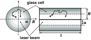
V.3 Tree dimensions
Consider the case when N ( r → ) 𝑁 → 𝑟 N(\vec{r}) r = R 𝑟 𝑅 r=R z = ± l 𝑧 plus-or-minus 𝑙 z=\pm l
Δ N ( r → ) − β 2 N ( r → ) = − f ( r → ) , N ( r → ) | r = R = 0 , N ( r → ) | z = ± l = 0 formulae-sequence Δ 𝑁 → 𝑟 superscript 𝛽 2 𝑁 → 𝑟 𝑓 → 𝑟 formulae-sequence evaluated-at 𝑁 → 𝑟 𝑟 𝑅 0 evaluated-at 𝑁 → 𝑟 𝑧 plus-or-minus 𝑙 0 \Delta N(\vec{r})-\beta^{2}N(\vec{r})=-f(\vec{r})\,,\quad N(\vec{r})\bigr{|}_{r=R}=0\,,\quad N(\vec{r})\bigr{|}_{z=\pm l}=0
The Green axially symmetric function satisfies the equation
Δ G ( r → , r → ′ ) − β 2 G ( r → , r → ′ ) = − δ ( r − r ′ ) δ ( z − z ′ ) 2 π r , G ( r → , r → ′ ) | r = R = 0 , G ( r → , r → ′ ) | z = ± l = 0 . formulae-sequence Δ 𝐺 → 𝑟 superscript → 𝑟 ′ superscript 𝛽 2 𝐺 → 𝑟 superscript → 𝑟 ′ 𝛿 𝑟 superscript 𝑟 ′ 𝛿 𝑧 superscript 𝑧 ′ 2 𝜋 𝑟 formulae-sequence evaluated-at 𝐺 → 𝑟 superscript → 𝑟 ′ 𝑟 𝑅 0 evaluated-at 𝐺 → 𝑟 superscript → 𝑟 ′ 𝑧 plus-or-minus 𝑙 0 \Delta G(\vec{r},\vec{r}^{\,\prime})-\beta^{2}G(\vec{r},\vec{r}^{\,\prime})=-\frac{\delta(r-r^{\prime})\delta(z-z^{\prime})}{2\pi r}\,,\quad G(\vec{r},\vec{r}^{\,\prime})\bigr{|}_{r=R}=0\,,\quad G(\vec{r},\vec{r}^{\,\prime})\bigr{|}_{z=\pm l}=0\,.
First consider the case R → ∞ → 𝑅 R\to\infty G ( r → , r → ′ ) 𝐺 → 𝑟 superscript → 𝑟 ′ G(\vec{r},\vec{r}^{\,\prime}) ϕ n ( z ) = sin π n 2 l ( l − z ) subscript italic-ϕ 𝑛 𝑧 𝜋 𝑛 2 𝑙 𝑙 𝑧 \phi_{n}(z)=\sin\frac{\pi n}{2l}\,(l-z) ϕ n ( ± l ) = 0 subscript italic-ϕ 𝑛 plus-or-minus 𝑙 0 \phi_{n}(\pm l)=0
G ( r → , r → ) = 1 2 π l ∑ n = 1 ∞ sin ( k n z ) sin ( k n z ′ ) I 0 ( λ n r < ) K 0 ( λ n r > ′ ) , where k n = π n 2 l , β n 2 = β 2 + k n 2 . formulae-sequence 𝐺 → 𝑟 → 𝑟 1 2 𝜋 𝑙 superscript subscript 𝑛 1 subscript 𝑘 𝑛 𝑧 subscript 𝑘 𝑛 superscript 𝑧 ′ subscript 𝐼 0 subscript 𝜆 𝑛 subscript 𝑟 subscript 𝐾 0 subscript 𝜆 𝑛 subscript superscript 𝑟 ′ where
formulae-sequence subscript 𝑘 𝑛 𝜋 𝑛 2 𝑙 subscript superscript 𝛽 2 𝑛 superscript 𝛽 2 superscript subscript 𝑘 𝑛 2 G(\vec{r},\vec{r})=\frac{1}{2\pi l}\sum\limits_{n=1}^{\infty}\sin(k_{n}z)\sin(k_{n}z^{\prime})I_{0}(\lambda_{n}r_{<})K_{0}(\lambda_{n}r^{\prime}_{>})\,,\quad\mbox{where}\quad k_{n}=\frac{\pi n}{2l}\,,\quad\beta^{2}_{n}=\beta^{2}+k_{n}^{2}\,. (35)
Finally, the axially symmetrical solution of the diffusion equation is
N ( r → ) = ∫ G ( r → , r → ) f ( r → ′ ) 𝑑 r → ′ = 2 π ∑ n = 1 ∞ sin k 2 n + 1 2 n + 1 ∫ 0 ∞ 𝑑 r ′ r ′ I 0 ( β 2 n + 1 r < ) K 0 ( β 2 n + 1 r > ) f ( r ′ ) . 𝑁 → 𝑟 𝐺 → 𝑟 → 𝑟 𝑓 superscript → 𝑟 ′ differential-d superscript → 𝑟 ′ 2 𝜋 superscript subscript 𝑛 1 subscript 𝑘 2 𝑛 1 2 𝑛 1 superscript subscript 0 differential-d superscript 𝑟 ′ superscript 𝑟 ′ subscript 𝐼 0 subscript 𝛽 2 𝑛 1 subscript 𝑟 subscript 𝐾 0 subscript 𝛽 2 𝑛 1 subscript 𝑟 𝑓 superscript 𝑟 ′ N(\vec{r})=\int G(\vec{r},\vec{r})f(\vec{r}^{\,\prime})\,d\vec{r}^{\,\prime}=\frac{2}{\pi}\sum\limits_{n=1}^{\infty}\frac{\sin k_{2n+1}}{2n+1}\int\limits_{0}^{\infty}dr^{\prime}\,r^{\prime}I_{0}(\beta_{2n+1}r_{<})K_{0}(\beta_{2n+1}r_{>})f(r^{\prime})\,.
Note that the integral over r 𝑟 r N ( r ) 𝑁 𝑟 N(r) β → β 2 n + 1 → 𝛽 subscript 𝛽 2 𝑛 1 \beta\to\beta_{2n+1} 28
The complex signal is
𝖲 ∞ ( 3 ) = 2 π ∬ 𝑑 r 𝑑 z r N ( r ) λ ( r ) = 4 l π 2 ∑ n = 0 ∞ 1 ( 2 n + 1 ) 2 ∫ 0 ∞ 𝑑 r r λ ( r ) N ( r ) , subscript superscript 𝖲 3 2 𝜋 double-integral differential-d 𝑟 differential-d 𝑧 𝑟 𝑁 𝑟 𝜆 𝑟 4 𝑙 superscript 𝜋 2 superscript subscript 𝑛 0 1 superscript 2 𝑛 1 2 superscript subscript 0 differential-d 𝑟 𝑟 𝜆 𝑟 𝑁 𝑟 \,\mathsf{S}^{(3)}_{\infty}=2\pi\iint dr\,dz\,rN(r)\lambda(r)=\frac{4l}{\pi^{2}}\sum\limits_{n=0}^{\infty}\frac{1}{(2n+1)^{2}}\int\limits_{0}^{\infty}dr\,r\lambda(r)N(r)\,,
or, denoting by 𝖲 ∞ ( 2 ) ( β ) subscript superscript 𝖲 2 𝛽 \,\mathsf{S}^{(2)}_{\infty}(\beta) 29
𝖲 ∞ ( 3 ) [ β n ] = 2 l π 2 ∑ n = 0 ∞ 𝖲 ∞ ( 2 ) [ β n ] ( 2 n + 1 ) 2 . subscript superscript 𝖲 3 delimited-[] subscript 𝛽 𝑛 2 𝑙 superscript 𝜋 2 superscript subscript 𝑛 0 subscript superscript 𝖲 2 delimited-[] subscript 𝛽 𝑛 superscript 2 𝑛 1 2 \,\mathsf{S}^{(3)}_{\infty}[\beta_{n}]=\frac{2l}{\pi^{2}}\sum\limits_{n=0}^{\infty}\frac{\,\mathsf{S}^{(2)}_{\infty}[\beta_{n}]}{(2n+1)^{2}}\,.
The same procedure can be used for R < ∞ 𝑅 R<\infty
G ( r → , r → ) = 1 2 π l ∑ n = 1 ∞ sin ( k n z ) sin ( k n z ′ ) [ I 0 ( β n R ) K 0 ( β n r > ) − I 0 ( β n r > ) K 0 ( β n R ) ] I 0 ( β n r < ) I 0 ( β n R ) , 𝐺 → 𝑟 → 𝑟 1 2 𝜋 𝑙 superscript subscript 𝑛 1 subscript 𝑘 𝑛 𝑧 subscript 𝑘 𝑛 superscript 𝑧 ′ delimited-[] subscript 𝐼 0 subscript 𝛽 𝑛 𝑅 subscript 𝐾 0 subscript 𝛽 𝑛 subscript 𝑟 subscript 𝐼 0 subscript 𝛽 𝑛 subscript 𝑟 subscript 𝐾 0 subscript 𝛽 𝑛 𝑅 subscript 𝐼 0 subscript 𝛽 𝑛 subscript 𝑟 subscript 𝐼 0 subscript 𝛽 𝑛 𝑅 G(\vec{r},\vec{r})=\frac{1}{2\pi l}\sum\limits_{n=1}^{\infty}\sin(k_{n}z)\sin(k_{n}z^{\prime})\bigl{[}I_{0}(\beta_{n}R)K_{0}(\beta_{n}r_{>})-I_{0}(\beta_{n}r_{>})K_{0}(\beta_{n}R)\bigr{]}\frac{I_{0}(\beta_{n}r_{<})}{I_{0}(\beta_{n}R)}\,, (36)
hence,
𝖲 R ( 3 ) = 2 π ∬ 𝑑 r 𝑑 z r N ( r ) λ ( r ) = 4 l π 2 ∑ n = 0 ∞ 1 ( 2 n + 1 ) 2 ∫ 0 R 𝑑 r r λ ( r ) N R ( r ) , subscript superscript 𝖲 3 𝑅 2 𝜋 double-integral differential-d 𝑟 differential-d 𝑧 𝑟 𝑁 𝑟 𝜆 𝑟 4 𝑙 superscript 𝜋 2 superscript subscript 𝑛 0 1 superscript 2 𝑛 1 2 superscript subscript 0 𝑅 differential-d 𝑟 𝑟 𝜆 𝑟 subscript 𝑁 𝑅 𝑟 \,\mathsf{S}^{(3)}_{R}=2\pi\iint dr\,dz\,rN(r)\lambda(r)=\frac{4l}{\pi^{2}}\sum\limits_{n=0}^{\infty}\frac{1}{(2n+1)^{2}}\int\limits_{0}^{R}dr\,r\lambda(r)N_{R}(r)\,,
again, denoting by 𝖲 R ( 2 ) ( β ) subscript superscript 𝖲 2 𝑅 𝛽 \,\mathsf{S}^{(2)}_{R}(\beta) 34
𝖲 R ( 3 ) [ β n ] = 2 l π 2 ∑ n = 0 ∞ 𝖲 R ( 2 ) [ β n ] ( 2 n + 1 ) 2 . subscript superscript 𝖲 3 𝑅 delimited-[] subscript 𝛽 𝑛 2 𝑙 superscript 𝜋 2 superscript subscript 𝑛 0 subscript superscript 𝖲 2 𝑅 delimited-[] subscript 𝛽 𝑛 superscript 2 𝑛 1 2 \,\mathsf{S}^{(3)}_{R}[\beta_{n}]=\frac{2l}{\pi^{2}}\sum\limits_{n=0}^{\infty}\frac{\,\mathsf{S}^{(2)}_{R}[\beta_{n}]}{(2n+1)^{2}}\,.
In this series only the first terms are significant for result (see fig. 2
Figure 2: Terms in power series 𝖲 R ( 3 ) subscript superscript 𝖲 3 𝑅 \,\mathsf{S}^{(3)}_{R} 𝖲 R ( 2 ) subscript superscript 𝖲 2 𝑅 \,\mathsf{S}^{(2)}_{R} 𝖲 R ( 3 ) subscript superscript 𝖲 3 𝑅 \,\mathsf{S}^{(3)}_{R}
Figure 3: The function S ( Δ ω ) 𝑆 Δ 𝜔 S(\Delta\omega) R = ∞ 𝑅 R=\infty R < ∞ 𝑅 R<\infty R 𝑅 R
Figure 4: The function S ( Δ ω ) 𝑆 Δ 𝜔 S(\Delta\omega) R = ∞ 𝑅 R=\infty R < ∞ 𝑅 R<\infty R 𝑅 R
Figure 5: The function S ( Δ ω ) 𝑆 Δ 𝜔 S(\Delta\omega) R < ∞ 𝑅 R<\infty R 𝑅 R l 𝑙 l
VI Discussion
The graphics of 𝖲 ( Δ ω ) 𝖲 Δ 𝜔 \,\mathsf{S}(\Delta\omega)
ν = 1000 , γ = 1 , v 0 = 100 , a = 1 . formulae-sequence 𝜈 1000 formulae-sequence 𝛾 1 formulae-sequence subscript 𝑣 0 100 𝑎 1 \nu=1000\,,\quad\gamma=1\,,\quad v_{0}=100\,,\quad a=1\,.
are presented at the figures.
Characteristic times are
τ a = 0.01 , τ γ = 1 , τ D = 0.1 . formulae-sequence subscript 𝜏 𝑎 0.01 formulae-sequence subscript 𝜏 𝛾 1 subscript 𝜏 𝐷 0.1 \tau_{a}=0{.}01\,,\quad\tau_{\gamma}=1\,,\quad\tau_{D}=0{.}1\,.
The values of R 𝑅 R R / a 𝑅 𝑎 R/a R = 2.0 , 3.0 , 5.0 𝑅 2.0 3.0 5.0
R=2{.}0\,,3{.}0\,,5{.}0
Acknowledgements.
We acknowledge support by CNES INTAS and NSAU (06-1000024-9075).