Searching for stochastic gravitational-wave background with the co-located LIGO interferometers

Abstract

This paper presents techniques developed by the LIGO Scientic Collaboration to search for the stochastic gravitational-wave background using the co-located pair of LIGO interferometers at Hanford, WA. We use correlations between interferometers and environment monitoring instruments, as well as time-shifts between two interferometers (described here for the first time) to identify correlated noise from non-gravitational sources. We veto particularly noisy frequency bands and assess the level of residual non-gravitational coupling that exists in the surviving data.

1 Introduction

The LIGO (Laser Interferometer Gravitational-Wave Observatory) project has constructed two detectors, dubbed H1 and H2, at its Hanford observatory (on the US Department of Energy’s Hanford Site in Washington, USA) and a third, L1, at its Livingston observatory (in Livingston Parish, Louisiana, USA). These detectors are Fabry-Perot, power-recycled Michelson interferometers that detect minute changes in the differential lengths of their arms, the signatures of incident gravitational waves. The Fabry-Perot cavities, or arms, are 4 km long in the H1 and L1 detectors and 2 km long in H2. In November 2005, the LIGO instruments achieved their design sensitivities [1] and began taking data for LIGO’s fifth science run, S5. The S5 observing effort continued through September 2007 and for some of its duration included the GEO 600 and VIRGO instruments. This run enables searches for different types of gravitational radiation with unprecedented sensitivities.

One of the LSC’s (LIGO Scientific Collaboration’s) major efforts is to search for an SGWB (stochastic gravitational-wave background), which is the gravitational analogue to the electromagnetic CMB (cosmic microwave background). The SGWB is predicted to contain contributions from unresolved populations of distant astrophysical processes involving compact objects as well as from early cosmological phenomena such as inflation and cosmic string collisions. The LSC has not yet finalized results for an SGWB search of the S5 data, but has published upper limits using S4 and earlier data sets [2][3][4].

1.1 The stochastic search and H1-H2

The SGWB is usually described in terms of the GW spectrum:

$$\Omega_{\mathrm{GW}}(f)\,\frac{\rmd f}{f}\equiv\frac{\rmd\rho_{\mathrm{GW}}}{\rho_{\mathrm{c}}},$$ (1)

where $\rmd\rho_{\rm GW}$ is the energy density of gravitational radiation contained in the frequency range $f$ to $f+\rmd f$ [5], $\rho_{\mathrm{c}}$ is the critical energy density of the Universe, and $f$ is frequency.

LSC searches for the isotropic component of the SGWB deploy the cross-correlation technique described in Allen and Romano[5]. The technique estimates the contribution to the detector noise due to the SGWB by cross-correlating the detector output between a pair of detectors; if the detectors’ intrinsic noises are uncorrelated, the common astrophysical component can be distinguished. We define the cross-correlation estimator:

$$Y=\int_{0}^{+\infty}\rmd f\;Y(f)=\int_{-\infty}^{+\infty}\rmd f\int_{-\infty}^{+\infty}\rmd f^{\prime}\;\delta_{T}(f-f^{\prime})\;\tilde{s}_{1}^{*}(f)\;\tilde{s}_{2}(f^{\prime})\;\tilde{Q}(f^{\prime})\,,$$ (2)

where $\delta_{T}$ is a finite-time approximation to the Dirac delta function, $\tilde{s}_{1}$ and $\tilde{s}_{2}$ are the Fourier transforms of the strain time-series of two interferometers, and $\tilde{Q}$ is a filter function. In the limit when the detector noise is much larger than the GW signal, and assuming that the detector noise is stationary, Gaussian, and uncorrelated between the two interferometers, the variance of the estimator $Y$ is given by:

$$\sigma_{Y}^{2}=\int_{0}^{+\infty}\rmd f\;\sigma_{Y}^{2}(f)\approx\frac{T}{2}\int_{0}^{+\infty}\rmd fP_{1}(f)P_{2}(f)|\tilde{Q}(f)|^{2}\,,$$ (3)

where the $P_{i}(f)$ are the one-sided power spectral densities (PSDs) of the two interferometers and $T$ is the (single-segment) integration time. Optimization of the signal-to-noise ratio leads to the following form of the optimal filter [5]:

$$\tilde{Q}(f)=\mathcal{N}\;\frac{\gamma(f)S_{\rm GW}(f)}{P_{1}(f)P_{2}(f)}{\rm\;,\;\;\;\;where\;\;\;}S_{\rm GW}(f)=\frac{3H_{0}^{2}}{10\pi^{2}}\;\frac{\Omega_{\rm GW}(f)}{f^{3}}\;.$$ (4)

Here, $S_{\rm GW}(f)$ is the strain power spectrum of the SGWB for which we are searching. Assuming a power-law template GW spectrum with index $\alpha$, $\Omega_{\rm GW}(f)=\Omega_{\alpha}(f/100{\rm\,Hz})^{\alpha}$, the normalization constant $\mathcal{N}$ is chosen such that $\langle Y\rangle=\Omega_{\alpha}T$. Finally, $\gamma(f)$ is the overlap reduction function. It captures the signal reduction due to two effects: (i) relative translation between interferometers introduces a frequency- and direction-dependent phase difference, and (ii) relative rotation makes each detector sensitive to a different polarization of incident radiation. As shown in figure 1, the identical antenna patterns of the collocated Hanford interferometers imply $\gamma(f)=1$, while for the H1-L1 pair, the overlap reduction is significantly lower than 1 above 50 Hz. In the most common search case, which assumes a frequency-independent spectrum ($\alpha=0$), the theoretical advantage for H1-H2 over H1-L1 is approximately a factor of ten in $\Omega_{0}$, as shown in figure 1. This advantage could be eroded, however, by instrumental correlations between H1 and H2.

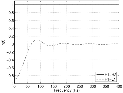
Figure 1: Left: Overlap reduction for the H1-H2 (black solid) and for the H1-L1 pairs (gray dashed). Right: Most recent upper limits (S3 (thin solid) and S4 (thick solid) runs) on $\Omega_{\alpha}$ as a function of $\alpha$, and sensitivity predictions for S5 for the H1-L1 (dashed) and H1-H2 (dot-dashed) pairs, assuming no instrumental correlations, design sensitivity, and one year of integration.

Since H1 and H2 share the same vacuum enclosures and many of their optical benches share the same building, they are susceptible to common environmental disturbances. The cross-correlation induced by the environment could be greater than the noise floor of our measurements, and could mimic, mask, or otherwise cause us to misestimate the amplitude or shape of a gravitational-wave signal. Hence, the H1-H2 pair has not been used for the SGWB searches so far.

We have developed two techniques to identify non-gravitational-wave correlations between H1 and H2 data. The IFO-PEM coherence technique was discussed in [6]. Here, IFO is shorthand for “interferometer” and PEM is an acronym for “physical environmental monitor”. There are numerous sensors situated throughout the LIGO observatories providing data to the PEM channels; there are accelerometers, magnetometers, seismometers, voltmeters, and anemometers. By computing the coherence spectrum between each IFO channel and each PEM channel, one can find the linear environmental coupling at each frequency. The technique is sensitive to features of arbitrary bandwidths and resolutions, but is restricted to linear couplings and obviously cannot give information where PEM coverage is non-existent.

Section 2 of this paper will describe the second, complementary handle on non-gravitational coupling, the time-shift technique. The time-shift technique’s added value is that it is not hindered by incomplete knowledge of the environment; its trade-off is in its narrow bandwidth. Section 3 will connect the two methods to each other and to the measured quantities in the SGWB search and section 4 will describe how we envision applying these techniques together to extract the best possible SGWB measurement from the H1-H2 pair. The paper will close with a statement of where we stand on the H1-H2 problem.

2 Time-shift technique

The main idea of the time-shift technique is to perform the search described in the previous section after introducing an unphysical time-shift between the two interferometers’ data-streams. That is, since the SGWB is expected to be broadband (at least hundreds of Hz wide), the SGWB-induced cross-correlation between the two interferometers is expected to disappear after a time-shift $\tau$ larger than $\sim 10$ ms and only narrowband features, of order $1/\tau$ wide or narrower, are expected to be present in the time-shifted estimates of $Y(f)$. Note that such narrowband features could be instrumental/environmental in nature, but they could also be genuine GW signals. Since narrowband GW signals are not a target of this search, our approach is to remove all narrow-band features from our analysis, regardless of their origin. Further note that a narrowband feature could also be a statistical fluctuation. In this case, it would not appear in the analysis with different time-shifts, and it would then have to be included in the search for the SGWB. While the time-shift technique is not susceptible to the “incomplete coverage” issues that are relevant for the IFO-PEM coherence technique, it cannot identify broadband instrumental correlations. Hence, the two techniques are largely complementary.

In order to avoid correlations between estimates with different time-shifts $\tau$, the analysis must be performed using segment duration $T\leq\tau$. Since we are interested in removing $\sim 1$ Hz features and narrower, we use time-shifts of order 1 s. This also leads to the choice $T=1$ s. Such short segment duration leads to other differences from the standard SGWB search procedure (where $T\sim 100$ s), described in the references [2][3][4]. In particular, the PSD estimates are obtained using seven neighboring 1 s segments on each side (instead of only one), and the data quality cuts are imposed on the PSDs rather than on estimates of $\sigma_{Y}$, as they are less susceptible to downward fluctuations in the noise. We also remove the times identified by the LSC Glitch Group to contain instrumentally caused transients in the data. The method was tested using the S5 data between November 2005 and April 2006, using the calibrated strain data, a 40-500 Hz frequency range, a sixth-order butterworth high-pass filter at 32 Hz to remove low-frequency detector noise, and 50% overlapping Hann windows. In the study, we never estimated $Y(f)$ without an unphysical time-shift, to avoid potentially biasing the resulting data-quality cuts.

We define the frequency-dependent signal-to-noise ratio, as a function of time-shift $\tau$, properly accounting for the frequency bin width $\rmd f$:

$${\rm SNR_{TS}}(f;\tau)=\frac{|Y(f;\tau)|\;\rmd f}{\sigma(f;\tau)\;\sqrt{{\rm d}f}}.$$ (5)

Using 1 s segments, we performed $\pm 1,\pm 2$ s time-shifts. We then attempted three ways of combining these four measurements to estimate the the SNR at zero-shift, ${\rm SNR_{TS}}(f;0)$: Gaussian fit to the four measurements, maximum over the four measurements, and average of $\pm 1$ s measurements. These three approaches led to very similar results, so in the following we conservatively use the maximum over the three.

3 Comparison of the two techniques

The PEM-IFO coherence method estimates the environmental contribution to the coherence between the two interferometers $\gamma_{\mathrm{PEM}}(f)$. Coherence $\gamma(f)$ is defined by:

$$\gamma(f)=\frac{P_{12}(f)}{\sqrt{P_{1}(f)P_{2}(f)}}=\frac{P_{12}(f)Q(f)\rmd f}{\sqrt{P_{1}(f)P_{2}(f)Q^{2}(f)\rmd f/\mathcal{T}}}\;\frac{1}{\sqrt{\mathcal{T}\rmd f}}=\frac{{\rm SNR}(f)}{\sqrt{\mathcal{T}\rmd f}},$$ (6)

where $P_{12}(f)=\langle s_{1}^{*}(f)s_{2}(f)\rangle$ is the cross-power spectral density and $\mathcal{T}$ is the total observation time, so $\mathcal{T}\rmd f$ is the total number of segments. Hence, we can estimate the environmental contribution to the SNR of the stochastic search:

$${\rm SNR_{PEM}}(f)=\gamma_{{\rm PEM}}(f)\sqrt{\mathcal{T}\rmd f}.$$ (7)

This allows us to directly compare the two techniques, keeping in mind that ${\rm SNR_{TS}}$ is defined using $|Y(f)|$. Moreover, we can define the environmental contribution to the point estimate, where again, the PEM subscript indicates that the quantity is estimated using the PEM-IFO coherence method:

$$\Omega_{\rm PEM}(f)=\frac{Y_{\rm PEM}(f)}{T}=\frac{\gamma_{\rm PEM}(f)\sigma(f)}{\sqrt{T}}.$$ (8)

4 Proposed search algorithm

4.1 Veto

The first obvious application of the described techniques is to veto frequencies in which H1 and H2 exhibit strong non-gravitational coupling. Figure 2 compares the SNR estimates using the two techniques. Note that the two techniques generally agree well in identifying contaminated frequency bands. These bands will be vetoed in the SGWB search. It is not completely self-evident precisely how this veto should be defined, since the IFO channels are coupled to some extent at all frequencies. One approach is to veto frequency bins in which both methods’ SNRs exceed 2. This choice is somewhat relaxed, and it relies on the assumption that we can estimate $\Omega_{\rm PEM}$ in the remaining frequency bands that pass the veto, as discussed below.

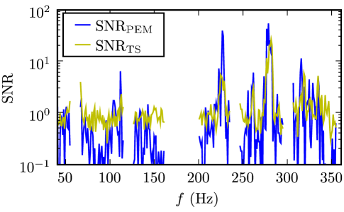
Figure 2: Comparison of the PEM-IFO coherence and time-shift techniques for estimating the contaminated frequency bands. The 60 Hz harmonics have already been vetoed.

4.2 Estimate the residual environmental contribution

Using equation 8, we can estimate the environmental contribution to the estimate of the SGWB amplitude $\Omega_{\rm PEM}$, in the frequency bands that pass the veto described in section 4.1. This estimate could be potentially subtracted from the overall SGWB amplitude estimate, thereby producing a better estimate of the gravitational-wave contribution.

In this case, it is important to understand the uncertainty in the estimate of $\Omega_{\rm PEM}$. The statistical uncertainty in $\Omega_{\rm PEM}$ comes from the statistical uncertainties on $\gamma_{\rm PEM}$ and on $\sigma_{Y}$, both of which are expected to be negligible compared to the theoretical uncertainty on the overall amplitude estimate $\sigma_{\Omega}=\sigma_{Y}/T$.

4.3 Estimate systematics

The systematic error on $\Omega_{\rm PEM}$ could potentially be large. A few major sources of uncertainty are apparent: the approximation made in the definition of $\gamma_{\rm PEM}$ from the individual IFO-PEM coherences [6] and differences in the details of the data manipulation between the IFO-PEM coherence and SGWB search calculations. One approach for estimating this systematic error is to compare the $\Omega_{\rm PEM}$ estimate with the SGWB estimate in a frequency band that is known to be dominated by environmental correlations. As the environment dominates, $\Omega_{\rm PEM}$ should explain the entire SGWB estimate of $\Omega_{0}$ in this band. The mismatch would give us an estimate on the systematic error of our IFO-PEM coherence measurement.

We have performed such a calculation. Our preliminary results indicate that the IFO-PEM and the SGWB estimates agree within 50% in the contaminated frequency bands. However, we believe we can significantly improve this agreement; the differences in the data manipulation in the two techniques (segment duration, frequency resolution, PSD weighting, etc) were significant and we expect to minimize them in future iterations.

Another indication of the systematic error could be obtained from hardware injections. At semi-regular intervals in the LIGO science runs, we injected simulated SGWB signals by physically shaking the optics; the SGWB search on these segments tests how accurately we can recover the injected signal’s amplitude. If we instead treat the injection data stream as a PEM channel, we can verify that we can subtract out the injection and instead produce an estimate consistent with noise. A signal detection would imply an imperfect subtraction.

4.4 SGWB search

Having identified the most egregiously correlated frequency bands, and estimated the environmental contribution $\Omega_{\rm PEM}$, we can proceed with the usual SGWB search algorithm. This includes a number of diagnostics on the quality of data, such as tests of Gaussianity, long-term stationarity, etc. Potential problems would become apparent here, such as omissions in the frequency and time vetoes. Any problems would be investigated and used as input in another iteration of the veto and environment contribution estimation steps. The very last step is to produce the SGWB estimate, and potentially subtract the $\Omega_{\rm PEM}$ estimate.

5 Conclusions

We have presented the time-slide technique, by which all narrowband, correlated noise between two interferometers can be identified. It provides complementary coverage of the space of possible non-gravitational couplings between the interferometers, alongside the IFO-PEM coherence technique. It is important to note that these techniques leave some blind spots: they leave out the possibility of broad-band environmental contributions that are unmonitored in the observatory’s environment, and they misestimate their contributions if the couplings are non-linear. This includes effects such as seismic upconversion, a non-linear process by which low-frequency seismic activity excites higher-frequency vibrations in the instrument, and stray light reflections in the beam tubes that introduce cross-talk between the interferometers.

We would like to acknowledge many useful discussions with members of the LIGO Scientific Collaboration stochastic analysis group which were critical in the formulation of the methods and results described in this paper. This work has been supported in part by NSF grants PHY-0200852 and PHY-0701817. LIGO was constructed by the California Institute of Technology and Massachusetts Institute of Technology with funding from the National Science Foundation and operates under cooperative agreement PHY-0107417. This paper has the LIGO Document Number LIGO-P070128-00-Z.

References

References

- [1] LIGO laboratory home page for interferometer sensitivities. URL: http://www.ligo.caltech.edu/jzweizig/distribution/LSC_Data/.
- [2] Abbott et al. Searching for a stochastic background of gravitational waves with LIGO. ApJ, 659:918–930, 2007. arXiv:astro-ph/0608606.
- [3] Abbott et al. Upper limits on a stochastic background of gravitational waves. Phys. Rev. Lett., 95(221101), 2005. arXiv:astro-ph/0507254.
- [4] Abbott et al. Analysis of first LIGO science data for stochastic gravitational waves. Phys. Rev. D, 69(122004), 2004. arXiv:gr-qc/0312088.
- [5] Allen B and Romano J. Detecting a stochastic background of gravitational radiation: Signal processing strategies and sensitivities. Phys. Rev. D, 59(102001), October 1997. arXiv:gr-qc/9710117.
- [6] Fotopoulos N for the LIGO Scientific Collaboration. Identifying correlated environmental noise in co-located interferometers with application to stochastic gravitational wave analysis. Class. Quantum Grav, 23:S693–S704, 2006.