Invariant manifolds as building blocks for the formation of spiral arms and rings in barred galaxies

We propose a theory to explain the formation of spiral arms and of all types of outer rings in barred galaxies, extending and applying the technique used in celestial mechanics to compute transfer orbits. Thus, our theory is based on the chaotic orbital motion driven by the invariant manifolds associated to the periodic orbits around the hyperbolic equilibrium points. In particular, spiral arms and outer rings are related to the presence of heteroclinic or homoclinic orbits. Thus, $R_{1}$ rings are associated to the presence of heteroclinic orbits, while $R_{1}R_{2}$ rings are associated to the presence of homoclinic orbits. Spiral arms and $R_{2}$ rings, however, appear when there exist neither heteroclinic nor homoclinic orbits. We examine the parameter space of three realistic, yet simple, barred galaxy models and discuss the formation of the different morphologies according to the properties of the galaxy model. The different morphologies arise from differences in the dynamical parameters of the galaxy.

1 Introduction

Bars are a very common feature of disc galaxies. In a sample of $186$ spirals, $56\%$ of the galaxies in the near infrared are strongly barred, while an additional $16\%$ are weakly barred esk00 . A large fraction of barred galaxies show two clearly defined spiral arms elm82 , departing from the end of the bar. This is the case for instance in NGC 1300, NGC 1365 and NGC 7552. Spiral arms are believed to be density waves in a disc galaxy lind63 . In too69 , Toomre found that the spiral waves propagate towards the principal Lindblad resonances of the galaxy, where they damp down, and thus concludes that long-lived spirals need some replenishment. Danby argued that orbits in the gravitational potential of a bar play an important role in the formation of arms dan65 and Kaufmann & Contopoulos argue that, in self-consistent models for three real barred spiral galaxies, spiral arms are supported also by chaotic orbits kau96 .

The origin of rings has been studied by Schwarz who calculated the response of a gaseous disc galaxy to a bar perturbation sch81 ; sch84 ; sch85 . He proposed that ring-like patterns are associated to the principal orbital resonances, namely ILR (Inner Lindblad Resonance), CR (Corotation Resonance), and OLR (Outer Lindblad Resonance). There are different types of outer rings. Buta classified them according to the relative orientation of the ring and bar major axes but95 . If these two are perpendicular, the outer ring is classified as $R_{1}$. If they are parallel, the outer ring is classified as $R_{2}$. Finally, if both types of rings are present in the galaxy, the outer ring is classified as $R_{1}R_{2}$.

In Romero-Gómez et al. rom06 ; rom07 , we note that spiral arms and rings emanate from the ends of the bar and we propose that rings and spiral arms are the result of the orbital motion driven by the invariant manifolds associated to the Lyapunov periodic orbits around the unstable equilibrium points. In Romero-Gómez et al. rom06 , we fix a barred galaxy potential and we study the dynamics around the unstable equilibrium points. We give a detailed definition of the invariant manifolds associated to a Lyapunov periodic orbit. For the model considered, the invariant manifolds delineate well the loci of an $rR_{1}$ ring structure, i.e. a structure with an inner ring (r) and an outer ring of the type $R_{1}$. In Romero-Gómez et al. rom07 , we construct families of models based on simple, yet realistic, barred galaxy potentials. In each family, we vary one of the free parameters of the potential and keep the remaining fixed. For each model, we numerically compute the orbital structure associated to the invariant manifolds. In this way, we are able to study the influence of each model parameter on the global morphologies delineated by the invariant manifolds.

Voglis, Stavropoulos & Kalapotharakos study the chaotic motion present in self-consistent models of both rotating and non-rotating galaxies, concluding that rotating models are characterised by larger fractions of mass in chaotic motion vog06a . Patsis argues that the spiral arms of NGC 4314 are due to chaotic orbits and, to show it, he computes families of orbits with initial conditions near the unstable equilibrium points pat06 . Voglis, Tsoutsis & Efthymiopoulos vog06b reproduce a spiral pattern found in a self-consistent simulation using the apocentric invariant manifolds of the short-period family of unstable periodic orbits. They give the angular position of the apocentres, which is where they state the stars spend a large part of their radial period, as a soliton-type solution of the Sine-Gordon equation.

In Sect. 2, we first present the galactic models used in the computations and the equations of motion. In Sect. 3, we give a brief description of the dynamics around the unstable equilibrium points and the role the invariant manifolds play in the transfer of matter around the galaxy. In Sect. 4, we show the different morphologies that result from the computations.

2 Description of the model and equations of motion

In this section, we first describe the bar models used in the computations by giving the density distributions, or the potentials used. We then write the equation of motion and we define the effective potential and Jacobi constant.

2.1 Description of the model

We use three different models, all three consisting of the superposition of an axisymmetric component and another bar-like. Our first model is that of Athanassoula ath92 . The axisymmetric component is composed of a disc, modelled as a Kuzmin-Toomre disc kuz56 ; too63 of surface density $\sigma(r)$:

$$\sigma(r)=\frac{V_{d}^{2}}{2\pi r_{d}}\left(1+\frac{r^{2}}{r_{d}^{2}}\right)^{-3/2},$$ (1)

and a spheroid modelled by a density distribution of the form $\rho(r)$:

$$\qquad\rho(r)=\rho_{b}\left(1+\frac{r^{2}}{r_{b}^{2}}\right)^{-3/2}.$$ (2)

The parameters $V_{d}$ and $r_{d}$ set the scales of the disc velocities and radii, respectively, and $\rho_{b}$ and $r_{b}$ determine the concentration and scale-length of the spheroid.

Our bar potential is described by a Ferrers ellipsoid fer77 whose density distribution is:

$$\left\{\begin{array}[]{lr}\rho_{0}(1-m^{2})^{n}&m\leq 1\\ 0&m\geq 1,\end{array}\right.$$ (3)

where $m^{2}=x^{2}/a^{2}+y^{2}/b^{2}$. The values of $a$ and $b$ determine the shape of the bar, $a$ being the length of the semi-major axis, which is placed along the $x$ coordinate axis, and $b$ being the length of the semi-minor axis. The parameter $n$ measures the degree of concentration of the bar and $\rho_{0}$ represents the bar central density.

We also use two further ad-hoc bar potentials, namely a Dehnen’s bar type, $\Phi_{1}$, (Dehnen deh00 ):

$$\Phi_{1}(r,\theta)=-\frac{1}{2}\epsilon v_{0}^{2}\cos(2\theta)\left\{{\begin{array}[]{ll}\displaystyle 2-\left(\frac{r}{\alpha}\right)^{n},&r\leq\alpha\rule[-14.22636pt]{0.0pt}{28.45274pt}\\ \displaystyle\left(\frac{\alpha}{r}\right)^{n},&r\geq\alpha.\rule[-14.22636pt]{0.0pt}{28.45274pt}\end{array}}\right.,$$ (4)

and a Barbanis-Woltjer (BW) bar type, $\Phi_{2}$, (Barbanis & Woltjer bar67 ):

$$\Phi_{2}(r,\theta)=\hat{\epsilon}\sqrt{r}(r_{1}-r)\cos(2\theta)$$ (5)

The parameter $\alpha$ is a characteristic length scale of the Dehnen’s type bar potential, and $v_{0}$ is a characteristic circular velocity. The parameter $\epsilon$ is related to the bar strength. The parameter $r_{1}$ is a characteristic scale length of the BW bar potential and the parameter $\hat{\epsilon}$ is related to the bar strength.

2.2 Equations of motion

In order to compute the equations of motion, we take into account that the bar component rotates anti-clockwise with angular velocity ${\bf\Omega_{p}}=\Omega_{p}{\bf z}$, where $\Omega_{p}$ is a constant pattern speed  . The equations of motion in this potential in a frame rotating with angular speed ${\bf\Omega_{p}}$ in vector form are

$${\bf\ddot{r}=-\nabla\Phi}-2{\bf(\Omega_{p}\times\dot{r})-\Omega_{p}\times(\Omega_{p}\times r)},$$ (6)

where the terms $-2{\bf\Omega_{p}\times\dot{r}}$ and $-{\bf\Omega_{p}\times(\Omega_{p}\times r)}$ represent the Coriolis and the centrifugal forces, respectively, and ${\bf r}$ is the position vector. Defining an effective potential:

$$\Phi_{\hbox{\scriptsize eff}}=\Phi-\frac{1}{2}\Omega_{p}^{2}\,(x^{2}+y^{2}),$$ (7)

Eq. (6) becomes ${\bf\ddot{r}=-\nabla\Phi_{\hbox{\scriptsize eff}}}-2{\bf(\Omega_{p}\times\dot{r})},$ and the Jacobi constant is $E_{J}=\frac{1}{2}{\bf\mid\dot{r}\mid}^{2}+\Phi_{\hbox{\scriptsize eff}},$ which, being constant in time, can be considered as the energy in the rotating frame.

3 Dynamics around $L_{1}$ and $L_{2}$

For our calculations we place ourselves in a frame of reference corotating with the bar and place the bar major axis along the $x$ axis. In this rotating frame we have five equilibrium points, which, due to the similarity with the Restricted Three Body Problem, are called Lagrangian points. The points located on the origin of coordinates, namely $L_{3}$, and along the $y$ axis, namely $L_{4}$ and $L_{5}$, are linearly stable. The ones located symmetrically along the $x$ axis, namely $L_{1}$ and $L_{2}$, are linearly unstable. Around the equilibrium points there exist families of periodic orbits, e.g. around the central equilibrium point the well-known $x_{1}$ family of periodic orbits con80 that is responsible for the bar structure.

The dynamics around the unstable equilibrium points is described in detail in rom06 ; here we give only a brief summary. Around each unstable equilibrium point there also exists a family of periodic orbits, known as the family of Lyapunov orbits lya49 . For a given energy level, two stable and two unstable sets of asymptotic orbits emanate from the periodic orbit, known as the stable and the unstable invariant manifolds, respectively. We denote by $W_{\gamma_{i}}^{s}$ the stable invariant manifold associated to the periodic orbit $\gamma$ around the Lagrangian point $L_{i},\,i=1,2$. The stable invariant manifold is the set of orbits that tends to the periodic orbit asymptotically. Similarly, we denote by $W_{\gamma_{i}}^{u}$ the unstable invariant manifold associated to the periodic orbit $\gamma$ around the Lagrangian point $L_{i},\,i=1,2$. The unstable invariant manifold is the set of orbits that departs asymptotically from the periodic orbit (i.e. orbits that tend to the Lyapunov orbits when the time tends to minus infinity) (Fig. 1). Since the invariant manifolds extend well beyond the neighbourhood of the equilibrium points, they can be responsible for global structures.

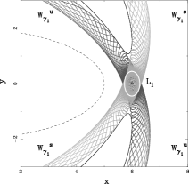
Figure 1: Unstable (in dark grey), $W_{\gamma_{1}}^{u}$, and stable (in light grey), $W_{\gamma_{1}}^{s}$, invariant manifolds associated to the periodic orbit around $L_{1}$ (in white solid line). In black solid lines, we plot the zero velocity curves for this energy level and the dashed curve shows the outline of the bar.

In rom07 , we give a detailed description of the role invariant manifolds play in global structures and, in particular, in the transfer of matter. Simply speaking, the transfer of matter is characterised by the presence of homoclinic, heteroclinic, and transit orbits. Homoclinic orbits correspond to asymptotic trajectories $\psi$ such that $\psi\in W_{\gamma_{i}}^{u}\cap W_{\gamma_{i}}^{s},\,i=1,2$. That is, they are asymptotic orbits that depart from the unstable Lyapunov periodic orbit $\gamma$ around $L_{i}$ and return asymptotically to it (Fig. 2a). Heteroclinic orbits are asymptotic trajectories $\psi^{\prime}$ such that $\psi^{\prime}\in W_{\gamma_{i}}^{u}\cap W_{\gamma_{j}}^{s},\,i,j=1,2,\,i\neq j$. That is, they are asymptotic orbits that depart from the periodic orbit $\gamma$ around $L_{i}$ and asymptotically approach the corresponding Lyapunov periodic orbit with the same energy around the Lagrangian point at the opposite end of the bar $L_{j}$, $i\neq j$ (Fig. 2b). We are interested in the homoclinic and heteroclinic orbits corresponding to the first intersection of the invariant manifolds with an appropriate surface of section. There exist also trajectories that spiral out from the region of the unstable periodic orbit and we refer to them as transit orbits (Fig. 2c). These three types of orbits are chaotic orbits since they fill part of the chaotic sea when we plot the Poincaré surface of section (e.g. the section $(x,\dot{x})$ near $L_{1}$).

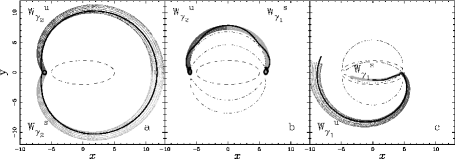
Figure 2: Homoclinic (a), heteroclinic (b) and transit (c) orbits (black thick lines) in the configuration space. In dark grey lines, we plot the unstable invariant manifolds associated to the periodic orbits, while in light grey we plot the corresponding stable invariant manifolds. In dashed lines, we give the outline of the bar and, in (b) and (c), we plot the zero velocity curves in dot-dashed lines.

4 Results

One of our goals is to check the influence of each main free parameter of the models introduced in Sect. 2. In order to do so, we make families of models in which only one of the free parameters is varied, while the others are kept fixed. Our results in rom07 show that only the bar pattern speed and the bar strength have a considerable influence on the shape of the invariant manifolds and, thus, on the morphology of the galaxy. Having established this, we perform a two-dimensional parameter study for each bar potential and we obtain all types of rings and spiral arms.

In Fig. 3 we show the model rings and the spiral structure we obtain with our models. We plot the unstable (Fig. 3a, b and d) and the unstable and stable (Fig. 3c) invariant manifolds associated to one of the Lyapunov periodic orbits of the main family around $L_{1}$ and $L_{2}$. Note that we plot the projection of the invariant manifolds on the configuration space $(x,y)$. Our results show that the morphologies obtained depend on dynamical factors, that is, on the presence of homoclinic or heteroclinic orbits of the first intersection of the corresponding invariant manifolds. If heteroclinic orbits exist, then the ring of the galaxy is classified as $rR_{1}$ (Fig. 3a). The inner branches of the invariant manifolds associated to $\gamma_{1}$ and $\gamma_{2}$ outline a nearly elliptical inner ring that encircles the bar. The outer branches of the same invariant manifolds form an outer ring whose principal axis is perpendicular to the bar major axis. If the model has neither heteroclinic, nor homoclinic orbits and only transit orbits are present, the barred galaxy will present two spiral arms emanating from the ends of the bar. The outer branches of the unstable invariant manifolds will spiral out from the ends of the bar and they extend azimuthally to more than $3\pi/2$ (Fig. 3d). If the outer branches of the unstable invariant manifolds intersect in configuration space with each other , then they form the characteristic shape of $R_{2}$ rings (Fig. 3b). That is, the trajectories outline an outer ring whose major axis is parallel to the bar major axis. The last possibility is if only homoclinic orbits exist. In this case, the inner branches of the invariant manifolds form an inner ring, while the outer branches outline both types of outer rings, thus the barred galaxy presents an $R_{1}R_{2}$ ring morphology (Fig. 3c).

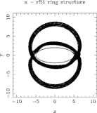
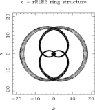
Figure 3: Model rings and spiral arm structures. We plot characteristic examples of (a) $rR_{1}$ ring structure, (b) $rR_{2}$ ring structure, (c) $R_{1}R_{2}$ ring structure and (d) Spiral arms.

We also study the response of an axisymmetric component to a bar perturbation. We use the same axisymmetric potential and the same bar potential as in our models and the bar is introduced gradually, to avoid transients. Once the bar has reached its maximum amplitude, we consider a snapshot of the response simulation and we compare its morphology to the corresponding structure we obtain with our models. In Fig. 4 we show the results for the spiral arms case, by over-plotting the selected snapshot with our model. The white points represent the particle positions of the response study and the black lines are the unstable invariant manifolds. Note that the two match perfectly.

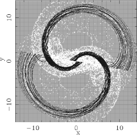
Figure 4: Over-plot of the results obtained with the response simulation (white dots) and the invariant manifolds (black lines) in a model with spiral arms.

We compare our results with observational data (E. Athanassoula, M. Romero-Gómez, J.J. Masdemont, C. García-Gómez, in preparation) and we find good agreement. Regarding the photometry, the density profiles across radial cuts in rings and spiral arms agree with the ones obtained from observations. The velocities along the ring also show that these are only a small perturbation of the circular velocity.

References

- (1) E. Athanassoula: Phys. Rep. 114, 319 (1984)
- (2) E. Athanassoula: MNRAS 259, 328 (1992)
- (3) B. Barbanis, L. Woltjer: ApJ 150, 461 (1967)
- (4) R. Buta: ApJS 96, 39 (1995)
- (5) G. Contopoulos, Th. Papayannopoulos: A& A, 92, 33 (1980)
- (6) J.M.A. Danby: AJ 70, 501 (1965)
- (7) W. Dehnen: AJ 119, 800 (2000)
- (8) D.M. Elmegreen, B.G. Elmegreen: MNRAS 201, 1021 (1982)
- (9) P.B. Eskridge, J.A. Frogel, R.W. Podge, et al.: AJ 119, 536 (2000)
- (10) N.M. Ferrers: Q.J. Pure Appl. Math. 14, 1 (1877)
- (11) D.E. Kaufmann, G. Contopoulos: A& A, 309, 381 (1996)
- (12) G. Kuzmin: Astron. Zh. 33, 27 (1956)
- (13) B. Lindblad: Stockholms Observatorium Ann. Vol. 22, No. 5 (1963)
- (14) A. Lyapunov: Ann. Math. Studies 17 (1949)
- (15) P.A. Patsis: MNRAS 369, L56 (2006)
- (16) M. Romero-Gómez, J.J. Masdemont, E. Athanassoula, C. García-Gómez: A & A 453, 39 (2006)
- (17) M. Romero-Gómez, E. Athanassoula, J.J. Masdemont, C. García-Gómez: A & A 472, 63 (2007)
- (18) M.P. Schwarz: ApJ 247, 77 (1981)
- (19) M.P. Schwarz: MNRAS 209, 93 (1984)
- (20) M.P. Schwarz: MNRAS 212, 677 (1985)
- (21) A. Toomre: ApJS 138, 385 (1963)
- (22) A. Toomre: ApJ 158, 899 (1969)
- (23) N. Voglis, I. Stavropoulos, C. Kalapotharakos: MNRAS 372, 901 (2006)
- (24) N. Voglis, P. Tsoutsis, C. Efthymiopoulos: MNRAS 373, 280 (2006)