W-like states of $N$ uncoupled spins $\frac{1}{2}$

Abstract

The exact dynamics of a disordered spin star system, describing a central spin coupled to $N$ distinguishable and non interacting spins $\frac{1}{2}$, is reported. Exploiting their interaction with the central single spin system, we present possible conditional schemes for the generation of W-like states, as well as of well-defined angular momentum states, of the $N$ uncoupled spins. We provide in addition a way to estimate the coupling intensity between each of the $N$ spins and the central one. Finally the feasibility of our procedure is briefly discussed.

1 Introduction

Interacting spin models play a central role in many physical contexts providing a paradigm to describe a wide range of different systems. In condensed matter physics, for example, they can be explored to analyze many properties of magnetic compounds. It is indeed well known that a suitable general model of a magnet consists of $N$ spins coupled by exchange interaction with arbitrary range and strength.

The interest toward spin systems, and more in particular toward spin dynamics in semiconductor structures, has remarkably increased in the last few years also in connection with the new emerging areas of quantum computation and information Bayat -Plenio . In these contexts, spin models like Heisenberg spin chains or spin star systems, describing for example a single electron spin in a semiconductor quantum dot interacting with surrounding nuclear spins via hyperfine coupling mechanisms, have been extensively studied Pratt -Breuer .

Generally speaking spin models have proved to be promising candidates for the generation and the control of assigned quantum correlations, as witnessed by the numerous papers recently appeared in literatureVerstraete -Binosi .

In this paper we concentrate on the possibility of manipulating at demand the state of a sample of $N$ uncoupled spins exploiting their common interaction with another single spin called central system. The analysis we have developed, on the one hand provides possible procedures to guide the system toward pure states characterized by fixed correlation conditions, on the other hand suggests a way to to estimate the coupling strenght between each of the $N$ spins and the central one.

2 Disordered spin star system

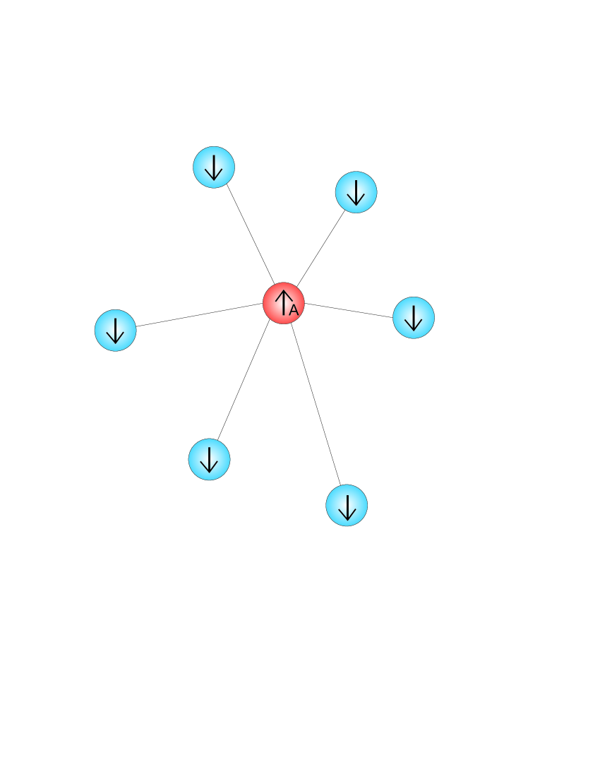
Figure 1: An illustration of a disordered spin star system

Having in mind as objective the possibility of generating fixed entanglement conditions in a system of $N$ uncoupled spins $\frac{1}{2}$, we exploit the interaction of each element of the system with another spin $\frac{1}{2}$ hereafter called central one. The system we are talking about is illustrated for convenience in Figure 1 and it can be described adopting the following hamiltonian model:

$$H=H_{0}+H_{I}$$ (1)

with

$$H_{0}=\omega\sum_{j=1}^{N}\sigma_{z}^{j}+\omega_{0}\sigma_{z}^{A},$$ (2)

$$H_{I}=\sum_{j=1}^{N}\alpha_{j}(\sigma_{+}^{A}\sigma_{-}^{j}+\sigma_{-}^{A}\sigma_{+}^{j}),$$ (3)

The Pauli operators labelled by the index $A$ refer to the central spin, while the others characterized by the index $j$ ($j=1..N$) refer to the $N$ spins. The coupling strength between the spin $j$ and the central one is measured by the constant $\alpha_{j}$ and, generally speaking, $\alpha_{j}$ may be different from $\alpha_{i}$ for $j\neq i$. In realistic physical situations the coupling constants can change for example proportionally to the distance from the central system Braktavatsala . We refer to the system described by eq. (1) as disordered spin star system.

Studying the dynamical properties of this model is for example of interest in contexts like quantum dot coupled by hyperfine interaction with nuclear spins, or electronic spins bound to phosphorus atoms in a matrix of silica or germanio in presence of defects Schliemann .

The symmetry properties of the hamiltonian model can be successfully exploited in order to analyze the dynamics of the system. It is easy to convince oneself that the component along the $z$ axes of the total angular momentum operator $S_{z}=\frac{\sigma_{z}^{A}}{2}+\frac{1}{2}\sum_{j=1}^{N}\sigma_{z}^{j}=\frac{\sigma_{z}^{A}}{2}+J_{z}$ is a constant of motion. Then, starting from an eigenstate of $S_{z}$ the system evolves in the correspondent invariant Hilbert subspace. Let’s suppose in particular to prepare the system in the following state

$$|\psi_{\{i_{1},...i_{p}\}}(0)\rangle=|\!\!\uparrow_{A}\rangle|\!\!\downarrow\ldots\uparrow_{i_{1}}\ldots\uparrow_{i_{p}}\ldots\downarrow\rangle,$$ (4)

where the central spin, as well as $p$ of the $N$ spins, namely the $i_{1}$-th, $i_{2}$-th,… $i_{p}$th, are in their respective up state $|\!\!\uparrow\rangle$ defined as $\sigma_{z}^{i}|\!\!\uparrow\rangle=|\!\!\uparrow\rangle$ with $i=A,1,..,N$, whereas the others are in their down state $|\!\!\downarrow\rangle$ with $\sigma_{z}^{i}|\!\!\downarrow\rangle=-|\!\!\downarrow\rangle$.

We in addition denote the state $|\!\!\uparrow_{A}\rangle|\!\!\downarrow,\downarrow,\ldots,\downarrow\rangle$, where all the uncoupled spins are down, by $|\psi_{0}(0)\rangle$.

Taking into account the previous considerations we may claim that, at time instant $t$ the state of the system prepared in the state (4) can be written as

$$|\psi_{\{i_{1},...i_{p}\}}(t)\rangle= \sum_{j_{1}<j_{2}<\ldots<j_{p}}a_{j_{1},j_{2},\ldots,j_{p}}(t)|\!\!\uparrow_{A}\rangle|\!\!\downarrow\ldots\uparrow_{j_{1}}\ldots\uparrow_{j_{p}}\ldots\downarrow\rangle+$$ (5)

$$+\sum_{j_{1}<j_{2}<\ldots<j_{p+1}}b_{j_{1},j_{2},\ldots,j_{p+1}}(t)|\!\!\downarrow_{A}\rangle|\!\!\downarrow\ldots\uparrow_{j_{1}}\ldots\downarrow\ldots\uparrow_{j_{p+1}}...\downarrow\rangle,$$

In equation (5) each index $j_{i}$ $(i=1,..,p+1)$ runs from 1 to $N$. Thus the first term of the right hand side is a superposition of all the states in which the central spin, as well as $p$ among the $N$ uncoupled spins, are in their up state. The second term of equation (5) is similarly a linear combination of all the states in which the central system is in its down state whereas $p+1$ of the $N$ spins are in their up state. We notice that the structure of $|\psi_{0}(t)\rangle$ can be deduced from that of $|\psi_{\{i_{1},...i_{p}\}}(t)\rangle$ simply substituting to the first sum of eq. (5) the term $a(t)|\!\!\uparrow_{A}\rangle\\ |\!\!\downarrow\ldots\downarrow\ldots\downarrow\rangle$. Inserting eq. (5) in the time-dependent Schrödinger equation leads to the following system of coupled equations for the probability amplitudes $a_{j_{1},j_{2},\ldots,j_{p}}(t)$ and $b_{j_{1},j_{2},\ldots,j_{p+1}}(t)$

$$i\,\dot{a}_{j_{1},j_{2},\ldots,j_{p}}(t) = \Delta\,a_{j_{1},j_{2},\ldots,j_{p}}(t)+\sum_{r=1(r\neq j_{1},..j_{p})}^{N}\alpha_{r}b_{O(\{j_{1},\ldots,j_{p}\}\cup\{r\})}(t)$$ (6)

$$i\,\dot{b}_{j_{1},j_{2},\ldots,j_{p+1}}(t) = -\Delta\,b_{j_{1},j_{2},\ldots,j_{p+1}}(t)+\sum_{r=1(r\in\{j_{1},..j_{p}\})}^{N}\alpha_{r}a_{\delta_{r}(j_{1},\ldots,j_{p+1})}(t)$$ (7)

where $\Delta=\omega-\omega_{0}$. In eq.(6) we have introduced the operator $O$ which adds the index $r$ to the set of indices $\{j_{1},\ldots,j_{p}\}$ arranging them in increasing order. We point out that this operator is well defined if $r$ does not belong to the set $\{j_{1},\ldots,j_{p}\}$, otherwise the probability amplitude $b_{O(\{j_{1},\ldots,j_{p}\}\cup\{r\})}(t)$ would have $p$ indices instead of $(p+1)$ becoming senseless. The operator $\delta_{r}$ appearing in turn in eq.(7) acts on the family of $p+1$ indices, recovering a set of $p$ indices from $\{j_{1},j_{2},\ldots,j_{p+1}\}$ by eliminating the index $r$. We have to mention that the above operator is well defined if $r$ belongs to the set $\{j_{1},j_{2},\ldots,j_{p+1}\}$ in order to assure the correct definition of a probability amplitudes of the type $a_{j_{1},j_{2},\ldots,j_{p}}(t)$.

This system of differential equations can be easily decoupled when the system is prepared in the state $|\psi_{0}(0)\rangle$. In this case eqs. (6) and (7) become

$$i\,\dot{a}(t)=\Delta\,a(t)+\sum_{j=1}^{N}\alpha_{j}b_{j}(t)$$ (8)

$$i\,\dot{b}_{j}(t)=-\Delta\,b_{j}(t)+\alpha_{j}a(t),$$ (9)

and it is easy to show that $a(t)$ fulfills the following Cauchy problem

$$a(0)=1$$ (10)

$$\ddot{a}(t)=-\left(\Delta^{2}+\sum_{r=1}^{N}\alpha_{r}^{2}\right)a(t),$$ (11)

whose solution is

$$a(t)=\cos\left(\sqrt{\sum_{j=1}^{N}\alpha_{j}^{2}+\Delta^{2}}\;t\right)-i\frac{\Delta}{\sqrt{\sum_{j=1}^{N}\alpha_{j}^{2}+\Delta^{2}}}\sin\left(\sqrt{\sum_{j=1}^{N}\alpha_{j}^{2}+\Delta^{2}}\;t\right)$$ (12)

Inserting eq. (12) in eq. (9) leads to a first order non homogeneous linear differential equation for $b_{j}(t)$ which can be easily solved from the initial conditions $b_{j}(0)=0$ getting

$$b_{j}(t)=-i\frac{\alpha_{j}}{\sqrt{\sum_{j=1}^{N}\alpha_{j}^{2}+\Delta^{2}}}\sin\left(\sqrt{\sum_{j=1}^{N}\alpha_{j}^{2}+\Delta^{2}}\;t\right).$$ (13)

When the system is prepared in the state (4), eqs. (6) and (7) may be still managed in such a way to decouple the probability amplitudes of the type $a_{j_{1},j_{2},\ldots,j_{p}}$ from those of type $b_{j_{1},j_{2},\ldots,j_{p+1}}$. We do not present here such a procedure since in what follows we concentrate on the rich dynamical properties of the system evolving in accordance with $|\psi_{0}(t)\rangle$.

3 Generation of W-like states

The results obtained in the previous Section suggest that measuring the central spin we have the possibility of guiding the system of interest, namely the $N$ uncoupled spins, toward a linear coherent superposition of states characterized by the fact that only one spin is in the state $|\!\!\uparrow\rangle$ whereas the others are in the state $|\!\!\downarrow\rangle$.

Starting from eq.(5) we may indeed claim that a measure of the observable $\sigma_{z}^{A}$ gives, with probabilities $\sum_{j=1}^{N}|b_{j}(t)|^{2}$, the eigenvalue $-1$. In this case the $N$ spins are left in the normalized state

$$|W^{gen}\rangle=\frac{1}{\sqrt{\sum_{j=1}^{N}\alpha_{j}^{2}+\Delta^{2}}}\left(\alpha_{1}|\!\!\uparrow,\downarrow,\ldots,\downarrow\rangle+\ldots+\alpha_{j}|\!\!\downarrow,\ldots,\uparrow,\ldots,\downarrow\rangle+\ldots+\alpha_{N}|\!\!\downarrow,\downarrow,\ldots,\uparrow\rangle\right).$$ (14)

The state given by eq.(14) looks like the well known W-state Horodecki

$$|W\rangle=\frac{1}{\sqrt{N}}\left(|\!\!\uparrow,\downarrow,\ldots,\downarrow\rangle+\ldots+|\!\!\downarrow,\ldots,\uparrow,\ldots,\downarrow\rangle+\ldots+|\!\!\downarrow,\downarrow,\ldots,\uparrow\rangle\right).$$ (15)

the only difference between the two states (14) and (15) being the weight of each component in the superposition. In the W-state all the states of the superposition appear indeed with the same probability. On the other hand the state (14) we have obtained with our procedure, reduces to the W-state when the central spin does not distinguish the $N$ spins around it, that is when $\alpha_{j}\equiv\alpha\;\forall j=1,\ldots,N$. For these reasons we call the state $|W^{gen}\rangle$ a W-like state.

It is important to underline that the procedure we have discussed is a conditional one. In other words we may claim to generate the state $|W^{gen}\rangle$ only if the measurement of $\sigma_{z}^{A}$ gives the eigenvalue $-1$. Starting from eq. (13) we can write the probability of success of our procedure as follows

$$P=\sum_{j=1}^{N}\frac{\alpha_{j}^{2}}{\sum_{j=1}^{N}\alpha_{j}^{2}+\Delta^{2}}\sin^{2}\left(\sqrt{\sum_{j=1}^{N}\alpha_{j}^{2}+\Delta^{2}}\;t\right).$$ (16)

Thus, appropriately choosing the time instant $t$ at which the measure of $\sigma_{z}^{A}$ is performed, we may generate the desired state with the highest probability that coincides with one in correspondence to $\Delta=0$. If indeed we measure the observable $\sigma_{z}^{A}$ at time instant

$$t_{n}=\frac{\pi(2n+1)}{2\sqrt{\sum_{j=1}^{N}\alpha_{j}^{2}+\Delta^{2}}},\quad n=0,1,2,\ldots$$ (17)

the probability of success becomes $P=\sum_{j=1}^{N}\frac{\alpha_{j}^{2}}{\sum_{j=1}^{N}\alpha_{j}^{2}+\Delta^{2}}$ and thus $P=1$ if $\Delta=0$.

It is on the other hand of relevance to analyze the behaviour of such a probability with respect to imprecisions in setting the time instant at which the measurement of the observable $\sigma_{z}^{A}$ is performed. Let’s first of all observe that the probability of success $P$, as given by equation (16), is a periodic function of $t$, the period being $T=\pi(\sum_{j=1}^{N}\alpha_{j}^{2}+\Delta^{2})^{-\frac{1}{2}}$. This circumstance suggests to choice the time instant at which to perform the measurement optimizing, as far as possible, our proposal on the experimental side too. To this end let’s consider for simplicity the case $\Delta=0$ and indicate by $t_{n}^{*}=t_{n}+\delta$ the time instant at which the measurement if performed. If $\delta$ is small enough the probability of success does not appreciably get reduced. Let’s suppose in particular that $|\delta|\leq T10^{-1}$. Moreover it is also reasonable to assume that the relative error $\frac{\delta}{t_{n}}$ is of the order of $10^{-3}$ thus implying that

$$t_{n}\sim 10^{3}\delta\leq 10^{2}\frac{\pi}{\sqrt{\sum_{j=1}^{N}\alpha_{j}^{2}}}$$ (18)

If our model describes, for example, hyperfine interaction of a localized electron with nuclei, the order of magnitude of the coupling constant $\alpha_{j}$ can be estimated as $10^{-5}eV$ Merkulov , Mattis in correspondence to which $t_{n}$ must be less than or equal to $\pi 10^{-9}sec$. Thus $t_{n}\sim 1ns$ is compatible with eq. (18) and it may be realized fixing $n=100$.

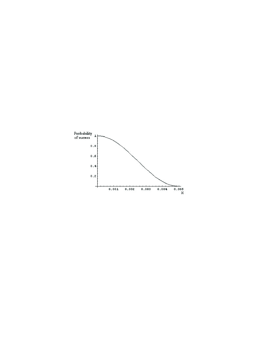
Figure 2: Probability of success to generate $|W^{gen}\rangle$ as function of $x=\frac{\delta}{t_{n}}$ in correspondence to $\Delta=0$ and n=100.

In figure 2 we plot the probability of success of our scheme given by eq. (16) versus $x=\frac{\delta}{t_{100}}$ putting $\Delta=0$ and $t=t_{100}+\delta$. As foreseeable, this probability of success remains of experimental interest for $x$ up to $3\cdot 10^{-3}$. Thus we may conclude that the procedure is stable enough against unavoidable uncertainties in the time instant at which the measurement of $\sigma_{z}^{A}$ is done.

Before concluding this section it is interesting to emphasize that the coupling between the $N$ spins and the central system generates entanglement between any two spins around the central one. In order to estimate the amount of such an entanglement and analyze its time evolution we evaluate the relative concurrence function. It is easy to prove that, starting from the initial state $|\psi_{0}(0)\rangle$, the reduced density $\rho_{ij}(t)$ describing the system of the two spins $i$ and $j$ among the $N$ uncoupled ones, can be written in the form

$$\rho_{ij}(t)=\left(\begin{array}[]{cccc}0&0&0&0\\ 0&|b_{i}(t)|^{2}&b_{i}(t)b_{j}(t)^{\ast}&0\\ 0&b_{i}(t)^{\ast}b_{j}(t)&|b_{j}(t)|^{2}&0\\ 0&0&0&|a(t)|^{2}+\sum_{k\neq i,j}|b_{k}(t)|^{2}\\ \end{array}\right)$$ (19)

when expressed in the standard two-spin basis $\{|\!\!\uparrow\uparrow\rangle,|\!\!\uparrow\downarrow\rangle,|\!\!\downarrow\uparrow\rangle,|\!\!\downarrow\downarrow\rangle\}$. In equation (19)$b_{j}(t)$ and $a(t)$ are given by eqs. (13) and (12) respectively. Thus the concurrence function $C_{ij}(t)$ turns out to be

$$C_{ij}(t)=\frac{2|\alpha_{i}||\alpha_{j}|}{\sum_{j=1}^{N}\alpha_{j}^{2}+\Delta^{2}}\sin^{2}\left(\sqrt{\sum_{j=1}^{N}\alpha_{j}^{2}+\Delta^{2}}\;t\right)$$ (20)

As expected, the degree of entanglement get established between the two uncoupled spins $i$ and $j$, oscillates with time $t$. In addition the maximum value of $C_{ij}(t)$ is proportional to $|\alpha_{i}||\alpha_{j}|$ and when $\alpha_{k}=\alpha$ $\forall k$ and $\Delta=0$ reaches the value $\frac{2}{N}$. This means that, increasing the number of spins around the central one, leads to a weak and weak pair quantum correlation in the system of interest.

4 Generation of well-defined angular momentum states of the N uncoupled spins

The W-state in eq.(15) is a multipartite entangled state of the $N$ uncoupled spins around the central one. On the other hand it coincides with a particular superposition of states in which $N-1$ spins have projection down while only one has projection up. This state can be thus obtained applying the collective ladder operator $\sigma_{+}=\sum_{i}\sigma_{+}^{(i)}$ on the state $|\!\!\downarrow,\downarrow,\ldots,\downarrow\rangle$ that is $|W\rangle\propto\sum_{i=1}^{N}\sigma_{+}^{(i)}|\!\!\downarrow,\downarrow,\ldots,\downarrow\rangle$. In other words the W-state is a common eigenstate of $\mathbf{J}^{2}$ and $J_{z}$, $\mathbf{J}=\frac{1}{2}\sum_{i=1}^{N}\mathbf{\sigma}_{i}$ being the collective angular momentum operator of the $N$ uncoupled spins, with

$$\mathbf{J}^{2}|W\rangle=\frac{N}{2}(\frac{N}{2}+1)|W\rangle$$ (21)

$$J_{z}|W\rangle=(-\frac{N}{2}+1)|W\rangle$$ (22)

Thus $|W\rangle\equiv|J,M\rangle$ whit $J=\frac{N}{2}$ and $M=-\frac{N}{2}+1$.

This observation suggests us the possibility to iterate our procedure in order to generate all the well defined angular momentum states $|J=\frac{N}{2},M\rangle$ with $M=-\frac{N}{2}\ldots\frac{N}{2}$.

Let’s indeed consider the spin star system in which the central spin interacts in the same way with all the others uncoupled $N$ spins, that is $\alpha_{j}\equiv\alpha\;\forall j$. Under this condition the hamiltonian model (1) is invariant by permutation of an arbitrary couple of spins among the $N$. Moreover $[\sigma^{A\,2},H]=[J^{2},H]=[\sigma_{z}^{A}+J_{z},H]=[J^{2}_{int},H]=0$, $\vec{J}_{int}$ being an intermediate angular momentum resulting from the coupling of selected at will individual angular momentum of the $N$ spins. These symmetry properties suggest to develop the dynamics of our system exploiting the coupled angular momentum basis $\{|J,M,\nu\rangle\}$ for the $N$ spins instead of the factorized one previously used. The index $\nu$ runs from 1 to $\nu_{MAX}(J)$ and allows us to distinguish between different states of the basis characterized by the same $J$ and $M$.

In the initial condition $|\psi_{0}(0)\rangle$ the $N$ spins around the central one are in the coupled angular momentum state $|J=\frac{N}{2},M=-\frac{N}{2},\nu=1\rangle$. In what follows we do not indicate anymore the the index $\nu$ remaining it equal to one. Thanks to the symmetry properties of our system at a generic time instant $t$ we can rewrite the state of the total system in the form

$$|\psi(t)\rangle=A_{1}(t)|\uparrow_{A}\rangle|\frac{N}{2},-\frac{N}{2}\rangle+B_{1}(t)|\downarrow_{A}\rangle|\frac{N}{2},-\frac{N}{2}+1\rangle$$ (23)

where

$$A_{1}=\cos(p_{1}\alpha t),$$ (24)

$$B_{1}=-i\sin(p_{1}\alpha t),$$ (25)

with

$$p_{1}=\sqrt{\frac{N}{2}\left(\frac{N}{2}+1\right)-\left(-\frac{N}{2}\right)\left(-\frac{N}{2}+1\right)}\equiv\sqrt{N}.$$ (26)

Thus as before, if we assume the central spin $A$ measured in the state $|\downarrow_{A}\rangle$ the $N$ uncoupled spins are projected onto the W-state $|W\rangle\equiv|\frac{N}{2},-\frac{N}{2}+1\rangle$. As demonstrated in the previous Section the probability of success to generate the W-state coincides with $\sin^{2}(p_{1}\alpha t)$ and it is equal to 1 if the measurement is performed at time instants $t_{n}=\frac{\pi(2n+1)}{2\alpha p_{1}}$ obtained from equation (17) putting $\alpha_{j}\equiv\alpha$ $\forall j$ and $\Delta=0$. Suppose now to iterate the procedure preparing once again the central spin in the up state. The new initial condition is then

$$|\psi(0)\rangle=|\uparrow_{A}\rangle|\frac{N}{2},-\frac{N}{2}+1\rangle$$ (27)

that as easily demonstrable evolves as

$$|\psi(t)\rangle=A_{2}(t)|\uparrow_{A}\rangle|\frac{N}{2},-\frac{N}{2}+1\rangle+B_{2}(t)|\downarrow_{A}\rangle|\frac{N}{2},-\frac{N}{2}+2\rangle$$ (28)

with

$$A_{2}(t)=\cos(p_{2}\alpha t)$$ (29)

$$B_{2}(t)=-i\sin(p_{2}\alpha t)$$ (30)

where $p_{2}=\sqrt{\frac{N}{2}(\frac{N}{2}+1)-(-\frac{N}{2}+1)(-\frac{N}{2}+2)}$. Eq. (28) immediately implies that, measuring the spin $A$ in its down state, makes the $N$ spins to collapse onto the angular momentum state $|\frac{N}{2},-\frac{N}{2}+2\rangle$. It is possible at this point to convince oneself that, iterating $k$-times our procedure, we generate the coupled angular momentum state $|\frac{N}{2},-\frac{N}{2}+k\rangle$. As far as the probability of success $P_{k}$ that after $k$ measurements the $N$ uncoupled spins are left in the state $|\frac{N}{2},-\frac{N}{2}+k\rangle$, it is easy to prove that it is given by

$$P_{k}=\prod_{i=1}^{k}\sin^{2}(p_{i}\alpha t)$$ (31)

where $p_{i}=\sqrt{\frac{N}{2}(\frac{N}{2}+1)-(-\frac{N}{2}+i-1)(-\frac{N}{2}+i)}$.

Thus, if at the $i-$th step we have the possibility of choosing the time instant at which performing the measurement act on the central spin $A$ in such a way that $t_{n}^{(i)}=\frac{(2n+1)\pi}{2\alpha p_{i}}$, at least in principle we may claim that the desired state $|\frac{N}{2},-\frac{N}{2}+k\rangle$ of the $N$ spins are generated with certainty.

5 Estimating the order of magnitude of the coupling constant $\alpha_{j}$

As we are going to prove the dynamics of our system can be also successfully exploited in order to estimate the coupling intensity between each of the $N$ distinguishable and non interacting $N$ spins and the central one.

Let’s indeed consider for simplicity the case $\Delta=0$ and, under this condition, concentrate on the behaviour of the probability $P_{0}(t)$ to find the system, at a generic time instant $t$, in the initial condition $|\psi_{0}(0)\rangle$. The results obtained in the previous Section immediately implies that such a probability is given by

$$P_{0}(t)=|a(t)|^{2}=\cos^{2}\left(\sqrt{\sum_{j=1}^{N}\alpha_{j}^{2}}\;t\right).$$ (32)

Thus, the probability of recovering the $N$ uncoupled spins as well as the central one in their initial state is a periodic function of $t$, the period being in inverse relation to the quantity $\sum_{j=1}^{N}\alpha_{j}^{2}$. If, as reasonable, we assume that all the coupling constants are of the same order, analyzing the temporal behaviour of $P_{0}(t)$, we have the possibility of estimating the order of magnitude of each $\alpha_{j}$. It is important to stress that the possibility of knowing at least the order of magnitude of the coupling constants $\alpha_{j}$ play a central role for example in all the cases in which the spin of an electron localized in a quantum dot is used as realization of a quantum bit Merkulov . In these cases indeed the spin relaxation mechanism is mainly connected with its interaction with bulk nuclear spins.

Let’s moreover observe that the knowledge of the frequency of the function $P_{0}(t)$ given by eq. (32) can be also exploited in order to estimate how much disordered the spin star system model (1) is. Let’s suppose indeed that the $N$ spins of interest have been prepared in a W-like state following the procedure previously discussed. At this point, if we measure the observable $\sigma_{z}^{j}$ finding the eigenvalue $+1$, then the total system is projected onto the state $|\!\!\downarrow,\downarrow,\ldots,\uparrow_{j},\ldots,\downarrow\rangle$ in which only the $j$-th spin is in its upper state whereas the others are in their respective down state. The probability of such an event, directly obtainable starting from eq.(14), exactly coincides with the quantity $\frac{\alpha_{j}^{2}}{\sum_{j=1}^{N}\alpha_{j}^{2}}$.

We may thus conclude that knowing the probability of success to find the $j$-th spin in the up state $|\!\!\uparrow\rangle$ when the system of $N$ spins is prepared in a W-like state, allows us to give an estimation of the interaction strength between the $j$-th spin and the central one.

6 Conclusion

Generally speaking the possibility of establishing on demand fixed entanglement conditions in a multipartite system is an interesting objective both in its own and also in view of its applicative potentialities. In this paper in particular we have concentrated on a multipartite system composed by $N$ not interacting spins $\frac{1}{2}$. In order to guide this system toward assigned entangled states, we have exploited the interaction between each of the $N$ subsystems with a single spin $\frac{1}{2}$. The disordered spin star system thus obtained has been successfully used to generate W-like states as well as well-defined angular momentum states of the $N$ uncoupled spins.

The study of the exact dynamics of the disordered spin star system reported in this paper, has provided the possibility to envisage a way to estimate at least the order of magnitude of the coupling strength between each of the $N$ uncoupled spins and the central one. To gain this information is, for example, of particular relevance when electron spin relaxation plays an important role. It is indeed appropriate to remark that our system can be adopted to describe hyperfine interaction of a single electron spin with nuclei in quantum dots and that this interaction mechanism may be the dominant source of electron spin relaxation.

References

- (1) A. Bayat, S. Bose, quant-ph/07064176 (2007)
- (2) V. Kostak, G. M. Nikolopoulos, I. Jex, quant-ph/0702016 (2007)
- (3) M. B. Plenio, S. Virmani, quant-ph/0702059 (2007)
- (4) J. S. Pratt, Phys. Rev. A , 042312 (2004)
- (5) G.L. Kamta, A. Starace, Phys. Rev. Lett. , 10 (2002)
- (6) S. Hamieh, M.I. Katsnelson, Phys. Rev. A , 032316 (2005)
- (7) P. Karbach, J. Stolze, Phys. Rev. A , 030301 (2005)
- (8) D. Bruß, N. Datta, A. Ekert, L. C. Kwek, C. Machiavello, Phys. Rev. A , 014301 (2005)
- (9) V. Subrahmanyam, Phys. Rev. A , 034304 (2004)
- (10) F. Pan, X. Guan, N. Ma, W.-J. Han, J. P. Draayerb, quant-ph/0702030 (2007)
- (11) A. Hutton, S. Bose, Phys. Rev. Lett. , 237205 (2004)
- (12) X.-Z. Yuan,H.-S. Goan, K.-D. Zhu, Phys. Rev. B , 045331 (2007)
- (13) Y. Hamdouni, M. Fannes, F. Petruccione, Phys. Rev. B , 245323 (2006)
- (14) Jan Fischer, H-P Breuer quant-ph 0708.0410v1 (2007)
- (15) F. Verstraete, M. Popp, J.I. Cirac, Phys. Rev. Lett. , 027901 (2004)
- (16) M.C. Arnesen, S. Bose, V. Vedral, Phys. Rev. Lett. , 017901 (2001)
- (17) J.S. Pratt, Phys. Rev. Lett. , 237205 (2004)
- (18) D. Binosi, G. De Chiara, S. Montangero, A. Recati, cond-math 0707.0266v2 (2007)
- (19) D.D. Braktavatsala Rao, V. Ravishankar, V. Subrahmanyam, Phys. Rev. A , 022301 (2006)
- (20) J. Schliemann, A. V. Khaetskii, D. Loss, Phys. Rev. B , 245303 (2002)
- (21) R. Horodecki, P. Horodecki, M. Horodecki, K. Horodecki, quant-ph/0702225 (2007)
- (22) I.A. Merkulov, A.L. Efros, M. Rosen, Phys. Rev. B , 205309 (2002)
- (23) D.C. Mattis, The theory of magnetism made simple, World Scientific (2006)