Hartree-Fock Interactions in the Integer Quantum Hall Effect

Abstract.

We report on numerical studies into the interplay of disorder and electron-electron interactions within the integer quantum Hall regime, where the presence of a strong magnetic field and two-dimensional confinement of the electronic system profoundly affects thermodynamic and transport properties. We emphasise the behaviour of the electronic compressibility, the local density of states, and the Kubo conductivity. Our treatment of the electron-electron interactions relies on the Hartree-Fock approximation so as to achieve system sizes comparable to experimental situations. Our results clearly exhibit manifestations of various interaction-mediated features, such as non-linear screening, local charging, and $g$-factor enhancement, implying the inadequacy of independent-particle models for comparison with experimental results.

1. Introduction

The integer quantum Hall effect (IQHE) — observed in two-dimensional electron systems (2DES) subject to a strong perpendicular magnetic field [1] — has been well studied using single-particle arguments [2, 3, 4, 5, 6, 7, 8, 9, 10, 11]. However, experiments on mesoscopic MOSFET devices have questioned the validity of such a simple single-particle picture. Measurements of the Hall conductance as a function of magnetic field $B$ and gate voltage [12] exhibited regular patterns along integer filling factors. It was argued that these patterns should be attributed to Coulomb blockade effects. Similar patterns have been found recently also in measurements of the electronic compressibility $\kappa$ as a function of $B$ and electron density $n_{\rm e}$ in the IQHE [13] as well as the fractional quantum Hall effect (FQHE) [14]. From these measurements it turns out that deep in the localised regime between two Landau levels, stripes of constant width with particularly small $\kappa$ can be identified. These stripes consist of a collection of small-$\kappa$ lines, identifiable with localised states, and their number is independent of $B$. This is inconsistent with a single-particle picture where one expects a fan-diagram of lines emanating from $(0,0)$ in the $(B,n_{\rm e})$-plane. The authors of [13, 14] argue that their results may be explained qualitatively by non-linear screening of the impurity charge density at the Landau level band edges. Clearly, such screening effects — described within a Thomas-Fermi approach [13] — are beyond the scope of a non-interacting theory. This immediately raises a question on the status of the aforementioned universality of the QH transition [12, 15, 16], which was obtained largely within a single-particle approach [17, 9, 18, 19, 20, 21, 22, 23]. Indeed a recently developed theory of the IQHE for short-ranged disorder and Coulomb interactions shows that universality is retained due to $\mathcal{F}$ invariance [24, 25, 26].

In the present paper, we quantitatively investigate the effects of Coulomb interactions on the compressibility in the $(B,n_{\rm e})$-plane within a Hartree-Fock (HF) approach. HF accounts for Thomas-Fermi screening effects while at the same time leading to a critical exponent $\nu$ whose value is consistent with the results of the non-interacting approaches [27, 28, 29]. We find that the observed charging lines in the compressibility can be well reproduced and that the width of each group of lines is well estimated by a force balance argument. Thus we can quantitatively explain the lines and stripes in the compressibility as a function of $(B,n_{\rm e})$, fully in support of the qualitative picture proposed in [13, 30, 31, 32]. However, our results for the conductivity patterns of Ref. [12] do not seem to reproduce the observed stripes. This might be due to our still too small system sizes [33] or many-particle physics beyond the HF approximation [34].

2. The Hartree-Fock approach in Landau basis

We consider a 2DES in the $(x,y)$-plane subject to a perpendicular magnetic field ${\mathbf{B}}=B{\mathbf{e}}_{z}$. The system can be described by a Hamiltonian of the form

$$H^{\sigma}_{\rm 2DES}=h^{\sigma}+V_{\rm C}=\frac{({\mathbf{p}}-e{\mathbf{A}})^{2}}{2m^{*}}+\frac{\sigma g^{*}\mu_{\rm B}B}{2}+V_{\rm I}({\mathbf{r}})+V_{\rm C}({\mathbf{r}},{\mathbf{r}}^{\prime}),$$ (1)

where $\sigma=\pm 1$ is a spin degree of freedom, $V_{\rm I}$ is a smooth random potential modelling the effect of the electron-impurity interaction, $V_{\rm C}$ represents the electron-electron interaction term and $m^{*}$, $g^{*}$, and $\mu_{\rm B}$ are the effective electron mass, $g$-factor, and Bohr magneton, respectively [35].

The electron-electron interaction potential has the form

$$V_{\rm C}({\mathbf{r}},{\mathbf{r}}^{\prime})=\frac{e^{2}}{4\pi\epsilon\epsilon_{0}}\frac{\gamma}{|{\mathbf{r}}-{\mathbf{r}}^{\prime}|}=\sum_{{\mathbf{q}}}V_{\rm C}({\mathbf{q}})\exp\left[{i}{\mathbf{q}}\cdot({\mathbf{r}}-{\mathbf{r}}^{\prime})\right],$$ (2)

with

$$V_{\rm C}({\mathbf{q}})=\frac{e^{2}}{4\pi\epsilon\epsilon_{0}l_{\rm c}}\frac{\gamma}{N_{\phi}|{\mathbf{q}}|l_{\rm c}}.$$ (3)

The parameter $\gamma$ will allow us to continually adjust the interaction strength; $\gamma=1$ corresponds to the bare Coulomb interaction. Using $\gamma<1$ merely serves as a numerical handle to the interaction strength and might be easily eliminated by rescaling of the disorder strength. $N_{\phi}=L^{2}/2\pi l_{c}^{2}$ is the number of states per Landau level, also referred to as the number of magnetic flux quanta. Choosing the vector potential in Landau gauge, ${\mathbf{A}}=Bx{\mathbf{e}}_{y}$, the kinetic part of the Hamiltonian is diagonal in the Landau functions [36]

$$\varphi_{n,k}({\mathbf{r}})=\langle{\mathbf{r}}|nk\rangle=\frac{1}{\sqrt{2^{n}n!\sqrt{\pi}l_{\rm c}L}}\exp\left[{i}ky-\frac{(x-kl_{\rm c}^{2})^{2}}{2l_{\rm c}^{2}}\right]H_{n}\left(\frac{x-kl_{\rm c}^{2}}{l_{\rm c}}\right),$$ (4)

where $n$ labels the Landau level index, $k={2\pi j}/{L}$ with $j=0,\ldots,N_{\phi}-1$ labelling the momentum, $H_{n}(x)$ is the $n$th Hermite polynomial, and $l_{\rm c}=\sqrt{\hbar/eB}$ the magnetic length. We use $N_{\rm I}$ Gaussian-type ”impurities”, randomly distributed at ${\mathbf{r}}_{s}$, with random strengths $w_{s}\in[-W,W]$, and a fixed width $d$, such that $V_{\rm I}({\mathbf{r}})=\sum_{s=1}^{N_{\rm I}}\left(w_{s}/\pi d^{2}\right)\exp[-({\mathbf{r}}-{\mathbf{r}}_{s})^{2}/d^{2}]=\sum_{{\mathbf{q}}}V_{\rm I}({\mathbf{q}})\exp({i}{\mathbf{q}}\cdot{\mathbf{r}})$ with

$$V_{\rm I}({\mathbf{q}})=\sum_{s=1}^{N_{\rm I}}\frac{w_{s}}{L^{2}}\exp\left(-\frac{d^{2}|{\mathbf{q}}|^{2}}{4}-{i}{\mathbf{q}}\cdot{\mathbf{r}}_{s}\right),$$ (5)

where $q_{x,y}={2\pi j}/{L}$ and $j=-N_{\phi},-N_{\phi}-1,\ldots,N_{\phi}$. The areal density of impurities therefore is given by $n_{\rm I}=N_{\rm I}/L^{2}$. The Hamiltonian is represented in matrix form using the periodic Landau states $|nk\rangle$ and we have

$$\mathbf{H}^{\sigma}_{n,k;n^{\prime},k^{\prime}} = \langle nk|H^{\sigma}_{\rm 2DES}|n^{\prime}k^{\prime}\rangle$$ (6)

$$= \left(n+\frac{1}{2}+\frac{\sigma g^{*}}{4}\frac{m^{*}}{m_{\rm e}}\right)\hbar\omega_{\rm c}\delta_{n,n^{\prime}}\delta_{k,k^{\prime}}+\mathbf{V}_{n,k;n^{\prime},k^{\prime}}+\mathbf{F}^{\sigma}_{n,k;n^{\prime},k^{\prime}}\quad,$$

with the cyclotron energy $\hbar\omega_{\rm c}=\hbar eB/m^{*}$. The disorder matrix elements are given by $\mathbf{V}_{n,k;n^{\prime},k^{\prime}}=\sum_{{\mathbf{q}}}V_{\rm I}({\mathbf{q}})S_{n,k;n^{\prime},k^{\prime}}({\mathbf{q}})$, where mixing of Landau levels is included. The explicit form of the plane wave matrix elements $S_{n,k;n^{\prime},k^{\prime}}({\mathbf{q}})=\langle nk|\exp({i}{\mathbf{q}}\cdot{{\mathbf{r}}})|n^{\prime}k^{\prime}\rangle$ and the Fock matrix $\mathbf{F}^{\sigma}_{n,k;n^{\prime},k^{\prime}}$ can be found in Ref. [29]. The total energy $E_{\rm tot}$ in terms of the above matrices is given as

$$E_{\rm tot}=\mbox{Tr}(\mathbf{h}\mathbf{D}+\frac{1}{2}\mathbf{F}\mathbf{D})=\frac{1}{2}\sum_{\sigma}\sum_{n,k;n^{\prime},k^{\prime}}\left(2\mathbf{h}^{\sigma}_{n,k;n^{\prime},k^{\prime}}+\mathbf{F}^{\sigma}_{n,k;n^{\prime},k^{\prime}}\right)\mathbf{D}^{\sigma}_{n^{\prime},k^{\prime};n,k}$$ (7)

where the density matrix is $\mathbf{D}_{n,a;m,b}=\sum_{\alpha}f_{\alpha}C^{\alpha}_{n,a}C^{\alpha,*}_{m,b}$ with $f_{\alpha}$ the Fermi function and $C_{n,a}^{\alpha}$ the expansion coefficients for the Landau basis [29]. The sums $n$ and $n^{\prime}$ run over the number of Landau levels, $N_{\rm LL}$, taken into account. A variational minimisation of $\langle\Psi|H_{\rm 2DES}|\Psi\rangle$ with respect to the coefficients yields the Hartree-Fock-Roothaan equation [37]. The simplest scheme for solving this self-consistent eigenvalue problem is the Roothaan algorithm [37, 38]. However, convergence of the Roothaan algorithm is rather poor. In most cases it runs into an oscillating limit cycle [35]. This limit cycle can be avoided be minimising a penalised energy functional

$$E^{\prime}(\mathbf{D}_{\rm old},\mathbf{D}_{\rm new})=E(\mathbf{D}_{\rm old},\mathbf{D}_{\rm new})+b||\mathbf{D}_{\rm old}-\mathbf{D}_{\rm new}||^{2}~{},$$ (8)

instead of the actual HF energy functional where “old” and “new“ denote two consecutive states in the HF-selfconsistency cycle. This then leads to the Level-Shifting algorithm (LSA) [39]. However, while LSA avoids limit cycles, it can and does lead to unphysical solutions. A further improvement is based on the Optimal-Damping algorithm (ODA) [38]. The iteration is carried out just as in the Roothaan algorithm, only that the new density matrix is a mixture of the old and the new density matrix, i.e.

$$\mathbf{D}=(1-\lambda)\mathbf{D}_{\rm old}+\lambda\mathbf{D}_{\rm new}~{},$$ (9)

with a damping parameter $\lambda$ which is chosen optimally according to the direction of steepest descent in the total HF energy [35]. As it turns out the performance also depends strongly on the interaction strength and the position of the Fermi level. For some filling factors and choices of parameters, we might find fast convergence with one of the algorithms described above. However, over the whole range of filling factors only a combination of ODA and LSA can guarantee convergence in any case. In Fig. 1 we have depicted the convergence behaviour for a typical HF run at four different filling factors. Note that we have plotted the convergence as defined by Eq. (8), rather than the total HF energy, which is also sometimes used as a measure. In comparison to the energy which acquires a finite value at convergence, the error estimate $||\mathbf{D}_{\rm new}-\mathbf{D}_{\rm old}||$ goes to zero and its convergence is therefore easier to interpret.

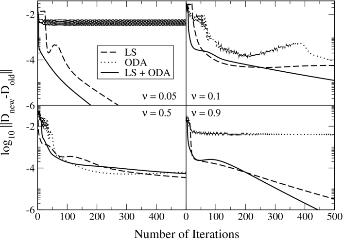
Figure 1. Dependence of the convergence on the number of HF iterations for the three HF algorithms. The four panels correspond to $4$ different filling factors.

3. Wave function and charge distributions

3.1. The local density of states

The local density of states (LDOS) is a very interesting quantity which is experimentally accessible via spatial scanning tunneling spectroscopy (STS) [40, 41, 42]. The differential tunneling current between the STS tip and the sample is thereby proportional to the density of existing states at a certain energy. By definition the LDOS is the tunneling density of states (TDOS) weighted with the charge density at a position ${\mathbf{r}}$, defined by

$$\mbox{LDOS}(E,{\mathbf{r}})=\sum_{\alpha}|\psi_{\alpha}({\mathbf{r}})|^{2}\delta(E-E_{\alpha})~{},$$ (10)

such that $\int d^{2}{\mathbf{r}}\mbox{LDOS}(E,{\mathbf{r}})=\sum_{\alpha}\delta(E-E_{\alpha})=\rho(E)$, where $\rho(E)$ is the TDOS. In practice, the $\delta$-function is broadened by temperature as well as an AC modulation voltage applied when using a lock-in technique for noise reduction. The energy window can then be described by a semi-ellipse around $E$ with the broadening $\Delta E$, which is usually of the order of $1$meV [41]. Thus, the LDOS can be regarded as the charge density in a small energy interval and allows to study the charge distribution in the 3 dimensions (2 spatial and energy).

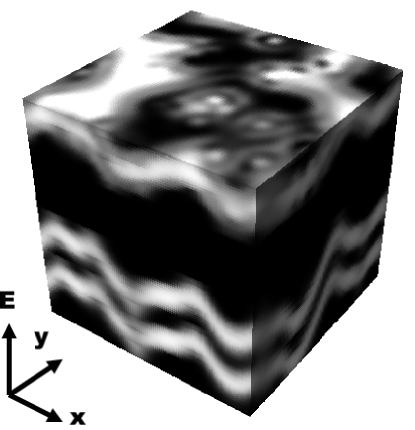
Figure 2. Local density of states for a non-interacting Hall system as a function of $(x,y)$ position as well as energy $E$ for a system of size $L=300nm$. The filling factor $\nu\approx 3$ and $B=5$T. Large LDOS values are indicated by white.

In Figs. 2 and 3 we show results for a model of an n-type InSb structure of three-dimensionally distributed donor atoms with a 2DES sitting on top of the cleaved surface [42]. The first $2$ spin-split Landau levels are shown for Fig. 3. At filling factor $\nu=0$, electrons are tunneling from the tip into unoccupied states of the sample and one thus probes non-interacting physics. A spin-splitting equal to the Zeeman energy can be seen which is of equal magnitude in each level. In the right panel of Fig. 3, we show the situation at $\nu=0.5$, i.e. when the Fermi energy lies right in the centre of the lowest Landau level.

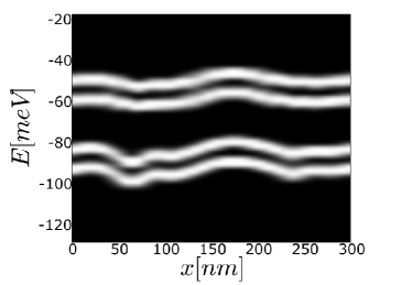
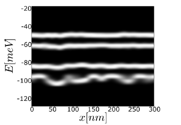
Figure 3. Local density of states as a function of $x$ position as well as energy $E$ for a system of size $L=300nm$ at constant $y$ and $B=5$T. The filling factor $\nu=0$ (left) and $\nu=0.5$ (right). Large LDOS values are indicated by white.

We observe that the high-LDOS features of this level appear to be pushed away from the Fermi energy, resulting in the onset of the famous Coulomb gap (”Efros-Shklovskii gap”, see [43]) in the TDOS. We would like to note that the gap in the TDOS shall not be confused with the gaps appearing in the quasi-particle spectrum. In fact, it has been shown that despite the linear Coulomb gap in the TDOS, the thermodynamic density of states remains finite at the Fermi level [44, 29]. Furthermore, the fluctuations in this level are much stronger than in the other three levels. We interpret this as a signature of the screening mechanism, i.e. the electrons near the Fermi level screen the disorder such that the states in the higher levels only see a weakened disorder potential. We also see that the spin-splitting in the first level is enhanced as compared to the non-interacting case. Similarly, the spin-splitting between levels $3$ and $4$ is also larger. These effects seems to be related to the direct and indirect spin splitting enhancements for instance recently reported in Ref. [33].

3.2. The charge distribution

The spatial distribution of the total electronic density

$$n({\mathbf{r}})=\sum_{\sigma}\sum_{\alpha=1}^{M}\left|\psi_{\alpha}^{\sigma}({\mathbf{r}})\right|^{2}=L^{-2}\sum_{\sigma}\sum_{n,k,n^{\prime},k^{\prime}}\sum_{{\mathbf{q}}}\mathbf{D}^{\sigma}_{n,k;n^{\prime},k^{\prime}}S_{n,k;n^{\prime},k^{\prime}}({\mathbf{q}})\exp(-{i}{\mathbf{q}}{\mathbf{r}})$$ (11)

is also readily calculated in our approach. It details the screening mechanism by providing direct insight into the interplay of disorder and interaction. Let us start at the QH transition. Fig.  4 depicts the critical charge density at $\nu=1/2$ for a non-interacting system in units of $n_{0}$.

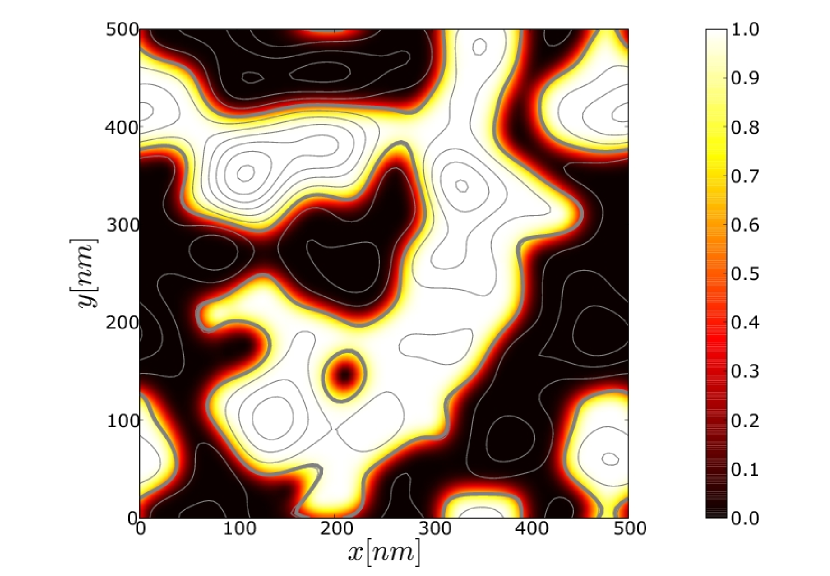
Figure 4. Spatial distribution of non-interacting electron density $n({\mathbf{r}})/n_{0}$ at $B=4$T, $\gamma=0$ and $\nu=1/2$ as indicated by the colour scale. Solid contour lines show the equipotential lines of the $V_{\rm I}({\mathbf{r}})$. The thick solid lines corresponds to $\epsilon_{\rm F}$.

The contour lines show the impurity potential $V_{\rm I}({\mathbf{r}})$ where the critical energy $V_{\rm I}({\mathbf{r}})=\epsilon_{\rm F}$ is highlighted by a thick line. The charge density evidently behaves according to the semiclassical approximation [21] and follows the equipotential lines of $V_{\rm I}({\mathbf{r}})$. For the interacting case, however, we expect Thomas-Fermi screening theory to apply [45, 46, 47, 48]. This approximation is appropriate for an impurity potential smooth on the scale of the magnetic length as well as a sufficient separation of the Landau bands, characterised by the condition $\hbar\omega_{\rm c}/l_{\rm c}>\sqrt{\langle|\nabla V_{\rm I}({\mathbf{r}})|^{2}\rangle}$. The induced electrostatic potential of the charge density

$$\phi({\mathbf{r}})=\frac{e}{4\pi\epsilon\epsilon_{0}}\int d^{2}{\mathbf{r}}^{\prime}\frac{n({\mathbf{r}}^{\prime})-\bar{n}}{|{\mathbf{r}}^{\prime}-{\mathbf{r}}|}$$ (12)

and the impurity potential $V_{\rm I}({\mathbf{r}})$ form a screened potential $V_{\rm scr}({\mathbf{r}})=V_{\rm I}({\mathbf{r}})+e\phi({\mathbf{r}})$. Here, $\bar{n}$ accounts for the positive background. Since a flat screened potential is energetically most favourable, one expects to find $V_{\rm scr}({\mathbf{r}})=\epsilon_{\rm F}$ for the case of perfect screening. However, since fluctuations of the charge density, $n({\mathbf{r}})$, are restricted between an empty and a full Landau level, i.e. $(N_{\rm LL}-1)n_{0}<n({\mathbf{r}})<N_{\rm LL}n_{0}$, where $n_{0}=(2\pi l_{c}^{2})^{-1}$ is the density of a full Landau level, the screening is not always perfect but depends on the fluctuations in the impurity potential as well as on the filling factor [45, 46, 47]. With the condition that $\hbar\omega_{c}$ is large compared to the potential energy scale, we can restrict the discussion to a single Landau level, i.e. $N_{\rm LL}=1$. The plane can be divided into fully electron or hole depleted, insulating regions — where $n({\mathbf{r}})=0$ or $n({\mathbf{r}})=n_{0}$, respectively — and metallic regions — where $n({\mathbf{r}})$ lies in between. Depending on the filling factor, the extent of those regions varies. Close to the band edge, insulating regions dominate. Screening is highly non-linear and transport virtually impossible. On the other hand, if disorder is weak enough, there exists a finite range of filling factors in the centre of each band where metallic regions cover most of the sample, percolate and render the whole system metallic. The disorder is effectively screened and transport greatly enhanced. In that case, the charge density $n_{\rm scr}({\mathbf{r}})$ can be obtained by Fourier transforming the screened potential. In 3D, this simply leads to the Laplace equation. For 2D [49], however, one obtains $n_{\rm scr}({\mathbf{q}})=-(2\epsilon\epsilon_{0}/e^{2})|{\mathbf{q}}|V_{\rm I}({\mathbf{q}})+\nu n_{0}\delta_{q,0},$where the $|{\mathbf{q}}|=0$ only couples to the homogeneous, positive background and thus does not contribute to screening of the impurity potential. In other words, in our model only the fluctuations $\delta n({\mathbf{{\mathbf{r}}}})$ are essential for screening. Hence, in 2D, a perfectly screening charge density would obey

$$n_{\rm scr}({\mathbf{r}})=-\frac{4\pi\epsilon\epsilon_{0}}{e^{2}}\int d^{2}{\mathbf{r}}^{\prime}\frac{\Delta_{\rm 2D}V_{\rm I}({\mathbf{r}}^{\prime})}{|{\mathbf{r}}-{\mathbf{r}}^{\prime}|}+\nu n_{0}.$$ (13)

Clearly, the actual charge density is expected to deviate from $n_{\rm scr}({\mathbf{r}})$ for several reasons. Firstly, the fluctuations of $n({\mathbf{r}})$ are restricted as discussed above. Secondly, (13) is valid for the Hartree case only. Taking the Fock contribution into account will introduce short wavelength fluctuations due to the tendency for crystallization. Fig. 5 shows results for the charge density of interacting electrons at $\nu=0.5$. Broken lines indicate the regions where $n_{\rm scr}({\mathbf{r}})$ exceeds the range for $\delta n({\mathbf{r}})$ either below or above, i.e. areas that cannot be screened at all and thus exhibit insulating behaviour.

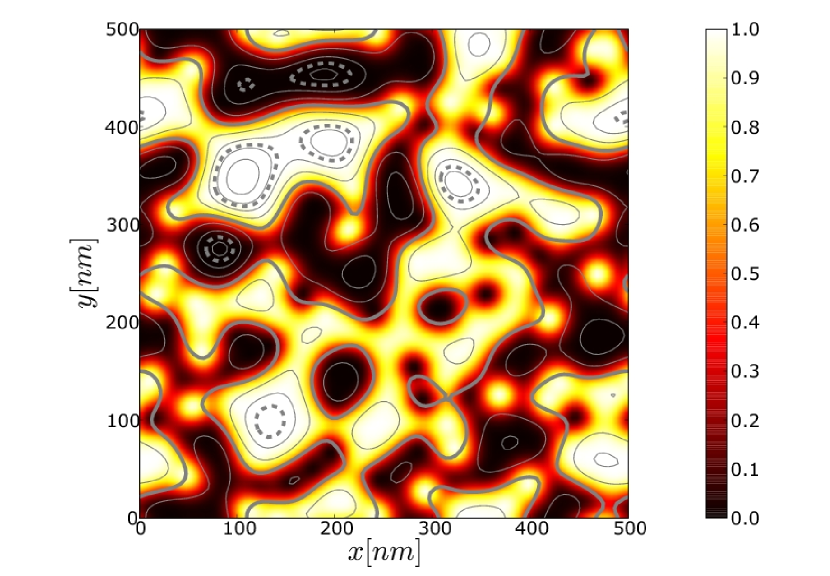
Figure 5. Spatial distribution of HF-interacting electron density $n({\mathbf{r}})/n_{0}$ at $B=4$T, $\gamma=0.3$ and $\nu=1/2$ as indicated by the colour scale. Contour lines show equidensity lines of (13). The broken lines indicate unscreenable (insulating) regions. The thick solid line shows $n_{\rm scr}({\mathbf{r}})=\bar{n}_{\rm scr}=0$.

Otherwise, we find the charge density to follow $n_{\rm scr}({\mathbf{r}})$ very closely. In this regime, the density is well described by (13) and the screening is very effective. Metallic regions dominate over insulating ones and transport is expected to be good.

We hence have established that interactions at the level of HF already give rise to substantial differences in the LDOS and local charge density distributions. Thus one might wonder why theoretical models based on non-interacting charges work at all. However, comparing Figs. 4 and 5 side by side, we see that the charge density, following the percolating equipotential at half filling for the non-interacting Fig. 4, retains many of the properties of the HF-interacting charge density line given by $n_{\rm scr}({\mathbf{r}})=\bar{n}_{\rm scr}=0$. Thus non-interacting percolation-type arguments for network models [9, 23, 11] should indeed provide a good starting point for a qualitative description of the QH transition.

4. Compressibilities and Coulomb blockade

In order to understand the experimental results [13, 14] we need to focus on the physics of the 2DES near the Landau band edges. As opposed to the band centre, in this regime the measured compressibility exhibits very strong fluctuations as a function of electron density which is due to sharp jumps in the chemical potential upon varying the carrier density. A clearer picture of what the microscopic situation is can be obtained by a spatially resolved scan of $\kappa^{-1}$. Unlike the fixed-position $(B,n_{\rm e})$-scans, the SET tip will thereby pick up the spatial variations of the chemical potential change. In the measurements of Ilani and coworkers [13], spatially localised jumps of the chemical potential are clearly identifiable which form bent segments within the $(x,n_{\rm e})$-plane. These jumps are fingerprints of local charge accumulation and allow to conclude that quantum-dot-like structures of electrons (near an empty Landau band) or holes (near a full Landau band) must be formed within the sample. The multitude of lines in the compressibility originating from the dots are indications of Coulomb blockade effects and provide information on the position, charging as well as spatial extent of the dots. Since the charge is confined to a small region within the sample, Coulomb repulsion amongst the particles requires a comparably large amount of energy for adding or removing an electron to or from the dot. An increase in the number of electrons is thus accompanied by equidistant jumps in the chemical potential. The bending of the compressibility patterns is a feature of the SET tip bias which acts as an additional potential at the tip site. As the tip scans across a particular dot, it affects its charging condition as a function of distance to the centre which results in the observed arc-like distortion.

Now we want to investigate whether our model is capable of producing dot spectra as found in the experiment. The change of the local chemical potential with respect to the electron density can be computed for our system by noting that the local chemical potential is the functional derivative of the total energy with respect to the spatial electron density

$$\mu({\mathbf{r}})=\frac{\delta E_{\rm tot}[n]}{\delta n({\mathbf{r}})}=\frac{\delta}{\delta n({\mathbf{r}})}\iint d^{2}{\mathbf{r}}d^{2}{\mathbf{r}}^{\prime}\frac{n({\mathbf{r}})n({\mathbf{r}}^{\prime})}{|{\mathbf{r}}-{\mathbf{r}}^{\prime}|}=\int d^{2}{\mathbf{r}}^{\prime}\frac{n({\mathbf{r}}^{\prime})}{|{\mathbf{r}}-{\mathbf{r}}^{\prime}|}~{}.$$ (14)

Hence, we confirm the anticipated results that the chemical potential is simply the electrostatic potential due to the electrons in the 2DES. In terms of our previous definitions, the electrostatic potential of the 2DES reads

$$\phi({\mathbf{r}})=L^{-2}\sum_{\sigma}\sum_{n,k,n^{\prime},k^{\prime}}\sum_{{\mathbf{q}}}V_{\rm C}({\mathbf{q}})\mathbf{D}^{\sigma}_{n,k;n^{\prime},k^{\prime}}S_{n,k;n^{\prime},k^{\prime}}({\mathbf{q}})\exp(-{i}{\mathbf{q}}{\mathbf{r}})$$ (15)

and the local inverse electronic compressibility can be evaluated as

$$\kappa^{-1}({\mathbf{r}})\propto\mu^{N+1}({\mathbf{r}})-\mu^{N}({\mathbf{r}})\propto\phi^{N+1}({\mathbf{r}})-\phi^{N}({\mathbf{r}}).$$ (16)

We have calculated $\kappa^{-1}({\mathbf{r}})$ for the lowest two Landau levels for a system of size $L=500$nm without spin as a function of position and carrier density at magnetic field $B=2$T. The SET tip potential, $V_{\rm Tip}({\mathbf{r}})$, has been approximated by a Gaussian function $V_{\rm Tip}({\mathbf{r}})={w_{\rm Tip}}/{\pi d_{\rm Tip}^{2}}\exp[{-({\mathbf{r}}-{\mathbf{R}}_{\rm Tip})^{2}/d_{\rm Tip}^{2}}]$ with $w_{\rm Tip}=6$meV and $d_{\rm Tip}=5$nm. The sample is then ”probed” along the $x$-axis at ${\mathbf{R}}_{\rm Tip}=(i/50)L$, where $i=1,\dots,50$. For each position of the tip the total potential has to be evaluated and a complete HF run is carried out since the tip affects the electron density at each position differently. The results are presented in Fig.  6.

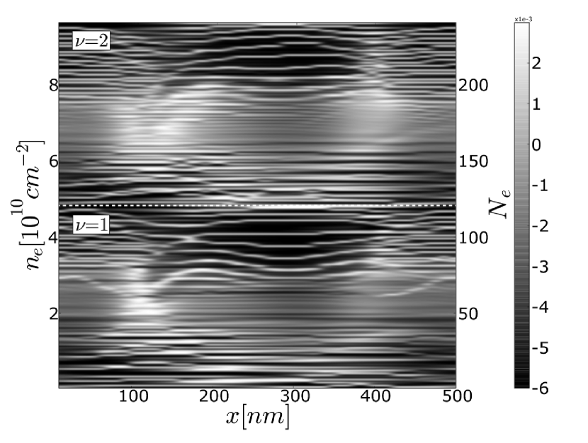
Figure 6. Inverse electronic compressibility $\kappa^{-1}$ for a HF-interacting system of size $L=500$nm as a function of position $x$ and electron density $n_{\rm e}$ in the two lowest Landau levels without spin. The $y$ coordinate has been fixed at $250$nm. The patterns correspond to jumps in the chemical potential due to charging of local charge puddles (see text for details).

We find remarkable agreement with the experimental results. Distinct charging patterns appear at the Landau band edges, whereas in the centre of the bands the features are much weaker. Thus, we have shown that our model is able to exhibit Coulomb blockade patterns. We consequently also expect the $(B,n_{\rm e})$-calculations to exhibit charging patterns similar to the experimental results and indeed in Ref. [29] we show good agreement between our model and the results of Ref. [13, 14].

5. Interaction effects in the Hall conductivity

The compressibility patterns found in the experiments discussed above were preceded by transport experiments that revealed patters in the conductance, also clearly interaction mediated. Cobden et al. [12] reported on Hall conductance measurements on mesoscopic MOSFET devices in the $(V_{\rm g},B)$-plane, where $V_{\rm g}$ is the gate voltage, that displayed a contradictive behaviour to the expectations deduced from a single-particle model. The gate voltage $V_{\rm g}$ can be linked to the electron number density as $dn_{\rm e}/dV_{\rm g}=C/e$, where $C$ is a material specific constant. A line in the $(V_{\rm g},B)$-plane originating from $V_{\rm g}(n_{\rm e}=0)$ can thus be labeled by a certain filling factor $\nu$.

The fluctuations around the plateau transitions found in Ref. [12] at half integer filling factor are apparently correlated over a large interval of the magnetic field. Surprisingly, however, the lines formed by the conductance extrema in the $(V_{\rm g},B)$-plane evidently align with integer filling factors. This behaviour conflicts with what is expected from a single particle model [50], where extrema in the transport coefficients can be linked to resonances in the disorder potential.

Cobden et al. [12] suggested a scenario based on dividing the charge density in the sample into compressible and incompressible regions. Wherever the density is free to fluctuate, i.e. where the local filling $2\pi l_{c}^{2}n_{\rm e}({\mathbf{r}})$ lies well away from an integer value, the 2DES exhibits metallic behaviour. Wherever the density fills a whole Land level, i.e.  $2\pi l_{c}^{2}n_{\rm e}({\mathbf{r}})$ is close to an integer, the density is incompressible and thus insulating. In the spatial density profile, the metallic regions form puddles that are enclosed by insulating boundaries where the density corresponds to a full Landau level. With electron-electron interactions present, transport through the sample is now strongly influenced by those metallic puddles that are always surrounded by an incompressible density strip. The conductance peaks can then be associated with the charging condition of the puddles and therefore with the shape of the puddles. It is reasonable to assume that a particular density profile does not change along lines of constant filling factor in the $(V_{\rm g},B)$-plane, only the average density as $n_{\rm e}=\nu eB/h$. Thus it is clear that along lines where $\nu$ is an integer, the shape of the incompressible puddles (contours where $2\pi l_{c}^{2}n_{\rm e}({\mathbf{r}})$ is an integer) remains roughly constant, therefore its charging condition and also the conductance extrema.

Using the Kubo formula for the conductivity [51, 52], we have calculated the Hall conductance in the $(B,n_{\rm e})$-plane for different disorder and interaction strengths. In Fig.  7 we show the lowest two spin levels of a system of HF-interacting electrons of size $L=300$nm. The disorder strength is chosen as $W/d^{2}=2.5$meV with an impurity range of $d=40$nm. The spin levels are well separated by the exchange enhanced spin splitting. We observe stable plateaus around integer filling factors, which are indicated by the black broken lines.

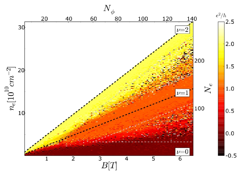
Figure 7. Hall conductivity, $\sigma_{xy}$, for the lowest two spin levels of a HF-interacting system of size $L=300$nm with disorder strength $W/d^{2}=2.5$meV in the $(B,n_{\rm e})$-plane. The two spin levels are well separated by virtue of the exchange enhancement of the spin splitting. Integer filling factors are indicated by the black broken lines, whereas the grey broken lines indicate boundaries between linear and non-linear screening [29].

We have also indicated the boundary between the non-linear and the linear screening regime by grey broken lines [29].

From our numerical results, we observe wide, stable plateaus at the integer filling factors. In contrast to a single-particle calculation [52] where the widths of the plateaus depend linearly on the magnetic field $B$, the widths of the plateaus remain constant as a function of $B$ when electron-electron interactions are taken into account. Similarly to the compressibility calculations, the estimation of the cross-over between the non-linear and linear screening appears to describe the competition between disorder and interactions well. The constant width of the plateau is in agreement with the experimental finding of Ref. [12]. The expected alignment of conductance peaks along integer filling factor is, however, absent in our calculations. Instead, we observe seemingly random conductance jumps in the centre of the bands. We attribute this behaviour to the strong exchange correlation in this regime, which was also predominant in Ref. [29], where the compressibility became strongly negative in the centre of the bands. Therefore we conclude that exchange induced effects dominate over charging and Coulomb blockade effects.

In Fig.  8 we show cross-sectional cuts in the $(B,n_{\rm e})$-plane at $B=4$T and $6$T.

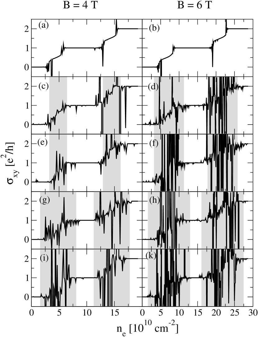
Figure 8. Hall conductivity, $\sigma_{xy}$, as cross-sectional cuts for $B=4$ (left column) and $6$ (right column) and (a,b) two spin-less Landau levels with no Coulomb interaction, (c,d) and (g,h) a spin-split Landau level at $W/d^{2}=2.5$meV and $W/d^{2}=1.25$meV, respectively. Panels (e,h) and (i,k) refer to two orbital, spin-less Landau levels at $W/d^{2}=2.5$meV and $W/d^{2}=1.25$meV, respectively. The grey areas indicate the linear screening regime [29] which widens for weaker disorder (bottom two rows).

Results for 2 Landau levels of non-interacting (a,b), strongly disordered (c,d,e,f) and weakly disordered (g,h,i,k) systems are depicted, corresponding to $2$ spin-less Landau levels (c,d,g,h) or $1$ spin-split Landau level (e,f,i,k). We have indicated the linear screening by the vertical grey shading. The plateau regions of localised electrons align well with the estimation formula of Ref. [29] and, to the accuracy of this simulation, their width is indeed independent of the magnetic field. The delocalised regime of the plateau-to-plateau transitions on the other hand increases strongly. This is in contrast to the single particle result, where both, the plateau and the transition region increases with the magnetic field. Whereas the compressibility stripes are fingerprints of the non-linear screening, i.e. the insulating regime, the increasing width of the plateau transition demonstrates an interaction promoted delocalisation. We regard this behaviour as another important manifestation of the competing interplay between disorder and electron-electron interactions even in the integer QH effect.

6. Conclusions

We have investigated numerically how the interplay of electron-electron interactions and disorder affects transport and thermodynamic properties of electrons in the IQHE. We diagonalised the Hamiltonian for electrons confined to two dimensions and subject to a perpendicular magnetic field in the suitable basis of Landau functions and treated interactions in an effective, self-consistent HF mean-field approximation. Our results are qualitatively in very good agreement with recent experiments. More quantitative statements especially regarding spin-splitting enhancement might be limited by the unscreened HF approach used in this paper. Electron correlations beyond the exchange interaction may lead to a screening of the exchange term. However, a simple replacement of the exchange term by a screened one will destroy the self-interaction cancelation occuring among Hartee and Fock term, thereby introducing a new source of error. We believe that for the purpose of this investigation our approach describes the important physical effects well [44, 53], especially for thermodynamic quantities where the system is given enough time to relax into equilibrium. The possibility to go beyond a simple electrostatic theory [54] by incorporating the exchange correlation effects, such as crystalisation and enhanced spin band separation, while at the same time allowing for the treatment of system sizes comparable to experiments, render the HF method a suitable choice. In that respect more complicated approaches such as density functional schemes [55] may not outweigh the advantages of the unscreened HF approach.

We close with some final remarks. Whereas disorder is usually associated with a reduction of signal quality, in the IQHE the concurrence of a magnetic field, reduced dimensionality, and disorder leads to a remarkable resilience of quantised transport. While the critical behaviour at the transition appears unaffected, localisation in the band tails is changed by interactions, yielding a significant change in the widths of the plateau regions. Although single-particle models can well describe many aspects of quantum Hall physics, only by taking interactions into account can the whole spectrum of experimentally observed features be satisfactorily understood.

We thankfully acknowledge discussions with J. Chalker, N. Cooper, A. Croy, N. d’Ambrumenil, K. Hashimoto, B. Huckestein, M. Morgenstern, J. Oswald, and M. Schreiber. This work has been supported partially by the Deutsche Forschungsgemeinschaft via Schwerpunktprogramm “Quantum-Hall Systeme” (Ro 1165-1/2/P).

References

- [1] K. v. Klitzing, G. Dorda, and M. Pepper, Phys. Rev. Lett. 45, 494 (1980).
- [2] R. E. Prange, Phys. Rev. B 23, 4802 (1981).
- [3] T. Chakraborty and P. Pietilänen, The Quantum Hall effects (Springer, Berlin, 1995).
- [4] M. Janssen, O. Viehweger, U. Fastenrath, and J. Hajdu, Introduction to the Theory of the Integer Quantum Hall effect (VCH, Weinheim, 1994).
- [5] R. B. Laughlin, Phys. Rev. B 23, 5632 (1981).
- [6] A. M. M. Pruisken, Nucl. Phys. B 235, 277 (1984).
- [7] D. J. Thouless, M. Kohmoto, M. P. Nightingale, and M. den Nijs, Phys. Rev. Lett. 49, 405 (1982).
- [8] A. M. M. Pruisken, in The Quantum Hall Effect, edited by R. E. Prange and S. M. Girvin (Springer, Berlin, 1987).
- [9] J. T. Chalker and P. D. Coddington, J. Phys.: Condens. Matter 21, 2665 (1988).
- [10] P. Cain and R. A. Römer, EuroPhys. Lett. 66, 104 (2004).
- [11] B. Kramer, T. Ohtsuki, and S. Kettemann, Phys. Rep. 417, 211 (2005), ArXiv: cond-mat/0409625.
- [12] D. H. Cobden, C. H. W. Barnes, and C. J. B. Ford, Phys. Rev. Lett. 82, 4695 (1999).
- [13] S. Ilani et al., Nature 427, 328 (2004).
- [14] J. Martin et al., Science 305, 980 (2004).
- [15] D. Shahar et al., Solid State Commun. 107, 19 (1998), ArXiv: cond-mat/9706045.
- [16] N. Q. Balaban, U. Meirav, and I. Bar-Jospeh, Phys. Rev. Lett. 81, 4967 (1998).
- [17] H. Aoki and T. Ando, Phys. Rev. Lett. 54, 831 (1985).
- [18] J. T. Chalker and G. J. Daniell, Phys. Rev. Lett. 61, 593 (1988).
- [19] B. Huckestein and B. Kramer, Phys. Rev. Lett. 64, 1437 (1990).
- [20] D. Liu and S. Das Sarma, Phys. Rev. B 49, 2677 (1994).
- [21] B. Huckestein, Rev. Mod. Phys. 67, 357 (1995).
- [22] J. Sinova, V. Meden, and S. M. Girvin, Phys. Rev. B 62, 2008 (2000), ArXiv: cond-mat/0002202.
- [23] P. Cain and R. A. Römer, Int. J. Mod. Phys. B 19, 2085 (2005).
- [24] A. Pruisken and I. Burmistrov, Annals of Physics 316, 285 (2005).
- [25] A. M. M. Pruisken and I. S. Burmistrov, cond-mat/0507412 (2005).
- [26] A. M. M. Pruisken and I. S. Burmistrov, cond-mat/0502488 (2005).
- [27] D.-H. Lee and Z. Wang, Phys. Rev. Lett. 76, 4014 (1996).
- [28] S.-R. E. Yang, A. H. MacDonald, and B. Huckestein, Phys. Rev. Lett. 74, 3229 (1995).
- [29] C. Sohrmann and R. A. Römer, New J. of Phys. 9, 97 (2007).
- [30] A. Pereira and J. Chalker, Physica E 31, 155 (2005), arXiv: cond-mat/0502304.
- [31] C. Sohrmann and R. A. Römer, phys. stat. sol. (b) 3, 313 (2005).
- [32] A. Struck and B. Kramer, Phys. Rev. Lett. 97, 106801 (2006).
- [33] O. E. Dial, R. C. Ashoori, L. N. Pfeiffer, and K. W. West, Nature 448, 176 (2007).
- [34] T. Ando, A. B. Fowler, and F. Stern, Rev. Mod. Phys. 54, 437 (1982).
- [35] C. Sohrmann, Ph.D. thesis, University of Warwick, 2007.
- [36] L. D. Landau and E. M. Lifshitz, Quantum Mechanics (Butterworth-Heinemann, Oxford, 1981).
- [37] C. C. J. Roothaan, Rev. Mod. Phys. 23, 69 (1951).
- [38] E. Cancès and C. L. Bris, Int. J. Quantum Chem. 79, 82 (2000).
- [39] V. R. Saunders and I. H. Hillier, Int. J. Quantum Chem. 7, 699 (1973).
- [40] R. Dombrowski et al., Phys. Rev. B 59, 8043 (1999).
- [41] M. Morgenstern et al., Phys. Rev. Lett. 89, 136806 (2002), ArXiv: cond-mat/0202239.
- [42] K. Hashimoto et al., (2007), in preparation.
- [43] A. L. Efros and B. Shklovskii, J. Phys. C 8, L49 (1975).
- [44] S.-R. Yang, Z. Wang, and A. H. MacDonald, Phys. Rev. B 65, 041302 (2001).
- [45] A. L. Efros, J. Comput. System Sci. 65, 1281 (1988).
- [46] A. L. Efros, Solid State Commun. 67, 1019 (1988).
- [47] A. L. Efros, Solid State Commun. 70, 253 (1989).
- [48] A. L. Efros, Phys. Rev. B 45, 11354 (1992).
- [49] U. Wulf, V. Gudmundsson, and R. R. Gerhardts, Phys. Rev. B 38, 4218 (1988).
- [50] J. K. Jain and S. A. Kivelson, Phys. Rev. Lett. 60, 1542 (1988).
- [51] R. Kubo, J. Phys. Soc. Japan 12, 570 (1957).
- [52] C. Sohrmann and R. A. Römer, accepted for publication in phys. stat. sol. (c) (2007).
- [53] A. H. MacDonald, H. C. A. Oji, and K. L. Liu, Phys. Rev. B 34, 2681 (1986).
- [54] D. B. Chklovskii, B. I. Shklovskii, and L. I. Glazman, Phys. Rev. B 46, 4026 (1992).
- [55] S. Ihnatsenka and I. V. Zozoulenko, Phys. Rev. B 73, 155314 (2006).