Relating Recent Infection Prevalence to Incidence with a Sub-population of Non-progressors.

Abstract

We present a new analysis of relationships between disease incidence and the prevalence of an experimentally defined state of ‘recent infection’. This leads to a clean separation between biological parameters (properties of disease progression as reflected in a test for recent infection), which need to be calibrated, and epidemiological state variables, which are estimated in a cross-sectional survey. The framework takes into account the possibility that details of the assay and host/pathogen chemistry leave a (knowable) fraction of the population in the recent category for all times. This systematically addresses an issue which is the source of some controversy about the appropriate use of the BED assay for defining recent HIV infection. Analysis of relative contributions of error arising variously from statistical considerations and simplifications of general expressions indicate that statistical error dominates heavily over all sources of bias for realistic epidemiological and biological scenarios. Numerical calculations validate the approximations made in analytical relations.

1 Introduction

Reliable estimation of disease incidence (rate of occurrence of new infections) and prevalence (the fraction of a population in an inflected state) are central to the determination of epidemiological trends, especially for the allocation of resources and evaluation of interventions. Prevalence estimation is relatively straightforward, for example by cross-sectional survey. Incidence estimates are notoriously problematic, though potentially of crucial importance. An approximate measure of incidence in a population is required for the proper planning of sample sizes and costing for clinical trials and other population based studies. Repeated follow-up of a representative cohort is often touted as the ‘gold standard’ for estimating incidence, but is costly, time intensive and still prone to some intrinsic problems. For example, there may be bias in the factors determining which subjects are lost to follow-up. Furthermore, ethical considerations demand that a cohort study involve substantial support for subjects to avoid becoming infected, which may make the cohort unrepresentative of the population of interest.

Numerous methods have been proposed for inferring incidence from single or multiple cross-sectional surveys rather than following up a cohort [1, 2, 3, 4, 5, 6, 7, 8, 9, 10]. A central idea in most of these [1, 3, 4, 5, 6, 8, 10] is to count the prevalence of a state of ‘recent infection’, which naturally depends on the recent incidence. The relationship between the two is in general not simple and depends in detail on the recent population dynamics as well as distributions which capture the inter-subject variability of progression through stages of infection, as they are observed by the specific laboratory assays used in the test for recent infection (TRI). For this approach to be sensible, a working definition of ‘recent infection’ must be calibrated, for example by repeatedly following up subjects over a period during which they become infected. This is effectively as much effort as one measurement of incidence by follow-up. The calibration is then used to infer incidence from each of many subsequent independent cross-sectional surveys.

Owing to the devastating impact of the HIV epidemic, and the many challenges of research and intervention design, the problem of estimating HIV incidence has attracted considerable interest in recent years. The prospect of using a TRI is in principle very attractive. Given the range of values of incidence likely to be observed in populations with a major epidemic (say 1-10% per annum) a mean definition of ‘recent’ of approximately half a year is desirable to yield reasonable statistical confidence for sample sizes of a few thousand. The BED assay is currently the leading candidate for such a test, but controversy has arisen about the possibility of conducting a reliable calibration. This stems from the fact that a subset of individuals (approximately $5\%$ [8, 10], potentially variable between viral and host populations) fail to progress above any statistically useful threshold set on the assay in the definition of ‘recent’ infection. This subset of individuals, who consequently remain classified as ‘recently infected’ for all times, poses a problem to which there is currently no consensus remedy.

We present a new analysis of the interaction between epidemiological trends and a model of inter-subject variability of progression through an experimental category of ‘recent infection’. Our model yields simple formulae for inference even when a fraction of the population fails to progress out of the recent category. The only physiological assumption required to deal with the non-progressors is that their survival after infection is the same as the progressors. This assumption is also implicit in previous work on using the BED assay to estimate incidence.

A key conceptual point about our analysis, which distinguishes it from all others of which we are aware, is that we confront the fundamental limitation of what can be inferred from a cross-sectional survey. In particular, even perfect knowledge of an instantaneous population state does not uniquely determine the instantaneous incidence. At best, a weighted average of recent incidence can be inferred. Although the discrepancies between this weighted average and instantaneous incidence can be shown to be small compared to statistical errors (for our application), it can in principle be systematically incorporated into estimation of trends from multiple cross-sectional surveys.

The article is organized as follows. In Section 2 we first develop a basic continuous time model defined by a time dependent incidence and susceptible population, a distribution of times after infection spent under the threshold on a TRI and a distribution of post-infection survival times. We note that there is in principle no specific relationship between the instantaneous incidence and the prevalence of individuals who are infected and under the threshold. At best, one obtains a relationship between the prevalence of under-threshold individuals and a convolution of the recent incidence with a specific weighting function which is implied by the use of a TRI. This relationship in principle includes all moments of the distribution of the waiting times that individuals spend under the threshold. We show that, for realistic rates of variation in the susceptible population, only the mean of the waiting time distribution is needed, and a simple expression for a weighted average of the incidence is obtained. The basic model is extended to allow some fraction of individuals (specified by a new parameter) to be assigned infinite waiting times under the threshold of the TRI. This leads to only very minor modifications of the previous expression for weighted incidence, namely a systematic ‘subtraction’ of over-counted ‘not recently infected’ individuals which are included in the experimental category ‘under threshold’. This subtraction is similar, but not identical, to that proposed in [10].

Section 3 explores the consequences of designing a cross-sectional survey with a sample size $N$ based on the relations derived in Section 2. Using a systematic expansion of the incidence estimator in powers of $1/\sqrt{N}$ (derived in the Appendix), we note consistency of the estimator (no bias in the limit of large $N$) and derive an approximate expression for its relative variance. These expressions facilitate error estimation both from a study design and data analysis point of view. On calibration, we note that trends, as opposed to absolute values, for incidence can be obtained without any information about the distribution of finite waiting times under the threshold. However, an estimate of the fraction of non-progressors is essential. A key observation is that, for realistic population dynamics and sample sizes, statistical error is much larger than bias.

Numerical simulations are presented in Section 4. These demonstrate that the approximate statistical analysis of Section 2 is essentially correct, with discrepancies of the size expected from the $1/\sqrt{N}$ expansion.

In the conclusion, we note that the framework presented here is quite general and is applicable to any TRI, as long as any finite probability for non-progression can be calibrated, survival is the same for progressors and non-progressors, and there is no ‘relapse’ from over to under the recency threshold. It may be possible to modify the analysis to relax these requirements. We point out that the relationship between the present analysis and other proposals for using the BED TRI for measuring HIV incidence should be more systematically investigated. Some preliminary work in this direction has already been produced [11].

2 Relating the Prevalence of ‘Recent Infection’ to Incidence

We now outline a quite general approach to relating the key demographic, epidemiological and biological processes which are relevant to the estimation of incidence from cross-sectional surveys of the prevalence of ‘recent infection’. This refines the naive intuition that a high prevalence of ‘recently infected’ individuals means a high incidence.

The Basic Model

A test for recent infection, such as the CDC STARHS algorithm, is typically obtained through the administration of two assays of different sensitivity. The more sensitive test distinguishes infected from healthy individuals and the less sensitive test, applied to the infected individuals, distinguishes ‘recent’ from ‘long’ established infection.

Consider an assay which yields a quantitative result, the value of which typically increases with time from infection. The BED assay is of this type. The quantitative result is a normalized optical density (ODn), which is an increasing function of the proportion of HIV-1 specific IgG. The hypothetical ongoing observation of an individual might lead to a curve similar to that displayed in Figure 1A. Such an assay becomes the less sensitive component of a test for recent infection when we declare a threshold value and define ‘observed to be recently infected’ to be a test value under the threshold.

In practice, there is inevitably inter-individual variation in these progression curves. Plotting the curves for multiple individuals on a single graph would lead to something like Figure 1B. Clearly, the category ‘observed to be recently infected’ is not sharply defined by a time boundary, and we now adopt the more precise labels under threshold (U) and over threshold (O). The variability of times spent in the under-threshold category, conditional on being alive long enough to reach the threshold, is captured by a distribution of waiting times $f_{\scriptscriptstyle\textrm{U}|\textrm{A}}$ which may look something like that shown in Figure 1C.

It is now possible to construct the basic epidemiological model shown in Figure 2A. Since our analysis will focus on a variety of survival functions $S(t)$, we shall refer to the susceptible population as the healthy population $H(t)$. Upon infection, individuals move from the healthy population to the under-threshold infected population $U(t)$. Those that live long enough, reach the threshold after a waiting time distributed according to $f_{\scriptscriptstyle\textrm{U}|\textrm{A}}$, and enter the over-threshold population $O(t)$. We denote by $\tau_{\scriptscriptstyle\textrm{U}|\textrm{A}}$ a waiting time generated by the density $f_{\scriptscriptstyle\textrm{U}|\textrm{A}}$. The corresponding cumulative probability function is given by

$$F_{\scriptscriptstyle\textrm{U}|\textrm{A}}(t)=\int_{0}^{t}f_{\scriptscriptstyle\textrm{U}|\textrm{A}}(s)\,ds,$$ (1)

while the probability of ‘survival’ (persistence) in the population U, conditional on being alive, is

$$S_{\scriptscriptstyle\textrm{U}|\textrm{A}}(t)=\mathbb{P}(\tau_{\scriptscriptstyle\textrm{U}|\textrm{A}}>t)=1-F_{\scriptscriptstyle\textrm{U}|\textrm{A}}(t),$$ (2)

and the mean waiting time is

$$\mathbb{E}\left[\tau_{\scriptscriptstyle\textrm{U}|\textrm{A}}\right]=\int_{0}^{\infty}\tau f_{\scriptscriptstyle\textrm{U}|\textrm{A}}(\tau)\,d\tau=\int_{0}^{\infty}S_{\scriptscriptstyle\textrm{U}|\textrm{A}}(t)\,dt.$$ (3)

Analogously, we define $f_{\scriptscriptstyle\textrm{A}}$, $\tau_{\scriptscriptstyle\textrm{A}}$, $F_{\scriptscriptstyle\textrm{A}}$, $S_{\scriptscriptstyle\textrm{A}}$ and $\mathbb{E}\left[\tau_{\scriptscriptstyle\textrm{A}}\right]$ in order to capture survival times (how long individuals remain alive after the moment of infection). We assume that survival time and waiting time to threshold are independent in this model. Hence, the probability, at a time delay $\Delta t$ after infection, of being simultaneously alive and under the threshold on the assay is

$$\mathbb{P}(\tau_{\scriptscriptstyle\textrm{A}}>\Delta t\,\,\mbox{\tiny AND}\,\,\tau_{\scriptscriptstyle\textrm{U}|\textrm{A}}>\Delta t) =S_{\scriptscriptstyle\textrm{U}}(\Delta t)=S_{\scriptscriptstyle\textrm{A}}(\Delta t)S_{\scriptscriptstyle\textrm{U}|\textrm{A}}(\Delta t).$$ (4)

Similarly, the probability of being simultaneously alive and over the threshold is

$$\mathbb{P}(\tau_{\scriptscriptstyle\textrm{A}}>\Delta t\,\,\mbox{\tiny AND}\,\,\tau_{\scriptscriptstyle\textrm{U}|\textrm{A}}\leq\Delta t) =S_{\scriptscriptstyle\textrm{A}}(\Delta t)(1-S_{\scriptscriptstyle\textrm{U}|\textrm{A}}(\Delta t)).$$ (5)

Hence, the mean time spent in the category U, accounting for both progression and mortality, is $\mathbb{E}\left[\tau_{\scriptscriptstyle\textrm{U}}\right]$.

New infections are generated by a non-homogeneous Poisson process with an intensity (probability per unit time of new arrivals) $\lambda(t)$. Let the instantaneous incidence be given by $I(t)$. Then, in a period $dt$ around time $t$, the expected number of new cases $dC$ is given by

$$dC=\lambda(t)\,dt=I(t)H(t)\,dt.$$ (6)

We can now write down numerous expressions resulting from the model. For example, the expected number of historically accumulated cases up until time $t$ is given by

$$C(t)=\int_{-\infty}^{t}\lambda(s)\,ds=\int_{-\infty}^{t}I(s)H(s)\,ds.$$ (7)

The expected populations of infected persons under and over the threshold at time $t$ are

$$U(t) =\int_{-\infty}^{t}I(s)H(s)\mathbb{P}(\tau_{\scriptscriptstyle\textrm{A}}>t-s\,\,\mbox{\tiny AND}\,\,\tau_{\scriptscriptstyle\textrm{U}|\textrm{A}}>t-s)\,ds$$

$$=\int_{-\infty}^{t}I(s)H(s)S_{\scriptscriptstyle\textrm{U}}(t-s)\,ds$$ (8)

and

$$O(t) =\int_{-\infty}^{t}I(s)H(s)\mathbb{P}(\tau_{\scriptscriptstyle\textrm{A}}>t-s\,\,\mbox{\tiny AND}\,\,\tau_{\scriptscriptstyle\textrm{U}|\textrm{A}}\leq t-s)\,ds$$

$$=\int_{-\infty}^{t}I(s)H(s)S_{\scriptscriptstyle\textrm{A}}(t-s)(1-S_{\scriptscriptstyle\textrm{U}|\textrm{A}}(t-s))\,ds.$$ (9)

Our goal is to relate $I$ for recent times to instantaneous values of $H$, $U$ and $O$. We wish to emphasize the cautionary note that there is fundamentally a loss of information when one tries to characterize the history of a population based on observations made at a single time point. The recent historical course of a population, and even instantaneous values of state variables which are rates, like incidence, are in general not inferable from counting data obtained in a single survey. This is due to the fact that counts are, unavoidably, convolutions of historical epidemiological variables, as in (8) and (9) above. Any attempt to derive incidence estimates from the counting of infections accumulated in the recent past faces this problem, and at best some sort of weighted average of the recent values of incidence can be inferred without additional assumptions.

In general, a well defined construction of an estimate for incidence, based on data obtained in a survey conducted at time $t$, will be some sort of weighted average of past values

$$I_{\scriptscriptstyle\textrm{W}}(t)=\frac{\int_{-\infty}^{t}I(s)W(s,t)\,ds}{\int_{-\infty}^{t}W(s,t)\,ds},$$ (10)

where $W(s,t)$ is a statistical weight arising from a convolution of population history and biology. Since our goal is to estimate incidence from a count of recently infected individuals, a natural weighting function is one that reflects the relative contributions to this count made by infections from different times in the recent past. Hence, we consider

$$W(s,t)=H(s)S_{\scriptscriptstyle\textrm{U}}(t-s)$$ (11)

since $W(s,t)$ is proportional to the probability that individuals are

1. available for being infected at time $s<t$, and

2. still alive and classified as under the threshold at time $t$, if infected at time $s$.

Using (11) as the weighting function leads to an expression for the incidence given by

$$I_{\scriptscriptstyle\textrm{W}}(t) =\frac{\int_{-\infty}^{t}I(s)H(s)S_{\scriptscriptstyle\textrm{U}}(t-s)\,ds}{\int_{-\infty}^{t}H(s)S_{\scriptscriptstyle\textrm{U}}(t-s)\,ds}$$

$$=\frac{U(t)}{\int_{-\infty}^{t}H(s)S_{\scriptscriptstyle\textrm{U}}(t-s)\,ds}.$$ (12)

The numerator in this expression is an instantaneous state variable, while the denominator in principle involves data from the entire history of the system as well as full knowledge of the survival function $S_{\scriptscriptstyle\textrm{U}}$.

We will shortly show how to obtain a systematic approximation of the denominator, but a few remarks are in order about the practical meaning of this weighted average. In the case of constant incidence, the weighted average is the instantaneous value. In the case of a narrowly peaked distribution $f_{\scriptscriptstyle\textrm{U}|\textrm{A}}$, a constant rate of change of $I$ and a constant healthy population, the weighted average is approximately equal to the instantaneous incidence at a time $\mathbb{E}\left[\tau_{\scriptscriptstyle\textrm{U}}\right]/2$ prior to the cross-sectional survey. If trends are fitted to the results of multiple cross-sectional surveys, this time lag could be more systematically accounted for.

A Simple Expression for Incidence

A simplified expression for weighted incidence in terms of sample and calibration data is now derived. We express the healthy population using the expansion

$$H(t+s)=H(t)+H_{1}s+H_{2}s^{2}+\ldots$$ (13)

and use the identity

$$\int_{-\infty}^{0}s^{n}S_{\scriptscriptstyle\textrm{U}}(-s)\,ds=\tfrac{(-1)^{n}}{n+1}\mathbb{E}\left[\tau_{\scriptscriptstyle\textrm{U}}^{n+1}\right],$$ (14)

which follows directly from integration by parts. It then follows that the weighted incidence (12) can be expressed as

$$I_{\scriptscriptstyle\textrm{W}}(t) =\frac{U(t)}{\int_{-\infty}^{t}H(s)S_{\scriptscriptstyle\textrm{U}}(t-s)\,ds}$$ (15)

$$=\frac{U(t)}{\int_{-\infty}^{0}H(t+s)S_{\scriptscriptstyle\textrm{U}}(-s)\,ds}$$

$$=\frac{U(t)}{H(t)\mathbb{E}\left[\tau_{\scriptscriptstyle\textrm{U}}\right]-\tfrac{H_{1}}{2}\mathbb{E}\left[\tau_{\scriptscriptstyle\textrm{U}}^{2}\right]+\ldots}.$$

If the healthy population is approximately constant for the times where the weight $W$ is non-vanishing, we obtain the simple relation

$$I_{\scriptscriptstyle\textrm{W}}=\frac{U(t)}{H(t)\,\mathbb{E}\left[\tau_{\scriptscriptstyle\textrm{U}}\right]},$$ (16)

which gives a weighted recent incidence in terms of instantaneous state variables ($H$ and $U$) and the expected waiting time in the under-threshold category.

Expectation values of the form $\mathbb{E}\left[\tau_{\scriptscriptstyle\textrm{U}}^{n}\right]$ are not state variables and should in principle be measured independently of a particular cross-sectional survey. Usually this would be accomplished in a calibration cohort follow-up study. Thus, after calibrating some of these expectation values, we can deal with a truncated expansion for $H$ without further assumptions about the behavior of $I$.

Some cautionary comments on calibration are, however, necessary. It seems unlikely that accurate measurements for terms of higher order than just $\mathbb{E}\left[\tau_{\scriptscriptstyle\textrm{U}}\right]$ are practically possible for the case of the BED assay. Finding the non-leading terms $H_{i}$ (for $i\geq 1$) in the expansion of $H$ will also require considerable demographic research.

These considerations mean that it is most likely that we will be constrained to use the simple expression (16) even if the healthy population is not approximately constant over the times where $W$ is non-vanishing. The key question then is: how severe is the bias introduced by using the simple formula under realistic non-constancy of the healthy population?

In order to explore this issue systematically we consider a non-constant healthy population given by $H(t)=H_{0}e^{\alpha t}$. This has a conveniently tunable degree of failure to conform with the constancy assumption required for (16). When $\alpha=0$ we have a constant number of healthy individuals, while a value of $\alpha=\ln(x)$ means the population grows by a factor of $x$ in one year. We can provide a survival function $S_{\scriptscriptstyle\textrm{U}}(t)$ for time measured in years, roughly inspired by the ODn progression on the BED assay, by specifying $f_{\scriptscriptstyle\textrm{U}}$ to be a Weibull distribution with scale parameter $l=0.57$ and shape parameter $k=8$. We now numerically evaluate the denominator of (15) and compare it to the denominator of the simple formula (16). Note that this bias calculation is independent of the actual time dependance in $I$.

In Figure 3, the bias in the naive denominator (reported as a fraction of the unbiased denominator) is shown as a function of $\alpha$, reported as the annual percentage growth. Note that for a population growing at $4\%$ per year, the bias is about 1.1%. As we shall see later when analyzing a slightly more complex model of a TRI, this is small compared with the statistical error that arises as a result of using realistic sample sizes. Thus, bias arising from the non-constancy of the healthy population is not a key concern unless there is very dramatic variation in $H$. The bias calculation demonstrated here is also applicable to the more complex model that now follows.

Modeling Non-progressing Individuals

A complicating factor for the BED assay is the fact that a small number of individuals utterly fail to progress beyond any practical ODn threshold used to define recency. This is due to individual variation in biochemical details such as immune response, for example. The non-progression phenomenon leads to a long term accumulation of apparently recently infected individuals, as classified by the TRI, even though many of them have been infected for a long time. There is currently no consensus on how to handle this complication. We now generalize the previous analysis to the situation where some individuals fail to progress to the over-threshold category.

Consider the simple model captured in Figure 2B. At the moment of infection, individuals transition from the healthy population to either a non-progressing population (NP) or to a progressing under-threshold population ($\textrm{P}_{\scriptscriptstyle\textrm{U}}$). The probability of non-progression is $\mathbb{P}_{{\scriptscriptstyle\textrm{NP}}}$, and hence the probability of progression is $1-\mathbb{P}_{{\scriptscriptstyle\textrm{NP}}}$. Those individuals in $\textrm{P}_{\scriptscriptstyle\textrm{U}}$ wait for a stochastic delay after which they move into the progressing over-threshold category $\textrm{P}_{\scriptscriptstyle\textrm{O}}$. In the previous model, $f_{\scriptscriptstyle\textrm{U}|\textrm{A}}$ was the distribution of waiting times governing the transition, but since the waiting times for non-progressing individuals are infinite, $f_{\scriptscriptstyle\textrm{U}|\textrm{A}}$ cannot be normalized. Therefore, in order to specify the transition times from $\textrm{P}_{\scriptscriptstyle\textrm{U}}$ to $\textrm{P}_{\scriptscriptstyle\textrm{O}}$ in terms of a normalized density, we introduce the density of waiting times in the state of being a progressor and under the threshold, conditional on being a alive, denoted by $f_{\scriptscriptstyle\textrm{PU}|\textrm{A}}$. Then $S_{\scriptscriptstyle\textrm{U}|\textrm{A}}(t)$, $S_{\scriptscriptstyle\textrm{PU}|\textrm{A}}(t)$ and $\mathbb{P}_{{\scriptscriptstyle\textrm{NP}}}$ are related by

$$S_{\scriptscriptstyle\textrm{U}|\textrm{A}}(t)=(1-\mathbb{P}_{{\scriptscriptstyle\textrm{NP}}})S_{\scriptscriptstyle\textrm{PU}|\textrm{A}}(t)+\mathbb{P}_{{\scriptscriptstyle\textrm{NP}}}.$$ (17)

The difficulty is that the TRI will classify as ‘recently infected’ all the individuals in the NP and $\textrm{P}_{\scriptscriptstyle\textrm{U}}$ categories even though some potentially large number in NP are long infected. This can systematically be addressed by the following two key steps.

Firstly, we assume that the same survival function $S_{\scriptscriptstyle\textrm{A}}$ is applicable to both progressing and non-progressing individuals. This is true if the differences between individuals which account for progression versus non-progression do not translate into significant differences in post-infection survival. This assumption has also been made, at least implicitly, in previous work on use of the BED assay for estimating HIV incidence (for example, see [11] for analysis of [8]). Its applicability should in principle be tested, but we are unaware of any evidence suggesting that it is false.

Secondly, we introduce two artificial categories by separating the non-progressing population into ‘recently infected’ (${\textrm{NP}}_{\scriptscriptstyle\textrm{R}}$) and ‘long infected’ (${\textrm{NP}}_{\scriptscriptstyle\textrm{L}}$) sub-populations. Individuals entering the ${\textrm{NP}}_{\scriptscriptstyle\textrm{R}}$ sub-population are assigned a waiting time drawn from $f_{\scriptscriptstyle\textrm{PU}|\textrm{A}}$ after which they transition to the ${\textrm{NP}}_{\scriptscriptstyle\textrm{L}}$ category. Note that this is a book-keeping device used for convenience and, unlike the assumption about survival, does not rely on any property of disease progression. It is now possible to provide a sensible definition for the class of ‘recently infected individuals’ (R) which has a population given by

$$R(t)=P_{\scriptscriptstyle\textrm{U}}(t)+{\textit{NP}}_{\scriptscriptstyle\textrm{R}}(t).$$ (18)

Note that, since both $\textrm{P}_{\scriptscriptstyle\textrm{U}}$ and ${\textrm{NP}}_{\scriptscriptstyle\textrm{R}}$ now have the same exit waiting times, the distribution of waiting times for R is given by $f_{\scriptscriptstyle\textrm{R}|\textrm{A}}=f_{\scriptscriptstyle\textrm{PU}|\textrm{A}}$, with corresponding survival function $S_{\scriptscriptstyle\textrm{R}|\textrm{A}}$.

These two steps lead to the model in Figure 2C. It is now possible to recycle our preceding analysis and write down expected counts in these new classes. Survival in the state of being simultaneously alive and recently infected, is given by $S_{\scriptscriptstyle\textrm{R}}(t)=S_{\scriptscriptstyle\textrm{A}}(t)S_{\scriptscriptstyle\textrm{R}|\textrm{A}}(t)$, and hence for the progressing populations we obtain

$$P_{\scriptscriptstyle\textrm{U}}(t) =(1-\mathbb{P}_{{\scriptscriptstyle\textrm{NP}}})\int_{-\infty}^{t}I(s)H(s)S_{\scriptscriptstyle\textrm{R}}(t-s)\,ds$$ (19)

and

$$P_{\scriptscriptstyle\textrm{O}}(t) =(1-\mathbb{P}_{{\scriptscriptstyle\textrm{NP}}})\int_{-\infty}^{t}I(s)H(s)S_{\scriptscriptstyle\textrm{A}}(t-s)(1-S_{\scriptscriptstyle\textrm{R}|\textrm{A}}(t-s))\,ds.$$ (20)

Note the similarity with expressions for $U(t)$ and $O(t)$ in the basic model. For the non-progressing populations we obtain

$${\textit{NP}}_{\scriptscriptstyle\textrm{R}}(t) =\mathbb{P}_{{\scriptscriptstyle\textrm{NP}}}\int_{-\infty}^{t}I(s)H(s)S_{\scriptscriptstyle\textrm{R}}(t-s)\,ds$$ (21)

and

$${\textit{NP}}_{\scriptscriptstyle\textrm{L}}(t) =\mathbb{P}_{{\scriptscriptstyle\textrm{NP}}}\int_{-\infty}^{t}I(s)H(s)S_{\scriptscriptstyle\textrm{A}}(t-s)(1-S_{\scriptscriptstyle\textrm{R}|\textrm{A}}(t-s))\,ds.$$ (22)

For convenience we define

$$\epsilon=\frac{\mathbb{P}_{{\scriptscriptstyle\textrm{NP}}}}{1-\mathbb{P}_{{\scriptscriptstyle\textrm{NP}}}},$$ (23)

and note that

$${\textit{NP}}_{\scriptscriptstyle\textrm{R}}(t) =\epsilon P_{\scriptscriptstyle\textrm{U}}(t)$$ (24)

and, more importantly,

$${\textit{NP}}_{\scriptscriptstyle\textrm{L}}(t) =\epsilon P_{\scriptscriptstyle\textrm{O}}(t).$$ (25)

These equations express the symmetry between the progressing and non-progressing sub-populations of Figure 2C. Substituting (19) and (21) into (18), we can write

$$R(t)=\int_{-\infty}^{t}I(s)H(s)S_{\scriptscriptstyle\textrm{R}}(t-s)\,ds.$$ (26)

It is appropriate to use a weighting scheme analogous to the one used in the basic model

$$W(s,t)=H(s)S_{\scriptscriptstyle\textrm{R}}(t-s),$$ (27)

since $W(s,t)$ is now proportional to the probability that individuals are alive and classified as recently infected at time $t$ if they become infected at time $s$, regardless of whether they are progressors or non-progressors. Then the weighted incidence, denoted $I_{\scriptscriptstyle\textrm{W}}$, is given by

$$I_{\scriptscriptstyle\textrm{W}}(t) =\frac{\int_{-\infty}^{t}I(s)H(s)S_{\scriptscriptstyle\textrm{R}}(t-s)\,ds}{\int_{-\infty}^{t}H(s)S_{\scriptscriptstyle\textrm{R}}(t-s)\,ds}$$

$$=\frac{R(t)}{\int_{-\infty}^{t}H(s)S_{\scriptscriptstyle\textrm{R}}(t-s)\,ds}.$$ (28)

The populations of under-threshold (U) and over-threshold (O) individuals are related to the populations defined in Figure 2C by

$$U(t)=P_{\scriptscriptstyle\textrm{U}}(t)+{\textit{NP}}_{\scriptscriptstyle\textrm{R}}(t)+{\textit{NP}}_{\scriptscriptstyle\textrm{L}}(t)$$ (29)

and

$$O(t)=P_{\scriptscriptstyle\textrm{O}}(t).$$ (30)

Using the above two equations and (18) and (25) this means that the population of recent infections is related to the under-threshold and over-threshold populations by

$$R(t)=U(t)-\epsilon O(t).$$ (31)

Performing the same expansion technique as before and assuming a slowly varying healthy population gives the simple expression

$$I_{\scriptscriptstyle\textrm{W}}(t)=\frac{U(t)-\epsilon O(t)}{H(t)\,\mathbb{E}\left[\tau_{\scriptscriptstyle\textrm{R}}\right]}.$$ (32)

This expresses the incidence in terms of the calibration parameters $\mathbb{E}\left[\tau_{\scriptscriptstyle\textrm{R}}\right]$ and $\epsilon$ (equivalently $\mathbb{P}_{{\scriptscriptstyle\textrm{NP}}}$), and the state variables $H$, $U$ and $O$.

All that has changed, as a result of allowing non-progressors into the model, is the shift in the numerator from $U$ to $R=U-\epsilon O$. The same bias calculations as before apply immediately, but there is an increase in statistical sensitivity. This can be understood by noting that the gross error in $U$ becomes the dominant part of a fractional error in $R$ and that $R$ is smaller than $U$.

3 Statistics and Calibration

The population models of the preceding section are expected to be in ever closer correspondence to a real population as the population size increases. To model the sampling process of a cross-sectional survey with a sample size $N$, we rescale the sub-populations of the continuous time model, at any time $t$, by the total population size $T=H+U+O$, to obtain the population proportions $\mathbb{P}_{{\scriptscriptstyle\textrm{H}}}=H/T$, $\mathbb{P}_{{\scriptscriptstyle\textrm{U}}}=U/T$ and $\mathbb{P}_{{\scriptscriptstyle\textrm{O}}}=O/T$. The result of a survey employing the TRI is the set of three counts $N_{\scriptscriptstyle\textrm{H}}+N_{\scriptscriptstyle\textrm{U}}+N_{\scriptscriptstyle\textrm{O}}=N$. These counts are trinomially distributed around their means $\bar{N}_{\scriptscriptstyle\textrm{H}}=\mathbb{P}_{{\scriptscriptstyle\textrm{H}}}N$, $\bar{N}_{\scriptscriptstyle\textrm{U}}=\mathbb{P}_{{\scriptscriptstyle\textrm{U}}}N$ and $\bar{N}_{\scriptscriptstyle\textrm{O}}=\mathbb{P}_{{\scriptscriptstyle\textrm{O}}}N$. These observed counts turn equation (32) into an estimator for the recently weighted incidence $I_{\scriptscriptstyle\textrm{est}}$ given by

$$I_{\scriptscriptstyle\textrm{est}}=\frac{1}{\mathbb{E}\left[\tau_{\scriptscriptstyle\textrm{R}}\right]}\frac{N_{\scriptscriptstyle\textrm{U}}-\epsilon N_{\scriptscriptstyle\textrm{O}}}{N_{\scriptscriptstyle\textrm{H}}}.$$ (33)

It should be noted that we do not address issues relating to experiment design and selection bias.

Statistical Fluctuations

As noted in the preceding section, in a relatively established epidemic where the smallest class is U, the major source of fluctuations in $I_{\scriptscriptstyle\textrm{est}}$ is $N_{\scriptscriptstyle\textrm{U}}$. Crudely speaking then, we can estimate the reproducibility by blaming all the statistical uncertainty on the measurement of $N_{\scriptscriptstyle\textrm{U}}$, which has a standard deviation $\sigma(N_{\scriptscriptstyle\textrm{U}})=\sqrt{N\mathbb{P}_{{\scriptscriptstyle\textrm{U}}}(1-\mathbb{P}_{{\scriptscriptstyle\textrm{U}}})}\approx\sqrt{N\mathbb{P}_{{\scriptscriptstyle\textrm{U}}}}$. This leads to the ‘back of the envelope’ formula for the relative standard deviation given by

$$\frac{\sigma(I_{\scriptscriptstyle\textrm{est}})}{I_{\scriptscriptstyle\textrm{est}}}\approx\frac{1}{\mathbb{P}_{{\scriptscriptstyle\textrm{U}}}-\epsilon\mathbb{P}_{{\scriptscriptstyle\textrm{O}}}}\sqrt{\frac{\mathbb{P}_{{\scriptscriptstyle\textrm{U}}}}{N}}.$$ (34)

However, the trinomial counts in the estimator (33) fluctuate and are correlated since they are constrained to add up to the sample size $N$. In the Appendix we demonstrate how these counts can be modeled by two independent draws ($\alpha_{1}$ and $\alpha_{2}$) from a standard normal distribution. We obtain a particular incidence estimator by inserting the counts, as functions of $\alpha_{1}$ and $\alpha_{2}$ into (33). Organizing the resulting expression into a natural expansion in powers of $1/\sqrt{N}$ gives

$$I_{\scriptscriptstyle\textrm{est}}(\alpha_{1},\alpha_{2})=I_{\scriptscriptstyle\textrm{est}}(0,0)-\frac{1}{\sqrt{N}}\left[\alpha_{1}\frac{\gamma_{1}(\mathbb{P}_{{\scriptscriptstyle\textrm{U}}}-\epsilon\mathbb{P}_{{\scriptscriptstyle\textrm{O}}})}{\mathbb{P}_{{\scriptscriptstyle\textrm{H}}}^{2}(\mathbb{P}_{{\scriptscriptstyle\textrm{O}}}+\mathbb{P}_{{\scriptscriptstyle\textrm{U}}})}+\alpha_{2}\frac{\gamma_{2}(1+\epsilon)}{\mathbb{P}_{{\scriptscriptstyle\textrm{H}}}}\right]\frac{1}{\mathbb{E}\left[\tau_{\scriptscriptstyle\textrm{R}}\right]}+O\left(\frac{1}{N}\right),$$ (35)

where

$$\gamma_{1}=\sqrt{\mathbb{P}_{{\scriptscriptstyle\textrm{H}}}(1-\mathbb{P}_{{\scriptscriptstyle\textrm{H}}})}\qquad\mbox{and}\qquad\gamma_{2}=\sqrt{\frac{\mathbb{P}_{{\scriptscriptstyle\textrm{O}}}\mathbb{P}_{{\scriptscriptstyle\textrm{U}}}}{\mathbb{P}_{{\scriptscriptstyle\textrm{O}}}+\mathbb{P}_{{\scriptscriptstyle\textrm{U}}}}}$$ (36)

The leading term,

$$I_{\scriptscriptstyle\textrm{est}}(0,0)=\frac{1}{\mathbb{E}\left[\tau_{\scriptscriptstyle\textrm{R}}\right]}\frac{\bar{N}_{\scriptscriptstyle\textrm{U}}-\epsilon\bar{N}_{\scriptscriptstyle\textrm{O}}}{\bar{N}_{\scriptscriptstyle\textrm{H}}}=\frac{1}{\mathbb{E}\left[\tau_{\scriptscriptstyle\textrm{R}}\right]}\frac{\mathbb{P}_{{\scriptscriptstyle\textrm{U}}}-\epsilon\mathbb{P}_{{\scriptscriptstyle\textrm{O}}}}{\mathbb{P}_{{\scriptscriptstyle\textrm{H}}}},$$ (37)

is just the estimator evaluated at the expectation values of the counts. The $O(1/N)$ term, which we have omitted, contains a term proportional to $\alpha_{1}^{2}$. This means that there is in principle a finite sample size bias in the estimator, which is however suppressed by $O(1/N)$ relative to the dominant term, as is borne out by numerical calculations in Section 4. The retained sub-leading term (of order $O(1/\sqrt{N})$) is distributed according to a bivariate normal distribution. Thus, to this order, there is no bias and we can read off the likelihood of observing a value of $I_{\scriptscriptstyle\textrm{est}}$,

$$L(I_{\scriptscriptstyle\textrm{est}})=f\left(\frac{I_{\scriptscriptstyle\textrm{est}}-I_{\scriptscriptstyle\textrm{est}}(0,0)}{\sigma(I_{\scriptscriptstyle\textrm{est}})}\right),$$ (38)

where $f(\cdot)$ is the standard normal density and

$$\frac{\sigma(I_{\scriptscriptstyle\textrm{est}})}{I_{\scriptscriptstyle\textrm{est}}(0,0)}=\sqrt{\frac{1}{N}\frac{1}{\mathbb{P}_{{\scriptscriptstyle\textrm{O}}}+\mathbb{P}_{{\scriptscriptstyle\textrm{U}}}}\left(\frac{1}{\mathbb{P}_{{\scriptscriptstyle\textrm{H}}}}+\frac{\mathbb{P}_{{\scriptscriptstyle\textrm{O}}}\mathbb{P}_{{\scriptscriptstyle\textrm{U}}}(1+\epsilon)^{2}}{(\mathbb{P}_{{\scriptscriptstyle\textrm{U}}}-\epsilon\mathbb{P}_{{\scriptscriptstyle\textrm{O}}})^{2}}\right)}.$$ (39)

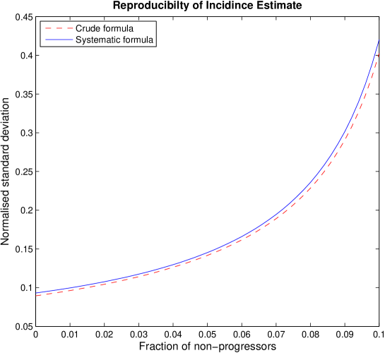
Figure 4: Plots of the crude formula (34) (dashed line) and the systematic formula (39) truncated after $O(1/\sqrt{N})$ (solid line) for the standard deviation of incidence estimates, expressed as a fraction of the leading term $I_{\scriptscriptstyle\textrm{est}}(0,0)$, and plotted as a function of the non-progressing fraction $\mathbb{P}_{{\scriptscriptstyle\textrm{NP}}}$, for fixed values $\mathbb{P}_{{\scriptscriptstyle\textrm{H}}}=0.60$, $\mathbb{P}_{{\scriptscriptstyle\textrm{U}}}=0.05$ and $\mathbb{P}_{{\scriptscriptstyle\textrm{O}}}=0.35$.

Comparison with numerical simulation suggests that this approximate result is essentially indistinguishable from the exact answer in the regime of realistic values for $N$ and the proportions ($\mathbb{P}_{{\scriptscriptstyle\textrm{H}}}$, $\mathbb{P}_{{\scriptscriptstyle\textrm{U}}}$ and $\mathbb{P}_{{\scriptscriptstyle\textrm{O}}}$), given that in practice one uses the sample proportions as estimates of the population proportions. Figure 4 plots the relations (34) and (39) for different values of $\mathbb{P}_{{\scriptscriptstyle\textrm{NP}}}$ and fixed values of $\mathbb{P}_{{\scriptscriptstyle\textrm{H}}}$, $\mathbb{P}_{{\scriptscriptstyle\textrm{O}}}$ and $\mathbb{P}_{{\scriptscriptstyle\textrm{U}}}$. Comparison with Figure 3 confirms that the truncation of the expansion of the healthy population to a constant term (the crucial step in obtaining the simple incidence relation on which the estimator is based) leads to a bias that is small compared to realistic statistical errors. The close correspondence between the two curves suggests that the simple formula (34) should be sufficiently accurate to choose a sample size for an intended study.

Calibration

Aside from the sample counts $N_{\scriptscriptstyle\textrm{H}}$, $N_{\scriptscriptstyle\textrm{U}}$ and $N_{\scriptscriptstyle\textrm{O}}$, all other quantities in relations of the kind derived in the previous section, such as $\mathbb{E}\left[\tau_{\scriptscriptstyle\textrm{R}}\right]$ in the estimator, should be regarded as parameters that need to be estimated independently of a cross-sectional survey used to infer incidence. Even in the more general case, where the healthy population is allowed to vary considerably over the time when the weighting function is non-vanishing, calibration consists only of estimating $\mathbb{P}_{{\scriptscriptstyle\textrm{NP}}}$ and expressions of the form $\mathbb{E}\left[\tau_{\scriptscriptstyle\textrm{R}}^{n}\right]$. We have already remarked that for the BED assay it will probably not be possible to obtain reasonable estimates of $\mathbb{E}\left[\tau_{\scriptscriptstyle\textrm{R}}^{n}\right]$ for values of $n$ other than $1$ and that it appears that only this term is really needed for practical purposes.

Note that if one wishes merely to estimate trends in incidence, as opposed to absolute incidence values, then it is not necessary to have an estimate for $\mathbb{E}\left[\tau_{\scriptscriptstyle\textrm{R}}\right]$ at all, since it is just an overall factor. If the overall scale of incidence estimates is to be known, considerable effort will need to be invested in the estimation of $\mathbb{E}\left[\tau_{\scriptscriptstyle\textrm{R}}\right]$. Note that this is the mean time progressing individuals spend under the threshold, with mortality accounted for.

However, surveys conducted at different times will not yield comparable values of $I_{\scriptscriptstyle\textrm{est}}\propto(U-\epsilon O)/H$ unless $\epsilon$ (equivalently $\mathbb{P}_{{\scriptscriptstyle\textrm{NP}}}$) is known with some accuracy, since it appears in one of two terms in the numerator. Consider two surveys which use the same point estimate

$$\epsilon=\epsilon_{0}+\epsilon_{1},$$ (40)

where $\epsilon_{0}$ is the real value and $\epsilon_{1}$ is the error due to methodological and statistical factors. The first survey obtains values of $N_{\scriptscriptstyle\textrm{H}}^{(1)}$, $N_{\scriptscriptstyle\textrm{U}}^{(1)}$ and $N_{\scriptscriptstyle\textrm{O}}^{(1)}$ and the second obtains values of $N_{\scriptscriptstyle\textrm{H}}^{(2)}$, $N_{\scriptscriptstyle\textrm{U}}^{(2)}$ and $N_{\scriptscriptstyle\textrm{O}}^{(2)}$. This leads to an estimate of the difference between the two incidences of

$$\Delta I_{\scriptscriptstyle\textrm{est}}(\epsilon)=I_{\scriptscriptstyle\textrm{est}}^{(1)}(\epsilon)-I_{\scriptscriptstyle\textrm{est}}^{(2)}(\epsilon)=\frac{N_{\scriptscriptstyle\textrm{U}}^{(1)}-\epsilon N_{\scriptscriptstyle\textrm{O}}^{(1)}}{N_{\scriptscriptstyle\textrm{H}}^{(1)}\mathbb{E}\left[\tau_{\scriptscriptstyle\textrm{R}}\right]}-\frac{N_{\scriptscriptstyle\textrm{U}}^{(2)}-\epsilon N_{\scriptscriptstyle\textrm{O}}^{(2)}}{N_{\scriptscriptstyle\textrm{H}}^{(2)}\mathbb{E}\left[\tau_{\scriptscriptstyle\textrm{R}}\right]}.$$ (41)

Knowledge of the exact value $\epsilon_{0}$ leads to

$$\Delta I_{\scriptscriptstyle\textrm{est}}(\epsilon_{0})=I_{\scriptscriptstyle\textrm{est}}^{(1)}(\epsilon_{0})-I_{\scriptscriptstyle\textrm{est}}^{(2)}(\epsilon_{0})=\frac{N_{\scriptscriptstyle\textrm{U}}^{(1)}-\epsilon_{0}N_{\scriptscriptstyle\textrm{O}}^{(1)}}{N_{\scriptscriptstyle\textrm{H}}^{(1)}\mathbb{E}\left[\tau_{\scriptscriptstyle\textrm{R}}\right]}-\frac{N_{\scriptscriptstyle\textrm{U}}^{(2)}-\epsilon_{0}N_{\scriptscriptstyle\textrm{O}}^{(2)}}{N_{\scriptscriptstyle\textrm{H}}^{(2)}\mathbb{E}\left[\tau_{\scriptscriptstyle\textrm{R}}\right]},$$ (42)

from which we see that the error in $\Delta I_{\scriptscriptstyle\textrm{est}}$, due to the error in $\epsilon$, is

$$\Delta I_{\scriptscriptstyle\textrm{est}}(\epsilon)-\Delta I_{\scriptscriptstyle\textrm{est}}(\epsilon_{0})=\frac{\epsilon_{1}}{\mathbb{E}\left[\tau_{\scriptscriptstyle\textrm{R}}\right]}\left(\frac{N_{\scriptscriptstyle\textrm{O}}^{(2)}}{N_{\scriptscriptstyle\textrm{H}}^{(2)}}-\frac{N_{\scriptscriptstyle\textrm{O}}^{(1)}}{N_{\scriptscriptstyle\textrm{H}}^{(1)}}\right).$$ (43)

The direction and magnitude of error depend in detail on many factors, such as population renewal and long term post-infection survival. While it is not possible to summarize all the effects that may be produced by imperfect estimation of $\mathbb{P}_{{\scriptscriptstyle\textrm{NP}}}$, in Section 4 we conduct a number of numerical simulations which demonstrate the kind of bias that may arise.

4 Numerical Simulations

In this section we briefly outline two numerical simulations. The first serves to test the accuracy of the bias and standard deviation estimates derived from the truncation of the systematic expansion of the stochastic estimator $I_{\scriptscriptstyle\textrm{est}}(\alpha_{1},\alpha_{2})$. For each of 10,000,000 iterations, two standard normal variables were drawn. Counts for healthy, under-threshold and over-threshold sub-populations, within a sample of size $N=5000$, were generated according to the procedure provided in the Appendix. This algorithm incorporates the assumption that the trinomial distribution of the sample proportions can be approximated as normal, but involves no truncation of the estimator in powers of $1/\sqrt{N}$. The resulting ensemble of point estimates $I_{\scriptscriptstyle\textrm{est}}$ produced suitably converged estimates for the mean and standard deviation.

The entire procedure of the preceding paragraph was repeated for values of $\mathbb{P}_{{\scriptscriptstyle\textrm{O}}}\in[0.1,0.5]$. For each value of $\mathbb{P}_{{\scriptscriptstyle\textrm{O}}}$, the value of $\mathbb{P}_{{\scriptscriptstyle\textrm{U}}}$ was varied to produce an incidence in the range $[0.01,0.2]$. The average fractional discrepancy between the mean incidence and $I_{\scriptscriptstyle\textrm{est}}(0,0)$ was 0.0003, with values ranging from 0.00001 to 0.0008, confirming that the intrinsic sampling bias is of order $1/N$. The average fractional discrepancy between the observed standard deviation of the incidence and the approximate expression (39) was 0.0006, with values ranging from 0.00004 to 0.001, which is also consistent with the truncation at $O(1/\sqrt{N})$.

A second simulation demonstrates the use of the simple expression (33) for incidence estimation. Arrival times of new infections were generated according to a non-homogeneous Poisson process with intensity given by $\lambda(t)=H(t)I(t)$ as described in more detail below. Newly infected individuals were initially classified as under the recency threshold of a TRI. A fraction $1-\mathbb{P}_{{\scriptscriptstyle\textrm{NP}}}$ progressed to the over-threshold category according to waiting times generated by $f_{\scriptscriptstyle\textrm{R}|\textrm{A}}$. Weibull functions were used for the waiting time distributions $f_{\scriptscriptstyle\textrm{R}|\textrm{A}}$ and $f_{\scriptscriptstyle\textrm{A}}$. Unique individuals were drawn from the population at intervals, to produce counts $N_{\scriptscriptstyle\textrm{H}}$, $N_{\scriptscriptstyle\textrm{U}}$ and $N_{\scriptscriptstyle\textrm{O}}$, and hence estimates for incidence.

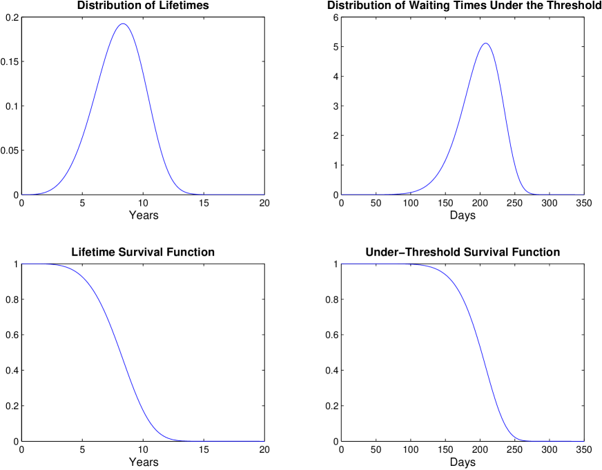
Figure 5: Graphical representation of the densities $f_{\scriptscriptstyle\textrm{A}}$ and $f_{\scriptscriptstyle\textrm{R}|\textrm{A}}$ for survival times and times under threshold in the progressing population (top) and the corresponding survival probabilities $S_{\scriptscriptstyle\textrm{A}}$ and $S_{\scriptscriptstyle\textrm{R}|\textrm{A}}$ (bottom). Parameters for these curves are detailed in Table 1.

To demonstrate the incidence estimation process, a $50$ year population scenario was produced. Figure 5 shows the Weibull distributions used for $f_{\scriptscriptstyle\textrm{A}}$ and $f_{\scriptscriptstyle\textrm{R}|\textrm{A}}$ (top) and the corresponding survival curves $S_{\scriptscriptstyle\textrm{A}}$ and $S_{\scriptscriptstyle\textrm{R}|\textrm{A}}$ (bottom). The Weibull shape and scale parameters for the distributions were chosen to give approximately realistic values for the mean and standard deviations for the window period and infected life expectancy, as detailed in Table 1. The healthy population was set to $H(t)=100,000+5,000t$, with $t$ measured in years. The incidence was set at $0.01$ (hazard per person per year) for the first ten years, climbing linearly to 0.1 over the next ten years, then remaining at this high level for a further ten years, followed by ten years of linear decline to $0.03$ and maintained at this level for the last ten years of the simulation.

	Shape ($k$)	Scale ($l$)	Mean	Standard Dev.
Life expectancy ($f_{\scriptscriptstyle\textrm{A}}$)	4.5	8.83	8 years	2 years
Window period ($f_{\scriptscriptstyle\textrm{R}|\textrm{A}}$)	8	0.58	200 days	30 days

Table 1: Weibull parameters for the Monte Carlo simulation (survival time measured in years).

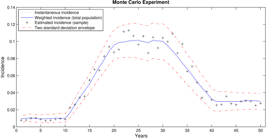
Figure 6: Full stochastic simulation of population with epidemic, individual survival times, and annual sampling of $5,000$ individuals. The healthy population was set to $H(t)=100,000+5,000t$ with time measured in years. The instantaneous incidence parameter is the dotted curve. The target of the estimates is the weighted incidence (solid line), which was calculated explicitly as per (28) from all the known inputs. This is flanked by a two standard deviation envelope (dashed lines). Simulated estimated incidence ($+$ symbols) were obtained by using sample counts in the simple estimator (33). The calibration parameters $\mathbb{E}\left[\tau_{\scriptscriptstyle\textrm{R}}\right]$ and $\mathbb{P}_{{\scriptscriptstyle\textrm{NP}}}$ were assumed to be known exactly.

Figure 6 shows output from this simulation. The input incidence parameter is indicated as the dotted instantaneous incidence curve. A sample of $5,000$ individuals was surveyed every year, and an incidence estimate was produced using the simple estimator (33) with exact values of $\mathbb{E}\left[\tau_{\scriptscriptstyle\textrm{R}}\right]$ and $\mathbb{P}_{{\scriptscriptstyle\textrm{NP}}}$, i.e., assuming perfect calibration. These point estimates are indicated as estimated incidence values, using ‘$+$’ symbols. The combined effects of the previously noted time convolution, in $I_{\scriptscriptstyle\textrm{W}}$, as well as stochastic departure from means in the simulated population, make the input incidence parameter an unrealistic target for simulated incidence measurements. Thus, the solid weighted incidence line has been displayed, which uses full knowledge of all population members’ classification into H, U or O, inserted into (28) with full knowledge of the denominator, (both the non-constant $H(t)$ and the exact $S_{\scriptscriptstyle\textrm{R}}$). This is essentially all that the incidence estimation algorithm can be asked to reproduce. A two standard deviation envelope around the weighted incidence line, calculated from (39) using knowledge of the full population, is shown as two dashed lines.

In Section 3 it was shown that incidence trends can be extracted without $\mathbb{E}\left[\tau_{\scriptscriptstyle\textrm{R}}\right]$ calibration, while an estimate for $\mathbb{P}_{{\scriptscriptstyle\textrm{NP}}}$ is vital. We now explore the extent to which the accuracy of the estimate of $\mathbb{P}_{{\scriptscriptstyle\textrm{NP}}}$ affects the ability to determine a trend in incidence.

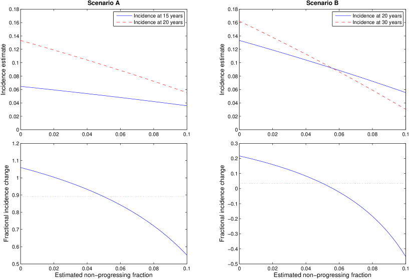
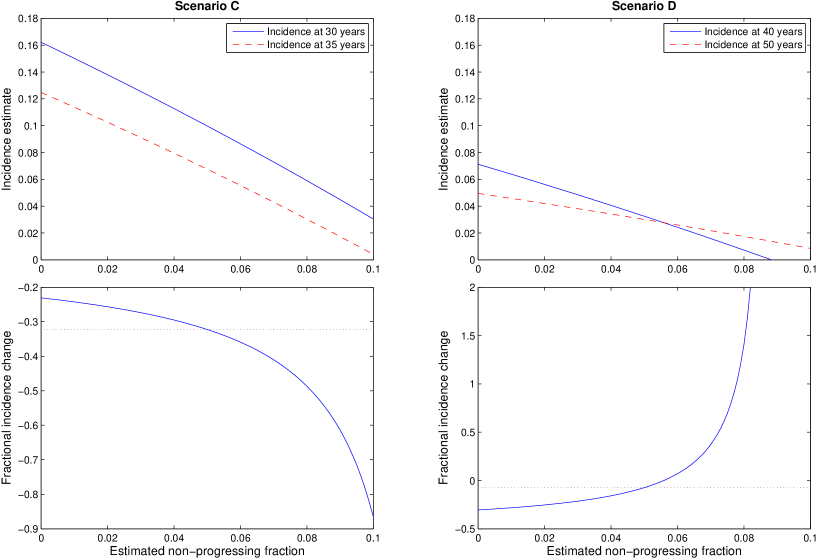
Figure 7: Absolute incidence estimates and estimated fractional incidence changes for four pairs of successive times from Table 2.

Population fractions for H, U and O were extracted at six times from the population simulation described above and are shown in Table 2. Four instances of incidence trend estimation were simulated by selecting the time intervals $(15,20)$, $(20,30)$, $(30,35)$ and $(40,50)$. We considered the trends that would be observed if incidence were measured at the beginning and end of each of these intervals using (37). In order to focus on the bias introduced by imperfect estimation of $\mathbb{P}_{{\scriptscriptstyle\textrm{NP}}}$, rather than sample size effects, we assumed perfect knowledge of $\mathbb{P}_{{\scriptscriptstyle\textrm{H}}}$, $\mathbb{P}_{{\scriptscriptstyle\textrm{U}}}$ and $\mathbb{P}_{{\scriptscriptstyle\textrm{O}}}$. For each of these intervals, we calculated an incidence estimate at the beginning and end, as a function of the estimated value of $\mathbb{P}_{{\scriptscriptstyle\textrm{NP}}}$ (the true value being $0.05$), assuming $\mathbb{E}\left[\tau_{\scriptscriptstyle\textrm{R}}\right]$ is known exactly. We also calculated the estimated fractional change in incidence over each interval. Note that the fractional change does not depend on $\mathbb{E}\left[\tau_{\scriptscriptstyle\textrm{R}}\right]$. The results are shown in Figure 7, where the four intervals $(15,20)$, $(20,30)$, $(30,35)$ and $(40,50)$ are referred to as scenarios A, B, C and D, respectively.

In each case, the effect of the error in the estimation of $\mathbb{P}_{{\scriptscriptstyle\textrm{NP}}}$ is quite different, as can be understood by considering how (43) is impacted by the system history. Note that case B and case D both simulate intervals over which incidence is approximately constant, but the impact (on the estimated incidence change) of incorrect estimation of $\mathbb{P}_{{\scriptscriptstyle\textrm{NP}}}$ does not even agree in sign. At a time of $40$ years, the incidence estimate becomes negative when the $\mathbb{P}_{{\scriptscriptstyle\textrm{NP}}}$ estimate is higher than $0.0882$. This breakdown of the model results in the divergence of the fractional change in estimated incidence over the interval in scenario D. In short, incorrect estimates of $\mathbb{P}_{{\scriptscriptstyle\textrm{NP}}}$ can lead to the fundamental breakdown of the inference scheme. This makes sense, as $\mathbb{P}_{{\scriptscriptstyle\textrm{NP}}}$ impacts the long term accumulation of individuals in the $\mathbb{P}_{{\scriptscriptstyle\textrm{O}}}$ category.

	Time (years)
	15	20	30	35	40	50
$\mathbb{P}_{{\scriptscriptstyle\textrm{H}}}$	0.849	0.687	0.576	0.602	0.694	0.814
$\mathbb{P}_{{\scriptscriptstyle\textrm{U}}}$	0.030	0.050	0.051	0.041	0.027	0.022
$\mathbb{P}_{{\scriptscriptstyle\textrm{O}}}$	0.121	0.263	0.373	0.357	0.279	0.164

Table 2: Population fractions in H, U and O within a 50 year epidemic scenario.

5 Discussion and Conclusion

We have presented a detailed analysis of relations between recent incidence in a population and counts of ‘recently infected’ individuals. These are in principle complex convolutions involving the epidemiological history as well as all information about the distribution of waiting times in the recently infected category. When the healthy population undergoes realistically modest variation on the time scale of the definition of recency implied by the TRI, we obtain simplified forms which incur very little error. The simplified relations form the basis of estimators which are shown to have considerably more variance than bias under realistic demographic and epidemiological assumptions.

Noting that the assumptions of our model are the least restrictive of any BED based HIV incidence estimation method of which we are aware, we now consider its limitations. We have only modeled one direction of progression of individuals from an experimentally defined state of ‘recent’ infection to ‘non-recent’ infection. The reverse apparently occurs for BED optical density in some terminal stage AIDS patients. This process constitutes a substantial complication, and further work is required to investigate how it may be incorporated into an analytical model of the kind developed here. It may be worth exploring previous suggestions [8] to use additional information, from questionnaires or other assays, to remove end-stage patients from the observed recent count. We have also not considered the possibility that calibration parameters are functions of time, for example as a result of substantial vaccine uptake in a population. Even more subtle is a point raised under calibration, namely that imperfect estimation of the non-progressing fraction of the population leads to a complex bias in incidence estimates. This bias is dependent on factors not even present in the incidence estimator, such as long term survival post infection.

A key observation is that, for the purposes of estimating incidence from a TRI, there is no fundamental obstacle posed by having a known fraction of individuals fail to progress over the recency threshold, as long as their distribution of survival times from infection is the same as in the progressing population. In fact, an accurate estimate of this non-progressing fraction alone, is sufficient (and necessary) to infer trends in incidence. This fraction could possibly be estimated for the BED assay from historical records, since there are many viable samples in storage with supporting clinical information indicating long-infected status. However, as demonstrated in the calculations of Section 4, a suitably large error in the estimate of $\mathbb{P}_{{\scriptscriptstyle\textrm{NP}}}$ can render TRI based incidence estimates meaningless. A calibration of the mean finite waiting time is required in order to estimate absolute values of incidence. Prospective follow-up is probably the only practical way to estimate this parameter.

In contrast to our model, which has only two calibration parameters, the model of McDougal et al. [8] appears to have three (sensitivity, short-term specificity and long-term specificity). In a separate short note [11] we demonstrate that, under their own assumptions, these parameters can be reduced to ours. This has two advantages—our parameters are easier to calibrate and assuming independence of their parameters would lead to incorrect error estimates.

Besides the explicit assumptions noted, the analysis presented here is quite general. Tests for recent infection continue to be of interest, and new assays are likely to be developed both for HIV infection and other important diseases. In summary, we have presented a simple incidence estimator and a detailed analysis of its likelihood function, which can inform design of appropriate calibration studies and cross-sectional incidence estimation surveys, and can also form the basis of systematic inference algorithms for processing the data obtained from such surveys.

Appendix

Given a sample of $N$ subjects tested using the TRI, we derive a systematic expansion, in powers of $O(1/\sqrt{N})$, for the estimator

$$I_{\scriptscriptstyle\textrm{est}}=\frac{1}{\mathbb{E}\left[\tau_{\scriptscriptstyle\textrm{R}}\right]}\frac{N_{\scriptscriptstyle\textrm{U}}-\epsilon N_{\scriptscriptstyle\textrm{O}}}{N_{\scriptscriptstyle\textrm{H}}}=\frac{1}{\mathbb{E}\left[\tau_{\scriptscriptstyle\textrm{R}}\right]}\frac{P_{{\scriptscriptstyle\textrm{U}}}-\epsilon P_{{\scriptscriptstyle\textrm{O}}}}{P_{{\scriptscriptstyle\textrm{H}}}},$$ (44)

where the counts $N_{\scriptscriptstyle\textrm{X}}=P_{{\scriptscriptstyle\textrm{X}}}N$ fluctuate trinomially around their means $\bar{N_{\scriptscriptstyle\textrm{X}}}=\mathbb{P}_{{\scriptscriptstyle\textrm{X}}}N$, with standard deviations $\sigma_{\scriptscriptstyle\textrm{X}}=\sqrt{N\mathbb{P}_{{\scriptscriptstyle\textrm{X}}}(1-\mathbb{P}_{{\scriptscriptstyle\textrm{X}}})}$, or, alternatively, the realized sample proportions $P_{{\scriptscriptstyle\textrm{X}}}$ fluctuate multinomially around their means $\mathbb{P}_{{\scriptscriptstyle\textrm{X}}}$, with standard deviations $\sigma_{P_{{\scriptscriptstyle\textrm{X}}}}=\sqrt{\mathbb{P}_{{\scriptscriptstyle\textrm{X}}}(1-\mathbb{P}_{{\scriptscriptstyle\textrm{X}}})/N}$. In order to account for fluctuations in the sample counts, as well as their correlations, we express the three counts as the result of two independent random draws. We assume the counts are sufficiently large so that binomial distributions can be approximated by normal distributions—which will be the case if the survey is to have any reasonable accuracy.

• Draw a number $\alpha_{1}$ from a standard normal distribution and set

  $$N_{\scriptscriptstyle\textrm{H}}=\bar{N}_{\scriptscriptstyle\textrm{H}}+\sigma_{1}\alpha_{1},$$ (45)

  where

  $$\sigma_{1}=\sigma_{\scriptscriptstyle\textrm{S}}=\sqrt{N\mathbb{P}_{{\scriptscriptstyle\textrm{H}}}(1-\mathbb{P}_{{\scriptscriptstyle\textrm{H}}})}=\sqrt{N}\gamma_{1}.$$ (46)

  Defining $\gamma_{1}$ allows us to keep track of powers of $1/\sqrt{N}$.

• Draw a number $\alpha_{2}$ from a standard normal distribution and set

  $$N_{\scriptscriptstyle\textrm{U}} =\mathbb{P}_{{\scriptscriptstyle\textrm{U}}}^{\prime}(N-N_{\scriptscriptstyle\textrm{H}})+\sigma_{2}\alpha_{2}$$

  $$=\mathbb{P}_{{\scriptscriptstyle\textrm{U}}}^{\prime}N(1-\mathbb{P}_{{\scriptscriptstyle\textrm{H}}})-\mathbb{P}_{{\scriptscriptstyle\textrm{U}}}^{\prime}\sigma_{1}\alpha_{1}+\sigma_{2}\alpha_{2}$$

  $$=\mathbb{P}_{{\scriptscriptstyle\textrm{U}}}N-\mathbb{P}_{{\scriptscriptstyle\textrm{U}}}^{\prime}\gamma_{1}\alpha_{1}\sqrt{N}+\sigma_{2}\alpha_{2}$$ (47)

  and

  $$N_{\scriptscriptstyle\textrm{O}} =\mathbb{P}_{{\scriptscriptstyle\textrm{O}}}^{\prime}(N-N_{\scriptscriptstyle\textrm{H}})-\sigma_{2}\alpha_{2}$$

  $$=\mathbb{P}_{{\scriptscriptstyle\textrm{O}}}^{\prime}N(1-\mathbb{P}_{{\scriptscriptstyle\textrm{H}}})-\mathbb{P}_{{\scriptscriptstyle\textrm{O}}}^{\prime}\sigma_{1}\alpha_{1}-\sigma_{2}\alpha_{2}$$

  $$=\mathbb{P}_{{\scriptscriptstyle\textrm{O}}}N-\mathbb{P}_{{\scriptscriptstyle\textrm{O}}}^{\prime}\gamma_{1}\alpha_{1}\sqrt{N}-\sigma_{2}\alpha_{2}$$ (48)

  where

  $$\mathbb{P}_{{\scriptscriptstyle\textrm{U}}}^{\prime}=\frac{\mathbb{P}_{{\scriptscriptstyle\textrm{U}}}}{\mathbb{P}_{{\scriptscriptstyle\textrm{U}}}+\mathbb{P}_{{\scriptscriptstyle\textrm{O}}}}\qquad\mbox{and}\qquad\mathbb{P}_{{\scriptscriptstyle\textrm{O}}}^{\prime}=1-\mathbb{P}_{{\scriptscriptstyle\textrm{U}}}^{\prime}$$ (49)

  are the probabilities of an individual being in U and O given that they are not in H, and

  $$\sigma_{2}=\sigma_{{\scriptscriptstyle\textrm{B}}|\alpha_{1}}=\sqrt{(N-N_{\scriptscriptstyle\textrm{H}})\mathbb{P}_{{\scriptscriptstyle\textrm{U}}}^{\prime}\mathbb{P}_{{\scriptscriptstyle\textrm{O}}}^{\prime}}=\sqrt{N}\gamma_{2}\left(1+O\left(\tfrac{1}{\sqrt{N}}\right)\right)$$ (50)

  is the standard deviation of $N_{\scriptscriptstyle\textrm{U}}$ (and $N_{\scriptscriptstyle\textrm{O}}$) subject to $\alpha_{1}$ having been determined, so that

  $$\gamma_{2}=\sqrt{\frac{\mathbb{P}_{{\scriptscriptstyle\textrm{O}}}\mathbb{P}_{{\scriptscriptstyle\textrm{U}}}}{\mathbb{P}_{{\scriptscriptstyle\textrm{O}}}+\mathbb{P}_{{\scriptscriptstyle\textrm{U}}}}}.$$ (51)

The sample proportions can now be written as:

$$P_{{\scriptscriptstyle\textrm{H}}} =\mathbb{P}_{{\scriptscriptstyle\textrm{H}}}+\tfrac{1}{\sqrt{N}}\alpha_{1}\gamma_{1}$$

$$P_{{\scriptscriptstyle\textrm{U}}} =\mathbb{P}_{{\scriptscriptstyle\textrm{U}}}-\tfrac{1}{\sqrt{N}}\big{(}\alpha_{1}\mathbb{P}_{{\scriptscriptstyle\textrm{U}}}^{\prime}\gamma_{1}-\alpha_{2}\gamma_{2}\big{)}+O\left(\tfrac{1}{N}\right)$$

$$P_{{\scriptscriptstyle\textrm{O}}} =\mathbb{P}_{{\scriptscriptstyle\textrm{O}}}-\tfrac{1}{\sqrt{N}}\big{(}\alpha_{1}\mathbb{P}_{{\scriptscriptstyle\textrm{O}}}^{\prime}\gamma_{1}+\alpha_{2}\gamma_{2}\big{)}+O\left(\tfrac{1}{N}\right)$$ (52)

Note that this procedure works independently of the order in which the values of $N_{\scriptscriptstyle\textrm{H}}$, $N_{\scriptscriptstyle\textrm{U}}$ and $N_{\scriptscriptstyle\textrm{O}}$ are assigned from the random $\alpha$’s. We can explicitly insert this decomposition into the expression for $I_{\scriptscriptstyle\textrm{est}}$ to obtain an expression for the estimator in terms of two independent draws from a standard normal distribution. Keeping only the $O(1)$ and $O(1/\sqrt{N})$ terms explicit leads to

$$I_{\scriptscriptstyle\textrm{est}}(\alpha_{1},\alpha_{2})=I_{\scriptscriptstyle\textrm{est}}(0,0)-\frac{1}{\sqrt{N}}\left[\alpha_{1}\frac{\gamma_{1}(\mathbb{P}_{{\scriptscriptstyle\textrm{U}}}-\epsilon\mathbb{P}_{{\scriptscriptstyle\textrm{O}}})}{\mathbb{P}_{{\scriptscriptstyle\textrm{H}}}^{2}(\mathbb{P}_{{\scriptscriptstyle\textrm{O}}}+\mathbb{P}_{{\scriptscriptstyle\textrm{U}}})}+\alpha_{2}\frac{\gamma_{2}(1+\epsilon)}{\mathbb{P}_{{\scriptscriptstyle\textrm{H}}}}\right]\frac{1}{\mathbb{E}\left[\tau_{\scriptscriptstyle\textrm{R}}\right]}+O\left(\frac{1}{N}\right),$$ (53)

where

$$I_{\scriptscriptstyle\textrm{est}}(0,0)=\frac{1}{\mathbb{E}\left[\tau_{\scriptscriptstyle\textrm{R}}\right]}\frac{\mathbb{P}_{{\scriptscriptstyle\textrm{U}}}-\epsilon\mathbb{P}_{{\scriptscriptstyle\textrm{O}}}}{\mathbb{P}_{{\scriptscriptstyle\textrm{H}}}}.$$ (54)

Two key observations immediately follow:

• The proposed $I_{\scriptscriptstyle\textrm{est}}$ is a consistent estimator in the sense that terms with bias are at least $O(1/N)$ suppressed relative to the dominant term.

• To order $O(1/\sqrt{N})$, $I_{\scriptscriptstyle\textrm{est}}$ is Gaussian with relative variance

  $$\left(\frac{\sigma(I_{\scriptscriptstyle\textrm{est}})}{I_{\scriptscriptstyle\textrm{est}}(0,0)}\right)^{2}=\frac{1}{N}\frac{1}{\mathbb{P}_{{\scriptscriptstyle\textrm{O}}}+\mathbb{P}_{{\scriptscriptstyle\textrm{U}}}}\left(\frac{1}{\mathbb{P}_{{\scriptscriptstyle\textrm{H}}}}+\frac{\mathbb{P}_{{\scriptscriptstyle\textrm{O}}}\mathbb{P}_{{\scriptscriptstyle\textrm{U}}}(1+\epsilon)^{2}}{(\mathbb{P}_{{\scriptscriptstyle\textrm{U}}}-\epsilon\mathbb{P}_{{\scriptscriptstyle\textrm{O}}})^{2}}\right).$$ (55)

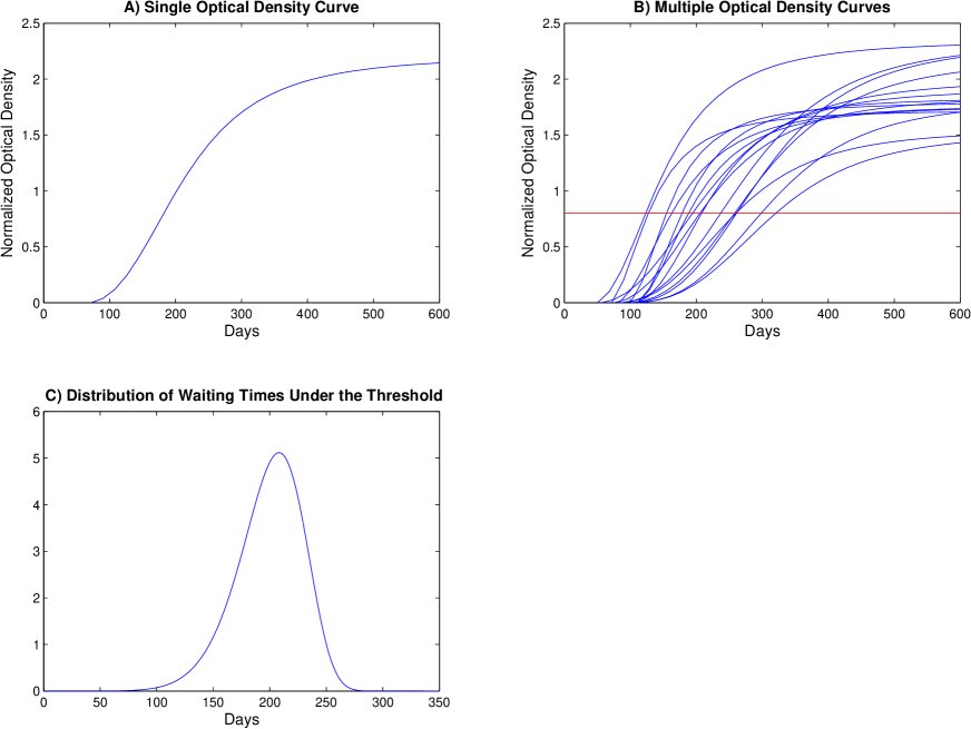
Figure 1:

1. Hypothetical individual BED normalized optical density (ODn) as a function of time since infection.

2. Hypothetical collection of individual ODn progression plots with inter-individual variability and an arbitrary ODn threshold which can be used to define recent infection.

3. Hypothetical distribution of times spent under the ODn threshold after infection, which approximately captures the mean and variance of the sample of individual progression curves in B).

Figure 2:

1. The basic epidemiological/TRI progression model. Members of the healthy population H are subject to a per unit time hazard (incidence) $I$ of infection. After infection, individuals enter the under-threshold population U. Here they spend a time distributed according to $f_{\scriptscriptstyle\textrm{U}|\textrm{A}}$, after which they spend the remainder of their lifetime, if any, in the over-threshold population O.

2. The basic model modified to accommodate non-progressors on the TRI. Now, upon infection, a proportion $\mathbb{P}_{{\scriptscriptstyle\textrm{NP}}}$ of individuals remain forever under the threshold of the TRI, i.e., they enter the NP category. The remaining proportion, $1-\mathbb{P}_{{\scriptscriptstyle\textrm{NP}}}$, the progressors, are assigned a waiting time from $f_{\scriptscriptstyle\textrm{PU}|\textrm{A}}$, and spend this time in the ‘progressing, under-threshold’ population $\textrm{P}_{\scriptscriptstyle\textrm{U}}$. Those that survive long enough spend the remainder of their lifetime in the ‘progressing, over-threshold’ population $\textrm{P}_{\scriptscriptstyle\textrm{O}}$

3. Modified model with separation of non-progressors into ‘recent’ and ‘long’ infected categories. This model contains the same epidemiology and biology as the model in B), with the introduction of a bookkeeping device which facilitates the definition of a calibratable category of ‘recently infected’ individuals. The non-progressors are assigned waiting times drawn from the distribution observed in the progressing population, and spend this waiting time in the ‘non-progressing recently infected’ (${\textrm{NP}}_{\scriptscriptstyle\textrm{R}}$) category, before moving to the ‘non-progressing long infected’ (${\textrm{NP}}_{\scriptscriptstyle\textrm{L}}$) category.

Figure 3: Fractional error in the simple incidence relation (16) versus the full relation (15), as a function of growth rate of the healthy population, quoted as a percentage annual growth. The scenario is defined by: $S(t)=S(0)e^{\alpha t}$ and $f_{\scriptscriptstyle\textrm{U}}$ is a Weibull distribution with scale parameter $l=0.57$ and shape parameter $k=8$. The parameter $\alpha$ is varied to produce deviation from a constant healthy population ($\alpha=0$) in which limit equation (16) is exact.