A Dynamical Quantum Cluster Approach to Two-Particle Correlation
Functions in the Hubbard Model

Abstract

We investigate the charge- and spin dynamical structure factors for the 2D one-band Hubbard model in the strong coupling regime within an extension of the Dynamical Cluster Approximation (DCA) to two-particle response functions. The full irreducible two-particle vertex with three momenta and frequencies is approximated by an effective vertex dependent on the momentum and frequency of the spin/charge excitation. In the spirit of the DCA, the effective vertex is calculated with quantum Monte Carlo methods on a finite cluster. On the basis of a comparison with high temperature auxiliary field quantum Monte Carlo data we show that near and beyond optimal doping, our results provide a consistent overall picture of the interplay between charge, spin and single-particle excitations.

I Introduction

Two-particle correlation functions, such as the dynamical spin- and charge correlation functions, determine a variety of crucial properties of many-body systems. Their poles as a function of frequency and momentum describe the elementary excitations, i.e. electron-hole excitations and collective modes, such as spin- and charge-density waves. Furthermore, an effective way to identify continuous phase transitions is to search for divergencies of susceptibilities, i.e. two-particle correlation functions. Yet, compared to studies of single-particle Green’s functions and their spectral properties, where a good overall accord between theoretical models (Hubbard type-models) and experiment (ARPES) has been established (see Refs. DHS2003, ; preuss95, ; preuss97, ; IFT98, ), the situation is usually not so satisfying for two-particle Green’s functions. This is especially so for the case of correlated electron systems such as high-$T_{c}$ superconductors (HTSC). The primary reason for this is that calculations of these Green’s functions are, from a numerical point of view, much more involved.

To expose the problem let us consider the spin-susceptibility which is given by:

$$\chi(\underline{q})=\frac{1}{\beta L}\sum_{\underline{k},\underline{p}}\chi_{\underline{k},\underline{p}}(\underline{q})\;\;{\rm,with}$$ (1)

$$\chi_{\underline{k},\underline{p}}(\underline{q})=\langle c^{\dagger}_{\underline{k},\uparrow}c^{\phantom{\dagger}}_{\underline{k}+\underline{q},\downarrow}c^{\dagger}_{\underline{p},\downarrow}c^{\phantom{\dagger}}_{\underline{p}-\underline{q},\uparrow}\rangle$$

Here, $L$ corresponds to the lattice size, $\beta$ is the inverse temperature and $\underline{q}\equiv({\bm{q}},\Omega_{m})$, ${\bm{q}}$ being the momentum and $\Omega_{m}$ a (bosonic) Matsubara frequency. To simplify the notation, we have adopted a path integral coherent state notation with Grassman variables:

$$c_{\underline{k},\sigma}\equiv c_{{\bm{k}},\omega_{m},\sigma}=\frac{1}{\sqrt{\beta L}}\sum_{{\bm{r}}}\int_{0}^{\beta}{\rm d}\tau e^{i(\omega_{m}\tau-{\bm{k}}{\bm{r}})}c_{{\bm{r}},\sigma}(\tau)$$ (2)

The two-particle irreducible vertex, $\Gamma_{\underline{k}^{\prime},\underline{k}^{\prime\prime}}(\underline{q})$, is defined through the Bethe-Salpeter equation,

$$\chi_{\underline{k},\underline{p}}(\underline{q})=\chi^{0}_{\underline{k},\underline{p}}(\underline{q})+\sum_{\underline{k}^{\prime},\underline{k}^{\prime\prime}}\chi^{0}_{\underline{k},\underline{k}^{\prime}}(\underline{q})\Gamma_{\underline{k}^{\prime},\underline{k}^{\prime\prime}}(\underline{q})\chi_{\underline{k}^{\prime\prime},\underline{p}}(\underline{q}),$$ (3)

which is diagrammatically depicted in Fig. 1.

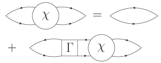
Figure 1: Bethe-Salpeter equation for the two-particle propagator.

Within the Dynamical Cluster Approximation (DCA) HTZ+98 ; MJPH05 , which we consider in this paper, one can consistently define the two-particle Green’s functions, by extracting the irreducible vertex function from the cluster. This approximation maps the original lattice problem to a cluster of size $L_{c}=l_{c}\times l_{c}$ embedded in a self-consistent host. Thus, correlations up to a range $\xi<l_{c}$ are treated accurately, while the physics at longer length-scales is described at the mean-field level. The DCA is conveniently formulated in momentum space, i.e. via a patching of the BZ. Let ${{\bm{K}}}$ denote such a patch, and ${{\bm{k}}}$ the original lattice momentum. The approximation boils down to restricting momentum conservation only to the patch wave vectors ${{\bm{K}}}$. This approximation is justified if $k$-space correlation functions are rather structureless and, thus, in real space short-ranged. From the technical point of view, the approximations are implemented via the Laue function $\Delta({{\bm{k}}_{1}},{{\bm{k}}_{2}},{{\bm{k}}_{3}},{{\bm{k}}_{4}})$, which guarantees momentum conservation up to a reciprocal lattice vector. In the DCA, the Laue function is replaced by $\Delta_{DCA}({{\bm{K}}_{1}},{{\bm{K}}_{2}},{{\bm{K}}_{3}},{{\bm{K}}_{4}})$, thereby insuring momentum conservation only between the cluster momenta. It is understood that ${{\bm{k}}}_{i}$ belongs to the patch ${{\bm{K}}}_{i}$.

To define uniquely the DCA approximation, in particular in view of two-particle quantities, it is useful to start with the Luttinger-Ward functional $\Phi$, which is computed using the DCA Laue function. Hence, $\Phi_{DCA}$ is a functional of a coarse-grained Green’s function, $\bar{G}({{\bm{K}}},i\omega_{m})\equiv\bar{G}(\underline{K})$. Irreducible quantities such as the self-energy, and the two-particle irreducible vertex are calculated on the cluster and correspond, respectively, to the first- and second-order functional derivatives of $\Phi_{DCA}$ with respect to $\bar{G}$. Using the cluster irreducible self-energy, $\Sigma({\underline{K}})$, and two-particle vertex, $\Gamma_{\underline{K}^{\prime},\underline{K}^{\prime\prime}}(\underline{Q})$, one can then compute the lattice single-particle and lattice two-particle correlation functions using the Dyson and Bethe-Salpeter equations. This construction of two-particle quantities has the appealing property that they are thermodynamically consistentBay62 ; BK61 . Hence, the spin susceptibility as calculated using the particle-hole correlation functions corresponds precisely to the derivative of the magnetization with respect to an applied uniform static magnetic field. The technical aspects of the above program are readily carried out for single-particle properties. However a full calculation of the irreducible two-particle vertex — even within the DCA — is prohibitively expensive JMHM01 and, thus, has never been carried out.

In the present work, we would like to overcome this situation by suggesting a scheme where the $\underline{K}^{\prime}-$ and $\underline{K}^{\prime\prime}-$ dependencies of the irreducible vertex are neglected. At low temperatures, this amounts to the assumption that in a energy and momentum window around the Fermi surface, the irreducible vertex depends weakly on $\underline{K}^{\prime}-$ and $\underline{K}^{\prime\prime}$. Following this assumption, an effective two-particle vertex in terms of an average over the $\underline{K}^{\prime}-$ and $\underline{K}^{\prime\prime}$ dependencies of $\Gamma_{\underline{K}^{\prime},\underline{K}^{\prime\prime}}(\underline{Q})$ is introduced:

$$\frac{1}{\beta L}U_{eff}(\underline{Q})=\langle\Gamma_{\underline{K}^{\prime},\underline{K}^{\prime\prime}}(\underline{Q})\rangle.$$ (4)

As shown in an earlier Quantum Monte Carlo (QMC) study by Bulut et al. (Ref. BSW93, ) for a single QMC cluster, this is reasonable for the 2D Hubbard model (on this QMC cluster of size $8\times 8$ with $U=8t$). The authors of Ref. BSW93, have also calculated with $U_{eff}(\underline{Q})$ the effective electron-electron interaction for the $8\times 8$ single QMC cluster. Both the momentum and frequency dependence were in rather good agreement with the QMC results for the effective electron-electron interaction.

Replacing the irreducible vertex by $\frac{1}{\beta L}U_{eff}(\underline{Q})$ in the cluster version of the Bethe-Salpeter Eq. (3) and carrying out the summations to obtain the cluster susceptibility gives:

$$U_{eff}(\underline{Q})=\frac{1}{\bar{\chi}_{0}(\underline{Q})}-\frac{1}{\chi(\underline{Q})},$$ (5)

where $\chi$ corresponds to the fully interacting susceptibility on the DCA cluster in the particle-hole channel and $\bar{\chi}_{0}$ is the corresponding bubble as obtained from the coarse-grained Green’s functions. Finally, our estimate of the lattice susceptibility reads:

$$\chi(\underline{q})=\frac{\chi_{0}(\underline{q})}{1-U_{eff}(\underline{Q})\cdot\chi_{0}(\underline{q})}.$$ (6)

where $\chi_{0}(\underline{q})$ corresponds to the bubble of the dressed lattice Green’s functions: $G(\underline{k})=\frac{1}{G_{0}^{-1}(\underline{k})-\Sigma(\underline{K})}$.

In the following section, we describe some aspects of the explicit implementation of the DCA which is based on the Hirsch-Fye QMC algorithm HF86 . Our new approach requires substantial testing. In Sec. III.1 we compare the Néel temperature as obtained within the DCA without any further approximations to the result obtained with our new approach. In Sec. III.2, we present results for the temperature and doping dependence of the spin and charge dynamical structure factors and compare the high temperature data with auxiliary field QMC simulations. Finally, Sec. IV draws conclusions.

II Implementation of the DCA

We consider the standard model of strongly correlated electron systems, the single-band Hubbard model Hub63 ; Gut63 ; Kan63

$$H=-\sum_{ij\sigma}t_{ij}c_{i\sigma}^{\dagger}c_{j\sigma}+U\sum_{i}n_{i\uparrow}n_{i\downarrow},$$ (7)

with hopping between nearest neighbors $t$ and Hubbard interaction $U$. The energy scale is set by $t$ and throughout the paper we consider $U=8t$.

Our goal is to compute the spin, $S({\bm{q}},\omega)$ and charge $C({\bm{q}},\omega)$ dynamical structure factors. They are given, respectively, by:

$$\langle S^{z}({\bm{q}},\tau)S^{z}(-{\bm{q}},0)\rangle=\frac{1}{\pi}\int{\rm d}w\;e^{-\tau\omega}\;S({\bm{q}},\omega)$$ (8a)

$$\langle N({\bm{q}},\tau)N(-{\bm{q}},0)\rangle=\frac{1}{\pi}\int{\rm d}w\;e^{-\tau\omega}\;C({\bm{q}},\omega).$$ (8b)

Here, $S^{z}({\bm{q}})=\frac{1}{\sqrt{L}}\sum_{{\bm{j}}}e^{i{\bm{q}}{\bm{j}}}\left(n_{j,\uparrow}-n_{j,\downarrow}\right)$ and $N({\bm{q}})=\frac{1}{\sqrt{L}}\sum_{{\bm{j}}}e^{i{\bm{q}}{\bm{j}}}\left(n_{j,\uparrow}+n_{j,\downarrow}\right)$ . The left hand side of the above equations are obtained from the corresponding susceptibility as calculated from Eq. (6). Finally, a stochastic version of the Maximum Entropy method Sandvik98 ; beach-2004 is used to extract the dynamical quantities.

In order to cross check our results, we slightly modify Eq. (6) to:

$$\chi(\underline{q})=\frac{\chi_{0}(\underline{q})}{1-\alpha\cdot U_{eff}(\underline{q})\cdot\chi_{0}(\underline{q})}.$$ (9)

Here, we have introduced an additional ”controlling” parameter $\alpha$ in the susceptibility denominator, which is calculated in a self-consistent manner. It assures, for example in the case of the longitudinal spin response, that $\chi(\underline{q})$ obeys the following sum rule (a similar idea, to use sumrules for constructing a controlled local approximation for the irreducible two-particle vertex has been implemented by Vilk and Tremblay (Ref. vilk97, )):

$$\frac{1}{\beta L}\sum_{\underline{q}}\chi(\underline{q})=\langle(S^{z}_{i})^{2}\rangle.$$ (10)

Of course, $\alpha$ should be as close as possible equal to $\alpha=1$, which is indeed what we will find after implementing the sum rule (see below).

Our implementation of the DCA for the Hubbard model is standard MJPH05 . Here, we will only discuss our interpolation scheme as well as the implementation of a SU(2)-spin symmetry broken algorithm. Since the DCA evaluates the irreducible quantities, $\Sigma(\underline{K})$ as well as $U_{eff}(\underline{Q})$ for the cluster wave vectors, an interpolation scheme has to be used. To this, we adopt the following strategy: for a fixed Matsubara frequency $i\Omega_{m}$ and for each cluster vector ${\bm{Q}}$, the effective interaction $U_{eff}$ is rewritten as a series expansion:

$$U_{eff}({\bm{Q}},i\Omega_{m})=\sum_{i}\sum_{\Delta_{i}}e^{i\Delta_{i}{\bm{Q}}}A_{i}(i\Omega_{m}),$$ (11)

with $i=0,...,n-1$, where $n$ is the number of the cluster momentum vectors ${\bm{Q}}$. The quantity $\Delta_{i}$ represents vectors, where each vector from the corresponding $\Delta_{i}$ belongs to the same ”shell” around the origin $(0,0)$ in real space, i.e.

$$\Delta_{0}=\left(\begin{array}[c]{c}0\\ 0\end{array}\right);\Delta_{1}=\pm\left(\begin{array}[c]{c}1\\ 0\end{array}\right),\pm\left(\begin{array}[c]{c}0\\ 1\end{array}\right)$$

$$\Delta_{2}=\left(\begin{array}[c]{c}\pm 1\\ \pm 1\end{array}\right),\left(\begin{array}[c]{c}\mp 1\\ \pm 1\end{array}\right);\Delta_{3}=\pm\left(\begin{array}[c]{c}2\\ 0\end{array}\right),\pm\left(\begin{array}[c]{c}0\\ 2\end{array}\right)...\;.$$

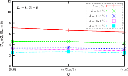
Figure 2: Static $(i\Omega_{m}=0)$ irreducible particle-hole interaction $U_{eff}$ for different cluster momentum vectors and dopings at inverse temperature $\beta t=6$ and $U=8t$.

With a given $U_{eff}$, Eq. (11) can be inverted to uniquely determine $A_{i}$. With these coefficients, one can compute the effective particle-hole interaction for every lattice momentum vector ${\bm{q}}$. This interpolation method works well when $U_{eff}$ is localized in real space and the sum in Eq. (11) can be cut-off at a given shell.

The effective particle-hole interaction $U_{eff}$ is shown in Fig. 2 for a variety of dopings at inverse temperature $\beta t=6$, $U/t=8$ and on an $L_{c}=8$ cluster, which corresponds to the so-called ”8A” Betts cluster (see Refs. BLF99, ; MJSKW05, ). The $U_{eff}$-function displays a smooth momentum dependence. These observations further support the interpolation scheme (Eq. 11). Thus, indeed, $U_{eff}$ is rather localized in real space with sizable reduction from its bare $U=8t$ value for larger doping and a further slight reduction at ${\bm{q}}=(\pi,\pi)$. The reduction is partly due to the self-energy effects in the single-particle propagator, which reduce $\bar{\chi}_{0}$ from its non-interacting ($U=0$) value $\chi^{(0)}$. Partly, it also reflects both the Kanamori (see Ref. Kan63, ) repeated particle-particle scattering and vertex corrections.

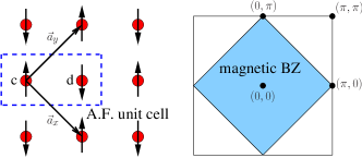
Figure 3: SU(2) symmetry broken DCA calculation. Left: A.F. unit cell with new basis vectors in realspace. Right: Reduced A.F. unit cell in momentum space.

Summarizing, the new approach to two-particle properties relies on two approximations which render the calculation of the corresponding Green’s function possible. Firstly, the effective particle-hole interaction $U_{eff}(\underline{Q})$ depends only on the center-of-mass momentum and frequency, i.e. ${\bm{Q}}$ and $i\Omega_{m}$. Secondly, $\chi(\underline{Q})$, is extracted directly from the cluster and $\bar{\chi}_{0}(\underline{Q})$ is obtained from the bubble of the coarse-grained Green’s functions.

To generate DCA results for the Néel temperature, we have used an SU(2) symmetry broken code. The setup is illustrated in Fig. 3. We introduce a doubling of the unit cell — to accommodate AF ordering — which in turn defines the magnetic Brillouin zone. The DCA k-space patching is carried out in the magnetic Brillouin zone and the Dyson equation for the single-particle propagator is given as a matrix equation:

$$G^{\sigma}(\underline{k})=\frac{1}{{G_{0}}^{-1}(\underline{k})-\Sigma^{\sigma}(\underline{K})},$$ (12)

with

$$G^{\sigma}(\underline{k})=\left(\begin{array}[c]{cc}G_{cc}^{\sigma}(\underline{k})&G_{cd}^{\sigma}(\underline{k})\\ G_{dc}^{\sigma}(\underline{k})&G_{dd}^{\sigma}(\underline{k})\end{array}\right).$$ (13)

With the SU(2) symmetry broken algorithm, one can compute directly the staggered magnetization, i.e. $m=\frac{1}{L}\sum_{{\bm{j}}}e^{i{\bm{Q}}{\bm{j}}}(n_{{\bm{j}},\uparrow}-n_{{\bm{j}},\downarrow})$, and thereby determine the transition temperature. Since the DCA is a conserving approximation, the so determined transition temperature corresponds precisely to the temperature scale at which the corresponding susceptibility, calculated without any approximations on the irreducible vertex $\Gamma_{\underline{K}^{\prime},\underline{K}^{\prime\prime}}(\underline{Q})$, diverges.

III Results

III.1 Comparison of the AF transition temperature with a symmetry broken DCA calculation

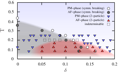
Figure 4: Phase diagram for the one-band Hubbard model with $U=8t$ with respect to different temperatures and fillings. The calculations are carried out on an $L_{c}=8$ cluster. The red and gray (blue and blank) objects indicate the antiferromagnetic (paramagnetic) phase. Shading of AF and PM regions is a guide to the eye. Details are in the text.

A first test of the validity of our new approach is a comparison with the SU(2) symmetry broken DCA calculation on an $L_{c}=8$ cluster at $U=8t$. The idea is to extract the Néel temperature $T_{N}$ from a divergence in the spin susceptibility as calculated in the above described (paramagnetic) scheme — see Eq. (9) — and to compare it to the DCA result as obtained from the SU(2) symmetry broken algorithm. This comparison provides information on the accuracy of our approximation to the two-particle irreducible vertex (see Eq. 4).

Using the SU(2) symmetry breaking algorithm, the magnetic phase diagram for the one-band Hubbard model as a function of doping is shown in Fig. 4. The para-(antiferro)magnetic phase transition is indicated here by gray (blank) circles. At half-filling $T_{N}\simeq 0.4t$ and magnetism survives up to approximately 15 % hole doping. It is know that the convergence of the magnetization during the self-consistent steps in the DCA approach is extremely poor near the phase transition and, therefore, we cannot estimate the transition temperature more precisely than shown in Fig. 4. However, our precision is sufficient for comparison. We again stress that the so determined magnetic phase diagram corresponds to the exact DCA result where no approximation — apart from coarse graining — is made on the particle-hole irreducible vertex.

The blue (red) triangles indicate the transition line for the para- to the antiferromagnetic solutions extracted from the divergent spin susceptibility (Eq. 9) within the paramagnetic calculation. A precise estimation of the N¸éel temperature requires very accurate results and boils down to finding the zeros of the denominator of Eq. (9). In Fig. 5, we consider the effective irreducible particle-hole interaction $U_{eff}$ for the static case and for the cluster momentum ${\bm{Q}}=(\pi,\pi)$ relevant for the AF instability. As apparent, the irreducible particle-hole interaction becomes weaker with increasing doping. On the other hand, the susceptibility $\chi_{0}({{\bm{q}}},i\Omega_{m}=0)$ grows with increasing doping. At a first glance both quantities $U_{eff}$ and $\chi_{0}$ (see Fig. 5) vary smoothly as a function of doping. However, in the vicinity of the phase transition, signalized by the vanishing of the denominator in Eq. (9), the precise interplay between $U_{eff}$ and $\chi_{0}$ becomes delicately important and renders an accurate estimate of the Néel temperature difficult. Given the difficulty in determining precisely the Néel temperature, we obtain good agreement between both methods at $\delta\gtrsim 10$ %. Note that in those calculations the values of $\alpha\approx 0.86-0.97$ are required to satisfy the sum rule in Eq. (10).

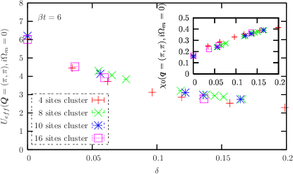
Figure 5: Static irreducible particle-hole interaction $U_{eff}$ for the cluster momentum vector ${\bm{Q}}=(\pi,\pi)$. The inset shows the static free lattice susceptibility $\chi_{0}$ for the momentum vector ${\bm{q}}=(\pi,\pi)$. The bare Hubbard interaction strength is $U=8t$.

At smaller dopings, and in particular at half-band filling the Néel temperature, as determined by the vanishing of the denominator in Eq. (9), underestimates the DCA result. Hence, in this limit, the $\underline{K}^{\prime}$ and $\underline{K}^{\prime\prime}$ dependence of the irreducible vertex plays an important role in the determination of $T_{N}$ and cannot be neglected.

Let us emphasize, that a good agreement between the Néel temperatures at $\delta\simeq 10$ % and above is a non-trivial achievement lending substantial support to the above new scheme for extracting two-particle Green’s functions.

III.2 Dynamical Spin and Charge structure factors

Figure 6: DCA (left) versus auxiliary field QMC (BSS) (right) for the dynamical spin and charge structure factors of the Hubbard model at $U/t=8$, $\delta\approx 14\;\%$ and $\beta t=3$. The BSS data on the $8\times 8$ lattice is essentially exact and acts as a benchmark for the DCA approach. The DCA calculations were carried out on an $L_{c}=8$ cluster. Here we have used $\alpha=0.98$ and $\alpha=1.01$ to satisfy the sum rule in the spin and charge sectors respectively.

To further asses the validity of our approach, we compare it to exact auxiliary-field Blankenbecler, Scalapino, Sugar (BSS) QMC results (Ref. preuss97, ). This method has a severe sign-problem especially in the vicinity of $\delta\simeq 10$ % and, hence, is restricted to high temperatures.

Such a comparison for the dynamical spin, $S({\bm{q}},\omega)$, and charge, $C({\bm{q}},\omega)$ dynamical structure factors is shown in Fig. 6 at $\beta t=3$, $\delta\approx 14\;\%$ and $U/t=8$. The BSS results correspond to simulations on an $8\times 8$ lattice. Fig. 6b) depicts the BSS-QMC data in the spin sector. Due to short-range spin-spin correlations, remnants of the spin-density-wave are observable, displaying a characteristic energy-scale of $2J$, where $J$ is the usual exchange coupling, i.e. $J=4\frac{t^{2}}{U}$. The two-particle DCA calculations show spin excitations with the dominant weight concentrated, as expected and seen in the QMC data, around the AF wavevector $(\pi,\pi)$. As apparent from the sum-rule,

$$\langle S^{z}({\bm{q}})S^{z}(-{\bm{q}})\rangle=\frac{1}{\pi}\int{\rm d}\omega\;S({\bm{q}},\omega)$$ (14)

(see Fig. 7 a)), the DCA overestimates the weight at this wave vector but does very well away from ${\bm{q}}=(\pi,\pi)$. The dispersion in the two-particle data has again a higher energy branch around $2J$, but it also shows features at $J$. Since the total spin is a conserved quantity, one expects a zero-energy excitation at ${\bm{q}}=(0,0)$. This is exactly reproduced in the $8\times 8$ QMC-BSS data, and qualitatively in the DCA results.

Figure 7: DCA a) versus BSS b) static spin correlation function at $U/t=8$, $\delta\approx 14\;\%$ and $\beta t=3$ on an $L_{c}=8$ cluster.

As a function of decreasing temperature, the DCA dynamical spin structure factor shows a more pronounced spin-wave spectrum. This is confirmed in Fig. 8 on the left hand side. Here, we fix the temperature to $\beta t=6$ and keep the doping at $\delta\approx 14\;\%$ but vary the cluster size. As apparent, for all considered cluster sizes ($L_{c}=4,8,10,16$) a spin wave feature is indeed observable: a peak maximum at ${\bm{q}}=(\pi,\pi)$ is present and the correct energy scale at ${\bm{q}}=(\pi,0)$ with $2J$ is recovered. Unfortunately, a direct comparison of both calculations at lower temperature is not possible due to the severe minus-sign problem in the BSS calculation.

Figure 8: Dynamical spin and charge structure factors of the Hubbard model at $\beta t=6$, $\delta\approx 14\;\%$ and $U/t=8$. for different cluster sizes: (a-b): $L_{c}=4$, (c-d): $L_{c}=8$, (e-f): $L_{c}=10$ and (g-h): $L_{c}=16$.

The investigation of the dynamical charge correlation function for the above parameters shows that the DCA calculations, which are depicted in Fig. 6 c), can also reproduce basic characteristics of the BSS charge excitation spectrum 6 d).

Table 1: Values of $\alpha$ for the spectra in Fig. 8.

Fig. 8	a,b	c,d	e,f	g,h
$\alpha$ (spin)	0.99	0.92	0.93	0.97
$\alpha$ (charge)	0.98	1.00	1.00	1.00

Both calculations show excitations at $\omega\approx U$ which are set by the remnants of the Mott-Hubbard gap. Similar results are obtained at lower temperatures ($\beta t=6$) on the right hand side of Fig. 8 for different cluster sizes ($L_{c}=4,8,10,16$). The corresponding values of $\alpha$ are listed in Tab. 1. These values confirm the overall correctness of our approach in that the corresponding sum rule for the charge response is accurately (exactly for $\alpha=1$) fulfilled.

The doping dependence of the spin- and charge-response is examined in Fig 9. Here, we restrict our calculations to the $L_{c}=8$ cluster at $\beta t=6$ and dopings between $\delta=14\;\%$ and $\delta=32\;\%$. At $\delta=14\;\%$ (see Fig. 8) the dynamical spin structure factor displays a spin wave dispersion with energy scale $J$. That is $E^{SDW}(\pi,0)=2J$ with $J=4\frac{t^{2}}{U}$. As the system is further doped ($\delta=27\;\%$) the dispersion is no longer sharply peaked around ${\bm{q}}=(\pi,\pi)$. The excitations broaden up and change their energy scale from $J=4\frac{t^{2}}{U}$ to an energy scale set by the non-interacting bandwidth. This effect becomes even more visible with higher dopings at $\delta=32\;\%$ (Fig. 9 c)). Furthermore, the spectrum of the charge response shows a reduction of the weight of states at high energies ($\omega/t\approx 8$). This behavior corresponds to the loss of weight of the upper Hubbard band with increasing doping. The corresponding equal time spin and charge correlation functions of Fig. 9 c-d) are depicted in Fig. 10. As in auxiliary-field QMC simulations IFT98 , the equal time spin correlation function shows a set of peaks at ${\bm{q}}=(\pi\pm\epsilon,\pi)$ and ${\bm{q}}=(\pi,\pi\pm\epsilon)$. Here $\epsilon$ is proportional to the doping. The overall trend of the doping dependence of the spin- and charge-responses is in good agreement with the previous findings of QMC simulations (Refs. preuss95, ; preuss97, ): there it was shown that the spin-response has a characteristic energy scale $\omega\approx 2J$ and an SDW-like dispersion up to about $\delta\approx 10-15$ % doping, despite the fact that at these dopings the spin-spin correlations are very short-ranged (of order of the lattice parameter).

A lot of the features of the two-particle spectra have direct influence on the single-particle spectral function and vice-versa. At optimal doping, $\delta=14$ % the spectral function $A({\bm{q}},\omega)$ in Fig. 11 a) shows three distinguish features. An upper Hubbard band ($\omega/t\approx 8t$) and a lower Hubbard band which splits in an incoherent background and a quasiparticle band of width set by the magnetic scale $J$.

Figure 9: Spin- and charge structure functions for different dopings: (a,b): 27 % and (c,d): 32 % The calculations are carried out on an $L_{c}=8$ cluster at $\beta t=6$.

In agreement with earlier QMC data (Refs. preuss95, ; preuss97, ), we view this narrow quasiparticle band as a fingerprint of a spin polaron where the bare particle is dressed by spin fluctuations. The fact that the dynamical spin structure factor in Fig 8 c)

Figure 10: Static spin a) and charge b) correlation function at $U/t=8$, $\delta\approx 32\;\%$ and $\beta t=6$ on an $L_{c}=8$ cluster.

shows a well defined magnon despersion at this temperature and doping, $\delta=14$ %, allows us to interpret the features centered around ${\bm{q}}=(0,0)$ and below the Fermi energy as backfolding or shadows of the quasiparticle band at ${\bm{q}}=(\pi,\pi)$. A comparison of the charge response spectrum in Fig. 8 d) with the corresponding single-particle spectra in Fig. 11 a) reveals that the response in the particle-hole channel at almost zero energy is caused by particle-hole excitations around the quasi-particle spin-polaron band close to the Fermi energy. The high energy excitations, mentioned above, are due to transitions from the quasi-particle band to the upper Hubbard band.

Figure 11: Angle-resolved spectral functions $A({\bm{q}},\omega)$ for various hole dopings: a): 14 %, b): 27 % and c): 32 %. Calculations are carried out on an $L_{c}=8$ cluster at $\beta t=6$.

As a function of doping, notable changes in the spectral function which are reflected in the two-particle properties are apparent. On one hand, the spectral weight in the upper Hubbard band is reduced. As mentioned previously, this reduction in high energy spectral weight is apparent in the dynamical charge structure factor. On the other hand, at higher dopings the magnetic fluctuations are suppressed. Consequently, the narrow band changes its bandwidth from the magnetic exchange energy $J$ to the free bandwidth. This evolution is clearly apparent in Figs. 11 b) and c) and is in good agreement with previous BSS-QMC results preuss97 .

IV Conclusions

Two-particle spectral functions, such as spin- and charge- dynamical spin structure factors, are clearly quantities which are of crucial relevance for the understanding of correlated materials. Within the DCA, those quantities have remained elusive due to numerical complexity. In principle, the two-particle irreducible vertex, $\Gamma_{\underline{K}^{\prime},\underline{K}^{\prime\prime}}(\underline{Q})$, containing three momenta and frequencies has to be extracted from the cluster and inserted in the Bethe-Salpeter equation. Calculating this quantity on the cluster is in principle possible, but corresponds to a daunting task which — to the best of our knowledge — has never been carried out. To circumvent this problem, we have proposed a simplification which relies on the assumption that $\Gamma_{\underline{K}^{\prime},\underline{K}^{\prime\prime}}(\underline{Q})$ is only weakly dependent on $\underline{K}^{\prime}$ and $\underline{K}^{\prime\prime}$. Given the validity of this assumption, one can average over $\underline{K}^{\prime}$ and $\underline{K}^{\prime\prime}$ and retain its dependency on frequency and momenta, $\underline{Q}$, of the excitation. We have tested this idea extensively for the two dimensional Hubbard model at strong couplings, $U/t=8$. At dopings $\delta\approx 10$ % and higher, we have found a good agreement between the Néel temperature on an $L_{c}=8$ lattice as calculated within a symmetry broken DCA scheme with our new two-particle approach. This finding lends support to the validity of our scheme in this doping range. Furthermore, we studied the doping and temperature dependence of the spin and charge dynamical structure factors as well as the single-particle spectral function at $\beta t=6$. Our results provide a consistent picture of the physics of doped Mott insulators, very reminiscent of previous findings within auxiliary field QMC simulations. The strong point of the method, in contrast to auxiliary field QMC approaches, is that it can be pushed to lower temperatures above and below the superconducting transition temperature. Work in this direction is presently under progress.

- (1) A. Damascelli, Z. Hussain, and Z.-X. Shen, Rev. Mod. Phys. 75, 473 (2003).
- (2) R. Preuss, W. Hanke, and W. von der Linden, Phys. Rev. Lett. 75, 1344 (1995).
- (3) R. Preuss, W. Hanke, C. Gröber, and H. G. Evertz, Phys. Rev. Lett. 79, 1122 (1997).
- (4) M. Imada, A. Fujimori, and Y. Tokura, Rev. Mod. Phys. 68, 13 (1998).
- (5) M. H. Hettler, A. N. Tahvildar-Zadeh, M. Jarrell, T. Pruschke, and H. R. Krishnamurthy, Phys. Rev. B 58, R7475 (1998).
- (6) T. Maier, M. Jarrell, T. Pruschke, and M. H. Hettler, Rev. Mod. Phys. 77, 1027 (2005).
- (7) G. Baym, Phys. Rev. 127, 1391 (1962).
- (8) G. Baym and L. P. Kadanoff, Phys. Rev. 124, 287 (1961).
- (9) M. Jarrell, T. Maier, C. Huscroft, and S. Moukouri, Phys. Rev. B 64, 195130 (2001).
- (10) N. Bulut, D. J. Scalapino, and S. R. White, Phys. Rev. B 47, 2742 (1993).
- (11) J. E. Hirsch and R. M. Fye, Phys. Rev. Lett. 56, 2521 (1986).
- (12) J. Hubbard, Proc. R. Soc. London A 276, 238 (1963).
- (13) M. C. Gutzwiller, Phys. Rev. Lett. 10, 159 (1963).
- (14) J. Kanamori, Prog. Theor. Phys. (Kyoto) 30, 275 (1963).
- (15) A. Sandvik, Phys. Rev. B 57, 10287 (1998).
- (16) K. S. D. Beach, 2004, arXiv:cond-mat/0403055.
- (17) Y. Vilk and A.-M. Tremblay, J. de Physique 7, 1309 (1997).
- (18) D. Betts, H. Lin, and J. Flynn, Can. J. Phys. 77, 353 (1999).
- (19) T. Maier, M. Jarrell, T. Schulthess, P. Kent, and J. White, Phys. Rev. Lett. 95, 237001 (2005).