On the condensed density of the generalized eigenvalues of pencils of Gaussian random matrices and applications

P. Barone Istituto per le Applicazioni del Calcolo ”M. Picone”, C.N.R.,
Via dei Taurini 19, 00185 Rome, Italy
e-mail: piero.barone@gmail.com, p.barone@iac.cnr.it
fax: 39-6-4404306

Abstract

Pencils of matrices whose elements have a joint noncentral Gaussian distribution with nonidentical covariance are considered. An approximation to the distribution of the squared modulus of their determinant is computed which allows to get a closed form approximation of the condensed density of the generalized eigenvalues of the pencils. Implications of this result for solving several moments problems are discussed and some numerical examples are provided.

Key words: random determinants, complex exponentials, complex moments problem, logarithmic potentials

Introduction

Let us define the random Hankel matrices

$\displaystyle{\bf U}_{0}=\left[\begin{array}[]{llll}{\bf a}_{0}&{\bf a}_{1}&\dots&{\bf a}_{p-1}\\ {\bf a}_{1}&{\bf a}_{2}&\dots&{\bf a}_{p}\\ .&.&\dots&.\\ {\bf a}_{p-1}&{\bf a}_{p}&\dots&{\bf a}_{n-2}\end{array}\right],\;\;{\bf U}_{1}=\left[\begin{array}[]{llll}{\bf a}_{1}&{\bf a}_{2}&\dots&{\bf a}_{p}\\ {\bf a}_{2}&{\bf a}_{3}&\dots&{\bf a}_{p+1}\\ .&.&\dots&.\\ {\bf a}_{p}&{\bf a}_{p+1}&\dots&{\bf a}_{n-1}\end{array}\right]$ (9)

where n=2​p,𝐚k=sk+Ο΅k,k=0,1,2,…,nβˆ’1,Ο΅kformulae-sequence𝑛2𝑝formulae-sequencesubscriptπšπ‘˜subscriptπ‘ π‘˜subscriptbold-italic-Ο΅π‘˜π‘˜012…𝑛1subscriptbold-italic-Ο΅π‘˜n=2p,\;\;{\bf a}_{k}=s_{k}+{\mbox{\boldmath$\epsilon$}}_{k},\quad k=0,1,2,\dots,n-1,\;\;{\mbox{\boldmath$\epsilon$}}_{k} is a complex Gaussian, zero mean, white noise, with variance Οƒ2superscript𝜎2\sigma^{2} and sk∈I​Csubscriptπ‘ π‘˜πΌπΆs_{k}\in I\!\!\!\!{C}. In the following all random quantities are denoted by bold characters. Let us consider the generalized eigenvalues {𝝃j,j=1,…,p}formulae-sequencesubscript𝝃𝑗𝑗1…𝑝\{{\mbox{\boldmath$\xi$}}_{j},\;j=1,\dots,p\} of (𝐔1,𝐔0)subscript𝐔1subscript𝐔0({\bf U}_{1},{\bf U}_{0}) i.e. the roots of the polynomial 𝐏​(z)=det[(𝐔1βˆ’z​𝐔0)]𝐏𝑧delimited-[]subscript𝐔1𝑧subscript𝐔0{\bf P}(z)=\det[({\bf U}_{1}-z{\bf U}_{0})], which form a set of exchangeable random variables. Their marginal density h​(z)β„Žπ‘§h(z) also called condensed density [14] or normalized one-point correlation function [12], is the expected value of the (random) normalized counting measure on the zeros of 𝐏​(z)𝐏𝑧{\bf P}(z) i.e.

$$h(z)=\frac{1}{p}E\left[\sum_{j=1}^{p}\delta(z-{\mbox{\boldmath$\xi$}}_{j})\right]$$

or, equivalently, for all Borel sets $A\subset I\!\!\!\!{C}$

$$\int_{A}h(z)dz=\frac{1}{p}\sum_{j=1}^{p}Prob({\mbox{\boldmath$\xi$}}_{j}\in A).$$

It can be proved that (see e.g. [4]) $h(z)=\frac{1}{4\pi}\Delta u(z)$ where $\Delta$ denotes the Laplacian operator with respect to $x,y$ if $z=x+iy$ and $u(z)=\frac{1}{p}E\left\{\log(|{\bf P}(z)|^{2})\right\}$ is the corresponding logarithmic potential.

The condensed density $h(z)$ plays an important role for solving moment problems such as the trigonometric, the complex, the Hausdorff ones. It was shown in $[2-10]$, [17, 18] that all these problems can be reduced to the complex exponentials approximation problem (CEAP), which can be stated as follows. Let us consider a uniformly sampled signal made up of a linear combination of complex exponentials

sk=βˆ‘j=1pβˆ—cj​ξjk.subscriptπ‘ π‘˜superscriptsubscript𝑗1superscript𝑝subscript𝑐𝑗superscriptsubscriptπœ‰π‘—π‘˜\displaystyle s_{k}=\sum_{j=1}^{p^{*}}c_{j}\xi_{j}^{k}. (10)

where $c_{j},\xi_{j}\in I\!\!\!\!{C}.$ Let us assume to know an even number $n=2p,\;p\geq{p^{*}}$ of noisy samples

𝐚k=sk+Ο΅k,k=0,1,2,…,nβˆ’1formulae-sequencesubscriptπšπ‘˜subscriptπ‘ π‘˜subscriptbold-italic-Ο΅π‘˜π‘˜012…𝑛1{\bf a}_{k}=s_{k}+{\mbox{\boldmath$\epsilon$}}_{k},\quad k=0,1,2,\dots,n-1

where ${\mbox{\boldmath$\epsilon$}}_{k}$ is a complex Gaussian, zero mean, white noise, with finite known variance $\sigma^{2}$. We want to estimate ${p^{*}},c_{j},\xi_{j},\;j=1,\dots,{p^{*}}$, which is a well known ill-posed inverse problem. We notice that, in the noiseless case and when $p={p^{*}}$, the parameters $\xi_{j}$ are the generalized eigenvalues of the pencil $(U_{1},U_{0})$ where now $U_{0}$ and $U_{1}$ are built as in (9) but starting from {sk}.subscriptπ‘ π‘˜\{s_{k}\}.

From its definition it is evident that the condensed density provides information about the location in the complex plane of the generalized eigenvalues of $({\bf U}_{1},{\bf U}_{0})$ whose estimation is the most difficult part of CEAP. Unfortunately its computation is very difficult in general. In [10] a method to solve CEAP was proposed based on an approximation of the condensed density. An explicit expression of $h(z)$ proposed by Hammersley [14] when the coefficients of ${\bf P}(z)$ are jointly Gaussian distributed was used. The second order statistics of these coefficients in the CEAP case were estimated by computing many Pade’ approximants of different orders to the $Z$-transform of the data $\{{\bf a}_{k}\}$. This last step was essential to realize the averaging that appears in the definition of $h(z)$, which is the key feature to make the condensed density a useful tool for applications. In fact in the noiseless case $h(z)$ is a sum of Dirac $\delta$ distributions centered on the generalized eigenvalues while, when the signal is absent (sk=0β€‹βˆ€ksubscriptπ‘ π‘˜0for-allπ‘˜s_{k}=0\;\;\forall k), it was proved in [4] that if $z=re^{i\theta}$, the marginal condensed density $h^{(r)}(r)$ w.r. to $r$ of the generalized eigenvalues is asymptotically in $n$ a Dirac $\delta$ supported on the unit circle $\forall\sigma^{2}$. Moreover for finite $n$ the marginal condensed density w.r. to $\theta$ is uniformly distributed on $[-\pi,\pi]$. Therefore if the signal-to-noise ratio (e.g. $SNR=\frac{1}{\sigma}\min_{h=1,{p^{*}}}|c_{h}|$) is large enough $h(z)$ has local maxima in a neighbor of each $\xi_{j},\;j=1,\dots,{p^{*}}$ and this fact can be exploited to get good estimates of $\xi_{j}$. However usually we have only one realization of the discrete process $\{{\bf a}_{k}\}$, hence we cannot estimate $h(z)$ by averaging. In [3] a stochastic perturbation method is proposed to overcome this problem. It is based on the computation of the generalized eigenvalues of many pencils obtained by suitable perturbations of the measured one. The computational burden is therefore relevant. We then look for an approximation of $h(z)$ which can be well estimated by a single realization of $\{{\bf a}_{k}\}$. It turns out that the proposed approximation holds for pencils made up by random matrices whose elements have a joint Gaussian distribution. However the specific algebraic structure of CEAP, which gives rise to pencils of Hankel random matrices, can be taken into account to further reduce the computational burden. Moreover it will be shown that the noise contribution to $h(z)$ can be smoothed out to some extent simply acting on a parameter of the approximant.

The paper is organized as follows. In Section 1 some algebraic and statistical preliminaries are developed. In Section 2 the closed form approximation of $h(z)$ is defined in the general case. In Section 3 it is shown how to get a smooth estimate of $h(z)$ from the data by exploiting its closed form approximation in the Hankel case. In Section 4 computational issues are discussed in the Hankel case. Finally in Section 5 some numerical examples are provided.

1 Preliminaries

Let us consider the $p\times p$ complex random pencil ${\bf G}(z)={\bf G}_{1}-z{\bf G}_{0},\;\;z\in I\!\!\!\!{C}$ where the elements of $\Re{{\bf G}_{0}},\Im{{\bf G}_{0}},\Re{{\bf G}_{1}},\Im{{\bf G}_{1}}$ have a joint Gaussian distribution and $\Re$ and $\Im$ denotes the real and imaginary parts. Dropping the dependence on $z$ for simplifying the notations, let us define

$${\bf G}=[{\underline{\bf g}}_{1},\dots,{\underline{\bf g}}_{p}],\;\;\;{\underline{\bf g}}=vec({\bf G})=[{\underline{\bf g}}_{1}^{T},{\underline{\bf g}}_{2}^{T},\dots,{\underline{\bf g}}_{p}^{T}]^{T}$$

Moreover $\forall z$, let us define 𝐠¯ˇk=[β„œβ‘π Β―kT,ℑ⁑𝐠¯kT]TsubscriptΛ‡Β―π π‘˜superscriptsuperscriptsubscriptΒ―π π‘˜π‘‡superscriptsubscriptΒ―π π‘˜π‘‡π‘‡\check{{\underline{\bf g}}}_{k}=[\Re{{\underline{\bf g}}_{k}}^{T},\Im{{\underline{\bf g}}_{k}}^{T}]^{T} and

$$\check{{\underline{\bf g}}}=[\check{{\underline{\bf g}}}_{1}^{T},\check{{\underline{\bf g}}}_{2}^{T},\dots,\check{{\underline{\bf g}}}_{p}^{T}]^{T}.$$

Then $\check{{\underline{\bf g}}}$ will have a multivariate Gaussian distribution with mean ${\underline{\mu}}=E[\check{{\underline{\bf g}}}]\in I\!\!R^{2p^{2}}$ and covariance $\Sigma\in I\!\!R^{2p^{2}\times 2p^{2}}$. We notice that no independence assumption neither between elements of ${\bf G}_{0}$ and ${\bf G}_{1}$ nor between real and imaginary parts is made. Hence this is the most general hypothesis that can be done about the Gaussian distribution of the complex random vector ${\underline{\bf g}}$, (see [21] for a full discussion of this point).

Let us consider the $QR$ factorization of ${\bf G}$ where ${\bf Q}^{H}{\bf Q}={\bf Q}{\bf Q}^{H}=I_{p}$ where $H$ denotes transposition plus conjugation, ${\bf R}$ is an upper triangular matrix and $I_{p}$ is the identity matrix of order $p$. We then have

$$|\det({\bf G})|^{2}=|\det({\bf Q}{\bf R})|^{2}=|\det({\bf R})|^{2}=\prod_{k=1,p}|{\bf R}_{kk}|^{2}.$$

We want to compute the condensed density of the generalized eigenvalues of the pencil ${\bf G}(z)$ which is given by [14, 4]:

$$h(z)=\frac{1}{4\pi p}\Delta E\left\{\log(|det[{\bf G}(z)]|^{2})\right\}=\frac{1}{4\pi p}\Delta\sum_{k=1}^{p}E\left\{\log|{\bf R}_{kk}(z)|^{2}\right\}.$$

We are therefore interested on the distribution of $|{\bf R}_{kk}|^{2},k=1,\dots,p$ in order to compute $E[\log|{\bf R}_{kk}|^{2}]$.

To perform the $QR$ factorization of the random matrix ${\bf G}$ we can use the Gram-Schmidt algorithm. If ${\bf Q}=[{\underline{\bf q}}_{1},\dots,{\underline{\bf q}}_{p}]$ it is given in Table 1.

For $k=1,\dots,p$
      𝐰¯k=𝐠¯ksubscriptΒ―π°π‘˜subscriptΒ―π π‘˜{\underline{\bf w}}_{k}={\underline{\bf g}}_{k}
Β Β Β Β Β Β if $k>1$ then
         𝐑i​k=πͺΒ―iH​𝐠¯k,i=1,…,kβˆ’1formulae-sequencesubscriptπ‘π‘–π‘˜superscriptsubscriptΒ―πͺ𝑖𝐻subscriptΒ―π π‘˜π‘–1β€¦π‘˜1{\bf R}_{ik}={\underline{\bf q}}_{i}^{H}{\underline{\bf g}}_{k},\;i=1,\dots,k-1
         ${\underline{\bf w}}_{k}={\underline{\bf w}}_{k}-\sum_{i=1}^{k-1}{\bf R}_{ik}{\underline{\bf q}}_{i}$
Β Β Β Β Β Β end
         ${\bf R}_{kk}=\sqrt{{\underline{\bf w}}_{k}^{H}{\underline{\bf w}}_{k}}$
Β Β Β Β Β Β Β Β Β πͺΒ―k=𝐰¯k𝐑k​ksubscriptΒ―πͺπ‘˜subscriptΒ―π°π‘˜subscriptπ‘π‘˜π‘˜{\underline{\bf q}}_{k}=\frac{{\underline{\bf w}}_{k}}{{\bf R}_{kk}}
end
Table 1: The Gram-Schmidt algorithm

We notice that $|{\bf R}_{kk}|={\bf R}_{kk}$ and

𝐑k​k2={𝐠¯kH​𝐠¯k,Β ifΒ k=1𝐠¯kH​(Ipβˆ’βˆ‘i=1kβˆ’1πͺΒ―i​πͺΒ―iH)​𝐠¯k,Β ifΒ k>1superscriptsubscriptπ‘π‘˜π‘˜2casessuperscriptsubscriptΒ―π π‘˜π»subscriptΒ―π π‘˜Β ifΒ k=1missing-subexpressionmissing-subexpressionmissing-subexpressionsuperscriptsubscriptΒ―π π‘˜π»subscript𝐼𝑝superscriptsubscript𝑖1π‘˜1subscriptΒ―πͺ𝑖superscriptsubscriptΒ―πͺ𝑖𝐻subscriptΒ―π π‘˜Β ifΒ k>1missing-subexpressionmissing-subexpressionmissing-subexpression{\bf R}_{kk}^{2}=\left\{\begin{array}[]{llll}{\underline{\bf g}}_{k}^{H}{\underline{\bf g}}_{k},\mbox{ if $k=1$}\\ {\underline{\bf g}}_{k}^{H}\left(I_{p}-\sum_{i=1}^{k-1}{\underline{\bf q}}_{i}{\underline{\bf q}}_{i}^{H}\right){\underline{\bf g}}_{k},\mbox{ if $k>1$}\end{array}\right.

where ${\underline{\bf q}}_{i}$ are functions of ${\underline{\bf g}}_{j},\;j=1,\dots,i$. Therefore, denoting by 𝐠¯~k={𝐠¯ˇ1,…,𝐠¯ˇkβˆ’1}subscript~Β―π π‘˜subscriptˇ¯𝐠1…subscriptΛ‡Β―π π‘˜1\tilde{{\underline{\bf g}}}_{k}=\{\check{{\underline{\bf g}}}_{1},\dots,\check{{\underline{\bf g}}}_{k-1}\} we have that

$$\left\{\begin{array}[]{llll}{\bf R}_{11}^{2}\mbox{ is a quadratic form in Gaussian variables}\\ {\bf R}_{kk}^{2},\;k>1,\mbox{ conditioned on $\tilde{{\underline{\bf g}}}_{k}$, is a quadratic form in Gaussian variables }.\end{array}\right.$$

Moreover let us denote by ${\underline{e}}_{k}$ the $k-$th column of $I_{p}$ and let be $E_{k}={\underline{e}}_{k}\otimes I_{2p}$ then ${\underline{\mu}}_{k}=E_{k}^{T}{\underline{\mu}},\;\;\Sigma_{k}=E_{k}^{T}\Sigma E_{k}$ are the mean vector and covariance matrix of 𝐠¯ˇksubscriptΛ‡Β―π π‘˜\check{{\underline{\bf g}}}_{k}. Then we have

Lemma 1

For $k=1$ and for $k>1$, conditioned on 𝐠¯~ksubscript~Β―π π‘˜\tilde{{\underline{\bf g}}}_{k}, ${\bf R}_{kk}^{2}$ is distributed as $\sum_{r=1}^{n}\lambda^{(k)}_{r}\chi^{2}_{\nu_{r}}(\delta_{r})$, $n=2p$, and $\chi^{2}_{\nu_{r}}(\delta_{r})$ are independent, where $2(p-k+1)=\sum_{r=1}^{n}\nu_{r}\;$, $\lambda^{(k)}_{r}$ are the distinct eigenvalues of $\Sigma_{k}^{1/2}{\mathcal{R}({\bf A}_{k})}\Sigma_{k}^{1/2}\;\;$ with multiplicity $\nu_{r}$, ${\underline{u}}^{(k)}_{i},\;i=1,\dots,n$ are the corresponding eigenvectors, $\delta_{r}=\sum_{(r)}({\underline{u}}^{(k)}_{i})^{T}\Sigma_{k}^{-1/2}{\underline{\mu}}_{k})^{2},$ the summation being over all eigenvectors corresponding to eigenvalue $\lambda^{(k)}_{r}$,

$${\bf A}_{k}=(I_{p}-\sum_{i=1}^{k-1}{\underline{\bf q}}_{i}{\underline{\bf q}}_{i}^{H})$$

and

$${\mathcal{R}({\bf A}_{k})}=\left[\begin{array}[]{rrrr}\Re({\bf A}_{k})&\;\;-\Im({\bf A}_{k})\\ \Im({\bf A}_{k})&\;\;\Re({\bf A}_{k})\end{array}\right]$$

with $-\Im({\bf A}_{k})=\Im({\bf A}_{k})^{T}$ is the real isomorph of ${\bf A}_{k}.$

proof. ${\bf A}_{k}=\Re({\bf A}_{k})+i\Im({\bf A}_{k})$ is hermitian and idempotent because ${\underline{\bf q}}_{i}$ are orthonormal vectors. Therefore $\mbox{rank}({\bf A}_{k})=p-k+1$ and $\mbox{rank}({\mathcal{R}({\bf A}_{k})})=2(p-k+1)$ because the eigenvalues of ${\mathcal{R}({\bf A}_{k})}$ are those of ${\bf A}_{k}$ with multiplicity $2$. As ${\bf A}_{k}$ depends only on ${\underline{\bf q}}_{i},\;i=1,\dots,k-1$ which in turn depend only on ${\underline{\bf g}}_{i},\;i=1,\dots,k-1$ it follows that, conditioned on 𝐠¯~ksubscript~Β―π π‘˜\tilde{{\underline{\bf g}}}_{k}, ${\mathcal{R}({\bf A}_{k})}$ is a constant matrix. Moreover 𝐠¯kH​𝐀k​𝐠¯k=𝐠¯ˇkT​ℛ​(𝐀k)​𝐠¯ˇksuperscriptsubscriptΒ―π π‘˜π»subscriptπ€π‘˜subscriptΒ―π π‘˜superscriptsubscriptΛ‡Β―π π‘˜π‘‡β„›subscriptπ€π‘˜subscriptΛ‡Β―π π‘˜{\underline{\bf g}}_{k}^{H}{\bf A}_{k}{\underline{\bf g}}_{k}=\check{{\underline{\bf g}}}_{k}^{T}{\mathcal{R}({\bf A}_{k})}\check{{\underline{\bf g}}}_{k} as can be easily checked. Let us define the variables xΒ―=(U(k))Tβ€‹Ξ£βˆ’1/2​𝐠¯ˇkΒ―π‘₯superscriptsuperscriptπ‘ˆπ‘˜π‘‡superscriptΞ£12subscriptΛ‡Β―π π‘˜{\underline{x}}=(U^{(k)})^{T}\Sigma^{-1/2}\check{{\underline{\bf g}}}_{k}. We have 𝐠¯ˇkT​ℛ​(𝐀k)​𝐠¯ˇk=xΒ―T​Λ(k)​xΒ―superscriptsubscriptΛ‡Β―π π‘˜π‘‡β„›subscriptπ€π‘˜subscriptΛ‡Β―π π‘˜superscriptΒ―π‘₯𝑇superscriptΞ›π‘˜Β―π‘₯\check{{\underline{\bf g}}}_{k}^{T}{\mathcal{R}({\bf A}_{k})}\check{{\underline{\bf g}}}_{k}={\underline{x}}^{T}\Lambda^{(k)}{\underline{x}} where $\Lambda^{(k)}$ is the diagonal matrix of eigenvalues of $\Sigma_{k}^{1/2}{\mathcal{R}({\bf A}_{k})}\Sigma_{k}^{1/2}$. Only $m_{k}=2(p-k+1)$ eigenvalues are not zero and we can assume that they are the first $m_{k}$. Therefore ${\bf R}_{kk}^{2}=\sum_{i=1}^{m_{k}}\lambda^{(k)}_{i}{\underline{x}}_{i}^{2}$ is a quadratic form in Gaussian vectors of dimension $m_{k}$. The thesis follows e.g. by [16, ch.29,sec.4]. $\Box$

Corollary 1

If $\Sigma=I_{2p^{2}}$ and ${\underline{\mu}}=0$, ${\bf R}_{kk}^{2}$ is distributed as $\chi^{2}_{2(p-k+1)}$

proof. As $\Sigma=I_{2p^{2}}$ the eigenvalues of $\Sigma_{k}^{1/2}{\mathcal{R}({\bf A}_{k})}\Sigma_{k}^{1/2}$ are those of ${\mathcal{R}({\bf A}_{k})}$ which are $1$ with multiplicity $2(p-k+1)$ and 00 with multiplicity $2(k-1)$. As ${\underline{\mu}}=0$, $\delta_{i}=0$. Remembering that the $\chi^{2}_{1}(\delta_{i})$ appearing in the previous Lemma are independent, the thesis follows by the additivity property of $\chi^{2}$ distribution . $\Box$

Remark. The Corollary follows also by Bartlett’s decomposition of a i.i.d. zero mean Gaussian random matrix [11].

2 Closed form approximation of $h(z)$

Unfortunately we cannot use the easy result stated in the Corollary because in the case of interest the matrix ${\bf G}(z)$ has a mean different from zero and a covariance structure depending on $z$. By Lemma 1 we know that ${\bf R}_{11}^{2}$ is distributed as a linear combination of non-central $\chi^{2}$ distributions. It is known that this distribution admits an expansion $\mathcal{L}\left(\alpha,\beta,\tau\right)$ in series of generalized Laguerre polynomials [16, ch.29,sec.6.3] and the series is uniformly convergent in $I\!\!R^{+}$. More specifically let us denote the generalized Laguerre polynomial of order $m$ by

$$L_{m}(x,\alpha)=\frac{x^{-(\alpha-1)}e^{x}}{m!}\frac{\partial^{m}}{\partial x^{m}}(x^{m+\alpha-1}e^{-x})=\sum_{h=0}^{m}c_{hm}x^{h}$$

where

$$c_{hm}=\frac{(-1)^{h}\Gamma(\alpha+m)}{h!(m-h)!\Gamma(\alpha+h)}.$$

Then, following [22], we have

Lemma 2

The density function of ${\bf R}_{11}^{2}$ is given by

$$f_{1}(y)=b_{0}\frac{y^{\alpha-1}e^{-y/\beta}}{\beta^{\alpha}\Gamma(\alpha)}+\frac{y^{\alpha-1}e^{-y/\beta}}{\beta^{\alpha}\Gamma(\alpha)}\sum_{m=1}^{\infty}b_{m}L_{m}(y/\tau,\alpha)=\mathcal{L}\left(\alpha,\beta,\tau\right)$$

where $\alpha$ and $\beta$ are such that the first two moments of ${\bf R}_{11}^{2}$ are the same of the first two moments of the gamma distribution representing the leading term of the expansion. Moreover $b_{m}$ are univocally determined by the moments and $\tau$ is a free parameter. If $\lambda_{max}$ denotes the maximum eigenvalue of $\Sigma_{1}$, when $\tau^{-1}>2(\beta^{-1}-(2\lambda_{max})^{-1})$ the series $\mathcal{L}\left(\alpha,\beta,\tau\right)$ is uniformly convergent $\forall y\in I\!\!R^{+}.$ If $\beta>\lambda_{max}$ then $\tau=\beta$ makes the series to converge uniformly, $b_{0}=1$ and $b_{m}$ are determined by the first $m$ moments of ${\bf R}_{11}^{2}$.

proof. The proof follows by the results given in [22] for the distribution of quadratic forms in central normal variables which hold true also in the non-central case as can be easily checked. $\Box$

We can compute $E[\log({\bf R}_{11}^{2})]$ by

Lemma 3
$\displaystyle E[\log({\bf R}_{11}^{2})]=b_{0}[\log\beta+\Psi(\alpha)]$
$\displaystyle+$ $\displaystyle\sum_{m=1}^{\infty}b_{m}\sum_{h=0}^{m}c_{hm}\frac{\Gamma(\alpha+h)}{\Gamma(\alpha)}\left(\frac{\beta}{\tau}\right)^{h}\left[\log\beta+\Psi(\alpha+h)\right]$

proof. By Lemma 2 the series $\mathcal{L}\left(\alpha,\beta,\tau\right)$ converges uniformly. Therefore term-by-term integration can be performed and the result follows by noticing that, for $h=0,1,\dots$

$$\frac{1}{\beta^{\alpha}}\int_{0}^{\infty}\log(y)\left(\frac{y}{\tau}\right)^{h}y^{\alpha-1}e^{-y/\beta}dy=\Gamma(\alpha+h)\left(\frac{\beta}{\tau}\right)^{h}\left[\log\beta+\Psi(\alpha+h)\right].$$

$\Box$

We have then obtained a closed form expression for $E[\log({\bf R}_{11}^{2})]$ as a function of the moments of ${\bf R}_{11}^{2}$. By noticing that the same result holds true for the distribution of ${\bf R}_{kk}^{2}$ conditioned on 𝐠¯~ksubscript~Β―π π‘˜\tilde{{\underline{\bf g}}}_{k}, we show now how to get an approximation of $E[\log({\bf R}_{kk}^{2})],\;k>1$.

Theorem 1

The density function $f_{k}(y)$ of ${\bf R}_{kk}^{2}$ can be expanded in a uniformly convergent series of Laguerre functions

$$f_{k}(y)=b^{(k)}_{0}\frac{y^{\alpha_{k}-1}e^{-y/\beta_{k}}}{\beta_{k}^{\alpha_{k}}\Gamma(\alpha_{k})}+\frac{y^{\alpha_{k}-1}e^{-y/\beta_{k}}}{\beta_{k}^{\alpha_{k}}\Gamma(\alpha_{k})}\sum_{m=1}^{\infty}b^{(k)}_{m}L_{m}(y/\tau_{k},\alpha_{k}).$$

When the parameter $\tau_{k}$, that controls the uniform convergence of the series, can be chosen equal to $\beta_{k}$, then $b^{(k)}_{0}=1$ and $b^{(k)}_{m},\;m=0,\dots,N$ depends on the first $N+1$ moments of ${\bf R}_{kk}^{2}$. Moreover

$\displaystyle E[\log({\bf R}_{kk}^{2})]=b^{(k)}_{0}[\log\beta_{k}+\Psi(\alpha_{k})]+$
$\displaystyle\sum_{m=1}^{\infty}b^{(k)}_{m}\sum_{h=0}^{m}c_{hm}\frac{\Gamma(\alpha_{k}+h)}{\Gamma(\alpha_{k})}\left(\frac{\beta_{k}}{\tau_{k}}\right)^{h}\left[\log\beta_{k}+\Psi(\alpha_{k}+h)\right].$

If the series is truncated after $N+1$ terms, the approximation error

$\displaystyle\eta_{N}^{(k)}$ $\displaystyle=$ $\displaystyle\left|E[\log({\bf R}_{kk}^{2})]-\left(b^{(k)}_{0}[\log\beta_{k}+\Psi(\alpha_{k})]\right.\right.+$
$\displaystyle\left.\left.\sum_{m=1}^{N}b^{(k)}_{m}\sum_{h=0}^{m}c_{hm}\frac{\Gamma(\alpha_{k}+h)}{\Gamma(\alpha_{k})}\left(\frac{\beta_{k}}{\tau_{k}}\right)^{h}\left[\log\beta_{k}+\Psi(\alpha_{k}+h)\right]\right)\right|$

is bounded by

$\displaystyle K_{1}\frac{\epsilon^{N+1}}{\alpha_{k}^{2}\beta_{k}^{\alpha_{k}}\Gamma(\alpha_{k})}\left({{}_{2}F_{2}}\left(\alpha_{k},\alpha_{k};1+\alpha_{k},1+\alpha_{k};K_{2}\right)+G^{3,0}_{0,2}\left(-K_{2}\left|\stackrel{{\scriptstyle 1-\alpha_{k},1-\alpha_{k}}}{{\scriptstyle 0,-\alpha_{k},-\alpha_{k}}}\right.\right)\right)$

where $K_{1}>0,\;K_{2}>0$ and $0<\epsilon<1$ are constants, ${}_{2}F_{2}$ is a generalized hypergeometric function and $G^{3,0}_{0,2}$ is a Meijer’s G-function.

proof. By Lemma 1, conditioned on 𝐠¯~ksubscript~Β―π π‘˜\tilde{{\underline{\bf g}}}_{k}, ${\bf R}_{kk}^{2}$ is distributed as a linear combination of non-central $\chi^{2}$ distributions. Therefore the results obtained for ${\bf R}_{11}^{2}$ are true and the conditional density of ${\bf R}_{kk}^{2}$ given 𝐠¯~ksubscript~Β―π π‘˜\tilde{{\underline{\bf g}}}_{k}, denoted by fk​(y|𝐠¯~k)subscriptπ‘“π‘˜conditional𝑦subscript~Β―π π‘˜f_{k}(y|\tilde{{\underline{\bf g}}}_{k}), exists as a function of $L_{2}[I\!\!R^{+}]$. But denoting by h​(𝐠¯~k;ΞΌΒ―~k,Ξ£~k)β„Žsubscript~Β―π π‘˜subscript~Β―πœ‡π‘˜subscript~Ξ£π‘˜h(\tilde{{\underline{\bf g}}}_{k};\tilde{{\underline{\mu}}}_{k},\tilde{\Sigma}_{k}) the Gaussian density of 𝐠¯~ksubscript~Β―π π‘˜\tilde{{\underline{\bf g}}}_{k}, the joint density fk​(y,𝐠¯~k)subscriptπ‘“π‘˜π‘¦subscript~Β―π π‘˜f_{k}(y,\tilde{{\underline{\bf g}}}_{k}) of ${\bf R}_{kk}^{2}$ and 𝐠¯~ksubscript~Β―π π‘˜\tilde{{\underline{\bf g}}}_{k} is uniquely specified as

fk​(y,𝐠¯~k)=fk​(y|𝐠¯~k)​h​(𝐠¯~k)subscriptπ‘“π‘˜π‘¦subscript~Β―π π‘˜subscriptπ‘“π‘˜conditional𝑦subscript~Β―π π‘˜β„Žsubscript~Β―π π‘˜f_{k}(y,\tilde{{\underline{\bf g}}}_{k})=f_{k}(y|\tilde{{\underline{\bf g}}}_{k})h(\tilde{{\underline{\bf g}}}_{k})

and the marginal w.r. to ${\bf R}_{kk}^{2}$ is

fk​(y)=∫I​R2​p​(kβˆ’1)fk​(y|𝐠¯~k)​h​(𝐠¯~k)​𝑑𝐠¯~k.subscriptπ‘“π‘˜π‘¦subscript𝐼superscript𝑅2π‘π‘˜1subscriptπ‘“π‘˜conditional𝑦subscript~Β―π π‘˜β„Žsubscript~Β―π π‘˜differential-dsubscript~Β―π π‘˜f_{k}(y)=\int_{I\!\!R^{2p(k-1)}}f_{k}(y|\tilde{{\underline{\bf g}}}_{k})h(\tilde{{\underline{\bf g}}}_{k})d\tilde{{\underline{\bf g}}}_{k}.

As the Laguerre functions form a complete system of $L_{2}(I\!\!R^{+})$ it must exist a convergent - in $L_{2}(I\!\!R^{+})$ - Laguerre series representing $f_{k}(y)$ whose coefficient are univocally determined by the moments of $f_{k}(y)$ which are finite [1, Th.4.1] and given by

Ξ³m=∫I​R2​p​(kβˆ’1)Ξ³m​(𝐠¯~k)​h​(𝐠¯~k)​𝑑𝐠¯~k,m=1,2,…formulae-sequencesubscriptπ›Ύπ‘šsubscript𝐼superscript𝑅2π‘π‘˜1subscriptπ›Ύπ‘šsubscript~Β―π π‘˜β„Žsubscript~Β―π π‘˜differential-dsubscript~Β―π π‘˜π‘š12…\gamma_{m}=\int_{I\!\!R^{2p(k-1)}}\gamma_{m}(\tilde{{\underline{\bf g}}}_{k})h(\tilde{{\underline{\bf g}}}_{k})d\tilde{{\underline{\bf g}}}_{k},\;\;m=1,2,\dots

where Ξ³m​(𝐠¯~k)subscriptπ›Ύπ‘šsubscript~Β―π π‘˜\gamma_{m}(\tilde{{\underline{\bf g}}}_{k}) are the moments of 𝐑k​k2|𝐠¯~kconditionalsuperscriptsubscriptπ‘π‘˜π‘˜2subscript~Β―π π‘˜{\bf R}_{kk}^{2}|\tilde{{\underline{\bf g}}}_{k}. We show now that this Laguerre expansion is uniformly convergent. By Lemma 2 for all 𝐠¯~ksubscript~Β―π π‘˜\tilde{{\underline{\bf g}}}_{k} it exists a constant 0<τ​(𝐠¯~k)<∞0𝜏subscript~Β―π π‘˜0<\tau(\tilde{{\underline{\bf g}}}_{k})<\infty such that the Laguerre expansion ℒ​(α​(𝐠¯~k),β​(𝐠¯~k),τ​(𝐠¯~k))ℒ𝛼subscript~Β―π π‘˜π›½subscript~Β―π π‘˜πœsubscript~Β―π π‘˜\mathcal{L}\left(\alpha(\tilde{{\underline{\bf g}}}_{k}),\beta(\tilde{{\underline{\bf g}}}_{k}),\tau(\tilde{{\underline{\bf g}}}_{k})\right) of fk​(y|𝐠¯~k)subscriptπ‘“π‘˜conditional𝑦subscript~Β―π π‘˜f_{k}(y|\tilde{{\underline{\bf g}}}_{k}) is uniformly convergent in $I\!\!R^{+}.$ But then it exists $\tau_{k}>0$ such that Ο„kβˆ’1=sup𝐠¯~kΟ„βˆ’1​(𝐠¯~k)<∞superscriptsubscriptπœπ‘˜1subscriptsupremumsubscript~Β―π π‘˜superscript𝜏1subscript~Β―π π‘˜\tau_{k}^{-1}=\sup_{\tilde{{\underline{\bf g}}}_{k}}\tau^{-1}(\tilde{{\underline{\bf g}}}_{k})<\infty and $\mathcal{L}\left(\alpha(\tilde{{\underline{\bf g}}}_{k}),\beta(\tilde{{\underline{\bf g}}}_{k}),\tau_{k})\right)$ is also uniformly convergent in I​R+β€‹βˆ€π Β―~k.𝐼superscript𝑅for-allsubscript~Β―π π‘˜I\!\!R^{+}\;\;\forall\tilde{{\underline{\bf g}}}_{k}. But then for [15, Th.2.3e] it follows that the Laguerre expansion $\mathcal{L}\left(\alpha_{k},\beta_{k},\tau_{k}\right)$ of $f_{k}(y)$ is uniformly convergent in $I\!\!R^{+}.$ We can then integrate term-by-term and we get

$\displaystyle E[\log({\bf R}_{kk}^{2})]=b^{(k)}_{0}\log\beta_{k}+\Psi(\alpha_{k})+$
$\displaystyle\sum_{m=1}^{N}b^{(k)}_{m}\sum_{h=0}^{m}c_{hm}\frac{\Gamma(\alpha_{k}+h)}{\Gamma(\alpha_{k})}\left(\frac{\beta_{k}}{\tau_{k}}\right)^{h}\left[\Psi(\alpha_{k}+h)+\log\beta_{k}\right]+$
$\displaystyle\int_{0}^{\infty}\log(y)e_{N}(y)dy$

where

$$e_{N}(y)=\frac{y^{\alpha_{k}-1}e^{-y/\beta_{k}}}{\beta_{k}^{\alpha_{k}}\Gamma(\alpha_{k})}\sum_{m=N+1}^{\infty}b^{(k)}_{m}L_{m}(y/\tau_{k},\alpha_{k}).$$

In [22, eq.(31)] the bound

$$|e_{N}(y)|\leq K_{1}\epsilon^{N+1}\frac{y^{\alpha_{k}-1}e^{K_{2}y}}{\beta_{k}^{\alpha_{k}}\Gamma(\alpha_{k})},\;\;0<\epsilon<1,\;K_{2}=-\beta_{k}^{-1}+\frac{R}{\tau_{k}(1+R)},\;\;\epsilon<R<1$$

is given where $K_{1}>0,K_{2}$ are constants. But then

$\displaystyle\left|\int_{0}^{\infty}\log(y)e_{N}(y)dy\right|\leq\int_{0}^{\infty}\left|\log(y)e_{N}(y)\right|dy\leq$
$\displaystyle K_{1}\frac{\epsilon^{N+1}}{\beta_{k}^{\alpha_{k}}\Gamma(\alpha_{k})}\int_{0}^{\infty}|\log(y)|y^{\alpha_{k}-1}e^{K_{2}y}dy=$
$\displaystyle K_{1}\frac{\epsilon^{N+1}}{\beta_{k}^{\alpha_{k}}\Gamma(\alpha_{k})}\cdot\left(\int_{1}^{\infty}\log(y)y^{\alpha_{k}-1}e^{K_{2}y}dy-\int_{0}^{1}\log(y)y^{\alpha_{k}-1}e^{K_{2}y}dy\right)=$
$\displaystyle G^{3,0}_{0,2}\left(-K_{2}\left|\stackrel{{\scriptstyle 1-\alpha_{k},1-\alpha_{k}}}{{\scriptstyle 0,-\alpha_{k},-\alpha_{k}}}\right.\right)+\frac{1}{\alpha_{k}^{2}}{{}_{2}F_{2}}\left(\alpha_{k},\alpha_{k};1+\alpha_{k},1+\alpha_{k};K_{2}\right).\;\;\Box$

Remark. The bound on the error given above is of little use in practice because the computation of the constants $K_{1},K_{2}$ is quite involved as they depend on all moments. However, by Corollary 1 we know that when $\Sigma=I_{2p^{2}}$ and ${\underline{\mu}}=0$ the expansion terminates after the first term and $b^{(k)}_{0}=1$. Moreover from Theorem 1 we know that it can happen that the coefficients $b^{(k)}_{k},k=0,\dots,N$ are determined by the first $N+1$ moments only. Therefore by continuity we can conjecture that the first term of the expansion provides most of the information in the general case and therefore the truncation error should be small. This conjecture is strongly supported by numerical evidence as discussed in Section 5.

We can now prove the main theorem

Theorem 2

If ${\bf Q}(z){\bf R}(z)$ is the $QR$ factorization of ${\bf G}(z)$,

$$u(z)=\frac{1}{p}E\{\log(|\det[{\bf G}_{1}-z{\bf G}_{0}]|^{2})\}=\frac{1}{p}\sum_{k=1}^{p}E\left\{\log|{\bf R}_{kk}(z)|^{2}\right\}=$$
$$\frac{1}{p}\sum_{k=1}^{p}\left\{b^{(k)}_{0}(z)[\log\beta_{k}(z)+\Psi(\alpha_{k}(z))]+\right.$$
$$\left.\sum_{m=1}^{\infty}b^{(k)}_{m}(z)\sum_{h=0}^{m}c_{hm}\frac{\Gamma(\alpha_{k}(z)+h)}{\Gamma(\alpha_{k}(z))}\left(\frac{\beta_{k}(z)}{\tau_{k}(z)}\right)^{h}\left[\log\beta_{k}(z)+\Psi(\alpha_{k}(z)+h)\right]\right\}.$$

Moreover

$$u(z)\approx\tilde{u}(z)=\frac{1}{p}\sum_{k=1}^{p}[\log\beta_{k}(z)+\Psi(\alpha_{k}(z))]$$

and

$$|u(z)-\tilde{u}(z)|\leq\frac{1}{p}\sum_{k=1}^{p}\eta^{(k)}_{1}(z).$$

proof: By Theorem 1 we can approximate the density function $f_{k}(y)$ of ${\bf R}_{kk}^{2}$ by the first term divided by $b^{(k)}_{0}$ of its Laguerre expansion i.e. by

$$\frac{y^{\alpha_{k}-1}e^{-y/\beta_{k}}}{\beta_{k}^{\alpha_{k}}\Gamma(\alpha_{k})}.$$

This is a consistent approximation because this normalized first term is a $\Gamma$ density with parameters $\alpha_{k},\beta_{k}$. But then the corresponding approximation of $E[\log({\bf R}_{kk}^{2})]$ is $\log\beta_{k}+\Psi(\alpha_{k})$ and then we have

$$\tilde{u}(z)=\frac{1}{p}\sum_{k=1}^{p}[\log[\beta_{k}(z)]+\Psi[\alpha_{k}(z)].$$

The other statements are obvious consequences of Theorem 1. $\Box$

In order to compute the condensed density $h(z)$ we have to take the Laplacian of $u(z)$. As differentiation can be a very unstable process, when we make use of the first order approximation of $u(z)$, we can expect that even a small approximation error in $u(z)$ can produce a large error in $h(z)$. However, in practice we have to approximate the Laplacian by finite differences by defining a square grid over the region of $I\!\!R^{2}$ which the unknown complex numbers $\xi_{j}$ are supposed to belong to. This provides an implicit regularization method if the grid size is properly chosen as a function of the approximation error of $u(z)$. We have

Theorem 3

If $\sup_{I\!\!\!\!{C}}\|u(z)-\tilde{u}(z)\|\leq\varepsilon$ and if $z=x+iy$ and the Laplacian operator is approximated by

$\displaystyle\hat{\Delta}u(x,y)=$
$\displaystyle\frac{1}{\delta^{2}}\left[u(x-\delta,y)+u(x+\delta,y)+u(x,y-\delta)+u(x,y+\delta)-4u(x,y)\right]$

on a square grid with mesh size $\delta$ where $\delta(\varepsilon)=C\varepsilon^{1/4},\;C$constant, then

$$\|\hat{\Delta}\tilde{u}-\Delta u\|=O(\varepsilon^{1/4})$$

and this is the best possible approximation achievable.

proof. By Taylor expansion of $u(x\pm\delta,y\pm\delta)$ about $(x,y)$ we get $|\hat{\Delta}u(z)-\Delta u(z)|=O(\delta^{2})$ and

$$sup_{I\!\!\!\!{C}}|\hat{\Delta}u(z)-\Delta u(z)|=\|\hat{\Delta}u-\Delta u\|=O(\delta^{2}).$$

But $u(z)=\tilde{u}(z)+\eta(z)$ hence

$$\|\hat{\Delta}\tilde{u}-\Delta u\|=\|\hat{\Delta}u-\Delta u-\hat{\Delta}\eta\|\leq O(\delta^{2})+\frac{5\varepsilon}{\delta^{2}}.$$

For fixed $\varepsilon$ this error becomes unbounded as $\delta\rightarrow 0$. However by choosing $\delta(\varepsilon)$ such that $\delta(\varepsilon)\rightarrow 0$ and $\frac{\varepsilon}{\delta(\varepsilon)}\rightarrow 0$ for $\varepsilon\rightarrow 0$ we get

$$\|\hat{\Delta}\tilde{u}-\Delta u\|\rightarrow 0\;\;\mbox{as }\varepsilon\rightarrow 0$$

Looking for a mesh size of the form $\delta(\varepsilon)=C\varepsilon^{a}$ such that the terms $O(\delta^{2})$ and $\frac{5\varepsilon}{\delta^{2}}$ are balanced, we get

$$O(C^{2}\varepsilon^{2a})=O\left(\frac{5\varepsilon}{C^{2}\varepsilon^{2a}}\right)$$

which implies $a=\frac{1}{4}.$ In [13] it is proved that this bound is the best possible for all approximation errors $\eta(z)$ such that $\|\eta\|\leq\varepsilon$. $\Box$

As a final remark we notice that for computing $h(z)$ we could start from the real isomorph

$\displaystyle{\mathcal{R}({\bf G})}=\left[\begin{array}[]{rrrr}{\bf V}_{R}&\;\;-{\bf V}_{I}\\ {\bf V}_{I}&\;\;{\bf V}_{R}\end{array}\right]\in I\!\!R^{n\times n}.$ (13)

of ${\bf G}$ instead than from ${\bf G}$. The following proposition holds ([14, Theorem 5.1]):

Proposition 1

If ${\bf G}={\bf V}_{R}+i{\bf V}_{I},\;\;{\bf V}_{R},{\bf V}_{I}\in I\!\!R^{p\times p}$, then

$$|\det({\bf G})|^{2}=\det({\mathcal{R}({\bf G})})$$

Let ${\mathcal{R}({\bf G})}=\check{{\bf Q}}\check{{\bf R}}$ be the $QR$ factorization of ${\mathcal{R}({\bf G})}$. Then have

$$|\det({\bf G})|^{2}=det{\mathcal{R}({\bf G})}=\prod_{k=1,n}\check{{\bf R}}_{kk}$$

and

$\displaystyle h(z)$ $\displaystyle=$ $\displaystyle\frac{1}{4\pi p}\Delta E\left\{\log(|det[{\bf G}(z)]|^{2})\right\}=\frac{1}{4\pi p}\Delta\sum_{k=1}^{n}E\left\{\log\check{{\bf R}}_{kk}(z)\right\}$
$\displaystyle=$ $\displaystyle\frac{1}{4\pi n}\Delta\sum_{k=1}^{n}E\left\{\log\check{{\bf R}}^{2}_{kk}(z)\right\}.$

It will be shown in Section 4 however that this expression of $h(z)$ is not convenient from the computational point of view.

3 Smooth estimate of the condensed density in the Hankel case

We want to show now that we can exploit the closed form expression of the condensed density to smooth out the noise contribution to $h(z)$. This allows us to get a good estimate of ${p^{*}}$ and $\xi_{j},j=1,\dots,{p^{*}},$ - which is the nonlinear most difficult part of CEAP - from a single realization of the measured process $\{{\bf a}_{k}\}$. We first notice that by approximating the density of ${\bf R}_{kk}^{2}$ by a $\Gamma$ density with parameters $\alpha_{k},\beta_{k}$, the mean and variance of ${\bf R}_{kk}^{2}$ are approximated respectively by $\alpha_{k}\beta_{k}$ and $\alpha_{k}\beta_{k}^{2}$ and, if $b^{(k)}_{0}=1$, we have exactly

$$\gamma_{1}=\alpha_{k}\beta_{k},\;\;\gamma_{2}=\alpha_{k}\beta_{k}^{2}+(\alpha_{k}\beta_{k})^{2}.$$

However we know, by the proof of Theorem 1, that

Ξ³m=∫I​R2​p​(kβˆ’1)Ξ³m​(𝐠¯~k)​h​(𝐠¯~k)​𝑑𝐠¯~k,m,1,2,…subscriptπ›Ύπ‘šsubscript𝐼superscript𝑅2π‘π‘˜1subscriptπ›Ύπ‘šsubscript~Β―π π‘˜β„Žsubscript~Β―π π‘˜differential-dsubscript~Β―π π‘˜π‘š12…\displaystyle\gamma_{m}=\int_{I\!\!R^{2p(k-1)}}\gamma_{m}(\tilde{{\underline{\bf g}}}_{k})h(\tilde{{\underline{\bf g}}}_{k})d\tilde{{\underline{\bf g}}}_{k},\;\;m,1,2,\dots (14)

where Ξ³m​(𝐠¯~k)subscriptπ›Ύπ‘šsubscript~Β―π π‘˜\gamma_{m}(\tilde{{\underline{\bf g}}}_{k}) are the moments of 𝐑k​k2|𝐠¯~kconditionalsuperscriptsubscriptπ‘π‘˜π‘˜2subscript~Β―π π‘˜{\bf R}_{kk}^{2}|\tilde{{\underline{\bf g}}}_{k}. The first two of them are given by ([19])

Ξ³1​(𝐠¯~k)=t​r​[(Ξ£k+2​μ¯k​μ¯kT)​ℛ​(𝐀k)]subscript𝛾1subscript~Β―π π‘˜π‘‘π‘Ÿdelimited-[]subscriptΞ£π‘˜2subscriptΒ―πœ‡π‘˜superscriptsubscriptΒ―πœ‡π‘˜π‘‡β„›subscriptπ€π‘˜\gamma_{1}(\tilde{{\underline{\bf g}}}_{k})=tr[(\Sigma_{k}+2{\underline{\mu}}_{k}{\underline{\mu}}_{k}^{T}){\mathcal{R}({\bf A}_{k})}]
Ξ³2​(𝐠¯~k)=2​t​r​[(Ξ£k+2​μ¯k​μ¯kT)​ℛ​(𝐀k)​Σk​ℛ​(𝐀k)]+Ξ³12​(𝐠¯~k)subscript𝛾2subscript~Β―π π‘˜2π‘‘π‘Ÿdelimited-[]subscriptΞ£π‘˜2subscriptΒ―πœ‡π‘˜superscriptsubscriptΒ―πœ‡π‘˜π‘‡β„›subscriptπ€π‘˜subscriptΞ£π‘˜β„›subscriptπ€π‘˜superscriptsubscript𝛾12subscript~Β―π π‘˜\gamma_{2}(\tilde{{\underline{\bf g}}}_{k})=2tr[(\Sigma_{k}+2{\underline{\mu}}_{k}{\underline{\mu}}_{k}^{T}){\mathcal{R}({\bf A}_{k})}\Sigma_{k}{\mathcal{R}({\bf A}_{k})}]+\gamma_{1}^{2}(\tilde{{\underline{\bf g}}}_{k})

where ΞΌΒ―k=E​[𝐠¯ˇk]subscriptΒ―πœ‡π‘˜πΈdelimited-[]subscriptΛ‡Β―π π‘˜{\underline{\mu}}_{k}=E[\check{{\underline{\bf g}}}_{k}] and Ξ£k=c​o​v​(𝐠¯ˇk)subscriptΞ£π‘˜π‘π‘œπ‘£subscriptΛ‡Β―π π‘˜\Sigma_{k}=cov(\check{{\underline{\bf g}}}_{k}). When ${\bf G}={\bf G}_{1}-z{\bf G}_{0}$ is an Hankel matrix and the elements of ${\bf G}_{0}$ and ${\bf G}_{1}$ are normally distributed with variance $\sigma^{2}$ as stated in the Introduction, it is easy to prove that the covariance matrix of 𝐠¯ksubscriptΒ―π π‘˜{\underline{\bf g}}_{k} does not depend on $k$ and it is a tridiagonal matrix $Z$ with $1+|z|^{2}$ on the main diagonal and $-z$ and $\overline{z}$ on the secondary ones. If $z=x+iy$ it turns out that $\forall k$ the covariance matrix of 𝐠¯ˇksubscriptΛ‡Β―π π‘˜\check{{\underline{\bf g}}}_{k} is $\Sigma_{k}=\sigma^{2}{\mathcal{R}(Z)}$ where ${\mathcal{R}(Z)}$ is a $2\times 2$ block tridiagonal matrix given by

$${\mathcal{R}(Z)}=\left[\begin{array}[]{cc}(-x,1+|z|^{2},-x)&(y,0,-y)\\ (-y,0,y)&(-x,1+|z|^{2},-x)\end{array}\right]$$

where $(a,b,c)$ denotes a tridiagonal matrix with $b$ on the main diagonal, $a$ and $c$ on the lower and upper diagonals respectively. But then we have

Ξ³1​(𝐠¯~k)=Οƒ2​t​r​[ℛ​(Z)​ℛ​(𝐀k)]+2​t​r​[ΞΌΒ―k​μ¯kT​ℛ​(𝐀k)]subscript𝛾1subscript~Β―π π‘˜superscript𝜎2π‘‘π‘Ÿdelimited-[]ℛ𝑍ℛsubscriptπ€π‘˜2π‘‘π‘Ÿdelimited-[]subscriptΒ―πœ‡π‘˜superscriptsubscriptΒ―πœ‡π‘˜π‘‡β„›subscriptπ€π‘˜\gamma_{1}(\tilde{{\underline{\bf g}}}_{k})=\sigma^{2}tr[{\mathcal{R}(Z)}{\mathcal{R}({\bf A}_{k})}]+2tr[{\underline{\mu}}_{k}{\underline{\mu}}_{k}^{T}{\mathcal{R}({\bf A}_{k})}]
Ξ³2​(𝐠¯~k)subscript𝛾2subscript~Β―π π‘˜\displaystyle\gamma_{2}(\tilde{{\underline{\bf g}}}_{k}) $\displaystyle=$ $\displaystyle 2\sigma^{4}tr[{\mathcal{R}(Z)}{\mathcal{R}({\bf A}_{k})}{\mathcal{R}(Z)}{\mathcal{R}({\bf A}_{k})}]+$
4​σ2​t​r​[(ΞΌΒ―k​μ¯kT)​ℛ​(𝐀k)​ℛ​(Z)​ℛ​(𝐀k)]+Ξ³12​(𝐠¯~k)4superscript𝜎2π‘‘π‘Ÿdelimited-[]subscriptΒ―πœ‡π‘˜superscriptsubscriptΒ―πœ‡π‘˜π‘‡β„›subscriptπ€π‘˜β„›π‘β„›subscriptπ€π‘˜superscriptsubscript𝛾12subscript~Β―π π‘˜\displaystyle 4\sigma^{2}tr[({\underline{\mu}}_{k}{\underline{\mu}}_{k}^{T}){\mathcal{R}({\bf A}_{k})}{\mathcal{R}(Z)}{\mathcal{R}({\bf A}_{k})}]+\gamma_{1}^{2}(\tilde{{\underline{\bf g}}}_{k})

where the dependence on 𝐠¯~ksubscript~Β―π π‘˜\tilde{{\underline{\bf g}}}_{k} is only in ${\mathcal{R}({\bf A}_{k})}$. By performing the integration in eq. (14) we get

$$\gamma_{1}=\sigma^{2}c+d,\;\;\gamma_{2}=\sigma^{4}a+\sigma^{2}b+\gamma_{1}^{2}$$

where

$\displaystyle a$ $\displaystyle=$ 2β€‹βˆ«I​R2​p​(kβˆ’1)t​r​[ℛ​(Z)​ℛ​(𝐀k)​ℛ​(Z)​ℛ​(𝐀k)]​h​(𝐠¯~k)​𝑑𝐠¯~k2subscript𝐼superscript𝑅2π‘π‘˜1π‘‘π‘Ÿdelimited-[]ℛ𝑍ℛsubscriptπ€π‘˜β„›π‘β„›subscriptπ€π‘˜β„Žsubscript~Β―π π‘˜differential-dsubscript~Β―π π‘˜\displaystyle 2\int_{I\!\!R^{2p(k-1)}}tr[{\mathcal{R}(Z)}{\mathcal{R}({\bf A}_{k})}{\mathcal{R}(Z)}{\mathcal{R}({\bf A}_{k})}]h(\tilde{{\underline{\bf g}}}_{k})d\tilde{{\underline{\bf g}}}_{k}
$\displaystyle b$ $\displaystyle=$ 4β€‹βˆ«I​R2​p​(kβˆ’1)t​r​[(ΞΌΒ―k​μ¯kT)​ℛ​(𝐀k)​ℛ​(Z)​ℛ​(𝐀k)]​h​(𝐠¯~k)​𝑑𝐠¯~k4subscript𝐼superscript𝑅2π‘π‘˜1π‘‘π‘Ÿdelimited-[]subscriptΒ―πœ‡π‘˜superscriptsubscriptΒ―πœ‡π‘˜π‘‡β„›subscriptπ€π‘˜β„›π‘β„›subscriptπ€π‘˜β„Žsubscript~Β―π π‘˜differential-dsubscript~Β―π π‘˜\displaystyle 4\int_{I\!\!R^{2p(k-1)}}tr[({\underline{\mu}}_{k}{\underline{\mu}}_{k}^{T}){\mathcal{R}({\bf A}_{k})}{\mathcal{R}(Z)}{\mathcal{R}({\bf A}_{k})}]h(\tilde{{\underline{\bf g}}}_{k})d\tilde{{\underline{\bf g}}}_{k}
$\displaystyle c$ $\displaystyle=$ ∫I​R2​p​(kβˆ’1)t​r​[ℛ​(Z)​ℛ​(𝐀k)]​h​(𝐠¯~k)​𝑑𝐠¯~ksubscript𝐼superscript𝑅2π‘π‘˜1π‘‘π‘Ÿdelimited-[]ℛ𝑍ℛsubscriptπ€π‘˜β„Žsubscript~Β―π π‘˜differential-dsubscript~Β―π π‘˜\displaystyle\int_{I\!\!R^{2p(k-1)}}tr[{\mathcal{R}(Z)}{\mathcal{R}({\bf A}_{k})}]h(\tilde{{\underline{\bf g}}}_{k})d\tilde{{\underline{\bf g}}}_{k}
$\displaystyle d$ $\displaystyle=$ 2β€‹βˆ«I​R2​p​(kβˆ’1)t​r​[ΞΌΒ―k​μ¯kT​ℛ​(𝐀k)]​h​(𝐠¯~k)​𝑑𝐠¯~k.2subscript𝐼superscript𝑅2π‘π‘˜1π‘‘π‘Ÿdelimited-[]subscriptΒ―πœ‡π‘˜superscriptsubscriptΒ―πœ‡π‘˜π‘‡β„›subscriptπ€π‘˜β„Žsubscript~Β―π π‘˜differential-dsubscript~Β―π π‘˜\displaystyle 2\int_{I\!\!R^{2p(k-1)}}tr[{\underline{\mu}}_{k}{\underline{\mu}}_{k}^{T}{\mathcal{R}({\bf A}_{k})}]h(\tilde{{\underline{\bf g}}}_{k})d\tilde{{\underline{\bf g}}}_{k}.

But then we have

Theorem 4

If the density of ${\bf R}_{kk}^{2}$ is approximated by a $\Gamma$ density with parameters $\alpha_{k},\beta_{k}$ such that the first two moments of ${\bf R}_{kk}^{2}$ coincides with those of the approximant then $\beta_{k}$ is a nondecreasing function of $\sigma^{2}$ and $\alpha_{k}$ is a nondecreasing function of $\frac{1}{\sigma^{2}}$ if $\frac{\|{\underline{\mu}}_{k}\|_{2}^{2}}{\sigma^{2}}>\frac{E[tr({\mathcal{R}(Z)}{\mathcal{R}({\bf A}_{k})})]}{2E[\tilde{{\underline{\mu}}}_{k}^{T}{\mathcal{R}({\bf A}_{k})}\tilde{{\underline{\mu}}}_{k}]}$ where $\tilde{{\underline{\mu}}}_{k}=\frac{{\underline{\mu}}_{k}}{\|{\underline{\mu}}_{k}\|_{2}}$ and $E$ denotes expectation w.r. to h​(𝐠¯~k)β„Žsubscript~Β―π π‘˜h(\tilde{{\underline{\bf g}}}_{k}).

proof.

$$\beta_{k}=\frac{\gamma_{2}-\gamma_{1}^{2}}{\gamma_{1}}=\sigma^{2}\left[\frac{\sigma^{2}a+b}{\sigma^{2}c+d}\right],\;\;\;\;\alpha_{k}=\frac{\gamma_{1}^{2}}{\gamma_{2}-\gamma_{1}^{2}}=\frac{\left(\sigma^{2}c+d\right)^{2}}{\sigma^{4}a+\sigma^{2}b}$$

Deriving these expressions respectively with respect to $\sigma^{2}$ and to $\rho=\frac{d}{\sigma^{2}}$ where $d$ is assumed fixed and $\sigma^{2}$ is variable, we get

$$\frac{\partial{\beta_{k}}}{\partial{\sigma^{2}}}=\frac{bd+a\sigma^{2}(2d+c\sigma^{2})}{(d+c\sigma^{2})^{2}},\;\;\;\frac{\partial{\alpha_{k}}}{\partial{\rho}}=\frac{2ad^{2}(\rho+c)+bd(\rho^{2}-c^{2}))}{(ad+b\rho)^{2}}.$$

But $Z$ and ${\bf A}_{k}$ are positive semidefinite matrices. Therefore ${\mathcal{R}(Z)}$ and ${\mathcal{R}({\bf A}_{k})}$ are also positive semidefinite because their eigenvalues are the same of those of $Z$ and ${\bf A}_{k}$ with multiplicity $2$. Remembering that if $X,Y$ are positive semidefinite matrices $tr(XY)^{n}\geq 0,\;n=1,2,\dots$, it follows that $a\geq 0,b\geq 0,c\geq 0,d\geq 0$ because the expectation of a nonnegative quantity is nonnegative. It follows that $\frac{\partial{\beta_{k}}}{\partial{\sigma^{2}}}\geq 0.$ Moreover $\frac{\partial{\alpha_{k}}}{\partial{\rho}}\geq 0$ if

$$\rho^{2}-c^{2}=\frac{4}{\sigma^{4}}E[tr({\underline{\mu}}_{k}{\underline{\mu}}_{k}^{T}{\mathcal{R}({\bf A}_{k})})]^{2}-c^{2}=\frac{4({\underline{\mu}}_{k}^{T}{\underline{\mu}}_{k})^{2}}{\sigma^{4}}E[\tilde{{\underline{\mu}}}_{k}^{T}{\mathcal{R}({\bf A}_{k})}\tilde{{\underline{\mu}}}_{k}]^{2}-c^{2}>0.$$

The thesis follows by noticing that $prob\{\tilde{{\underline{\mu}}}_{k}^{T}{\mathcal{R}({\bf A}_{k})}\tilde{{\underline{\mu}}}_{k}>0\}=1$. In fact ${\mathcal{R}({\bf A}_{k})}$ is a random projector and the random quadratic form in the deterministic nonzero vector $\tilde{{\underline{\mu}}}_{k}$ can be zero only if $\tilde{{\underline{\mu}}}_{k}$ is orthogonal to the random eigenvectors ${\underline{\bf v}}_{2k-1},\dots,{\underline{\bf v}}_{2p}$ of ${\mathcal{R}({\bf A}_{k})}$ corresponding to nonzero eigenvalues. As this event has probability zero, $E[\tilde{{\underline{\mu}}}_{k}^{T}{\mathcal{R}({\bf A}_{k})}\tilde{{\underline{\mu}}}_{k}]>0$. $\Box$

The idea is then to use the parameters $\beta_{k}$ as smoothing parameters and $\alpha_{k}$ as signal-related parameters. By fixing $\beta_{k}=\sigma^{2}\beta,\;\forall k$ and taking $\alpha_{k}=\frac{\gamma_{1k}}{\sigma^{2}\beta}$ the variance of ${\bf R}^{2}_{kk}(z)$ is controlled by $\beta$ and $h(z)$ can be estimated by

$\displaystyle\hat{h}(z)\propto\sum_{k=1}^{p}\hat{\Delta}\left(\Psi\left[\frac{\hat{\gamma}_{1k}(z)}{\sigma^{2}\beta}\right]\right)$ (15)

where $\hat{\Delta}$ is the discrete Laplacian and $\hat{\gamma}_{1k}(z)$ is an estimate of $\gamma_{1k}(z)$. In the following we assume that the value $\hat{R}_{kk}^{2}(z)$ - obtained by the $QR$ factorization of a realization of ${\bf G}(z)$ corresponding to a given set of observations $\{a_{k}\}$ - is an estimate of the mode of ${\bf R}_{kk}^{2}(z)$ and therefore

$$\hat{R}_{kk}^{2}(z)=\beta_{k}(\alpha_{k}-1)$$

(see e.g [16][ch.17]). Then we get

$$\frac{\hat{\gamma}_{1k}(z)}{\sigma^{2}\beta}=\left(\frac{\hat{R}_{kk}^{2}(z)}{\sigma^{2}\beta}+1\right).$$

From a qualitative point of view, increasing $\beta$ has the effect to make larger the support of all modes of $h(z)$ and to lower their value because $h(z)$ is a probability density. Hence the noise-related modes are likely to be smoothed out by a sufficiently large $\beta$. However a value of $\beta$ too large can result in a low resolution spectral estimate.

4 Computational issues in the Hankel case

To estimate $h(z)$ on a lattice we must compute the $QR$ factorization of ${\bf G}(z)$ for all values $z$ in the lattice. This requires $O(m^{2}p^{3})$ flops if the lattice is square of size $m$. However we notice that ${\bf G}(z)={\bf U}_{1}-z{\bf U}_{0}={\bf U}({\bf E}_{1}-z{\bf E}_{0})$ where

$\displaystyle{\bf U}=\left[\begin{array}[]{llll}{\bf a}_{0}&{\bf a}_{1}&\dots&{\bf a}_{p}\\ {\bf a}_{1}&{\bf a}_{2}&\dots&{\bf a}_{p+1}\\ .&.&\dots&.\\ {\bf a}_{p-1}&{\bf a}_{p}&\dots&{\bf a}_{2p-1}\end{array}\right]\in I\!\!\!\!{C}^{p\times p+1}$ (20)

does not depend on $z$ and

$${\bf E}_{0}=[{\underline{\bf e}}_{1}\dots{\underline{\bf e}}_{p}]\in I\!\!\!\!{C}^{p+1\times p},\;\;{\bf E}_{1}=[{\underline{\bf e}}_{2}\dots{\underline{\bf e}}_{p+1}]\in I\!\!\!\!{C}^{p+1\times p}$$

and ${\underline{\bf e}}_{k}$ is the $k-$th column of the identity matrix of order $p+1$. If ${\bf U}={\bf Q}{\bf R}$ is the $QR$ factorization of ${\bf U}$ where ${\bf Q}\in I\!\!\!\!{C}^{p\times p}$ is unitary and ${\bf R}\in I\!\!\!\!{C}^{p\times p+1}$ is upper trapezoidal, then the $QR$ factorization of ${\bf G}(z)$ can be obtained simply by reducing to upper triangular form by unitary transformations the Hessemberg matrix

$${\bf C}(z)={\bf R}({\bf E}_{1}-z{\bf E}_{0})\in I\!\!\!\!{C}^{p\times p}.$$

This is the only task that must be performed for each $z$. By using Givens rotations this can be performed in $O(p)$ flops. The total cost of the $QR$ factorization of ${\bf G}(z)$ in the lattice reduces then to $O(m^{2}p+p^{3})$ flops.

Finally we notice that if we start from ${\mathcal{R}({\bf G})}=\check{{\bf Q}}\check{{\bf R}},\;\;$ ${\bf C}(z)$ is a $2\times 2$ block matrix with Hessemberg diagonal blocks and triangular off-diagonal ones. Therefore it can not be transformed to triangular form in $O(2p)$ flops.

5 Numerical results

In this section some experimental evidence of the claims made in the previous sections is given.

To appreciate the goodness of the approximation to the density of ${\bf R}_{kk}^{2}$ provided by the truncated Laguerre expansion, $N=4\cdot 10^{6}$ independent realizations $a_{k}^{(r)},k=1,\dots,n,\;\;r=1,\dots,N$ of the r.v. ${\bf a}_{k}$ were generated from the complex exponentials model with ${p^{*}}=5$ components given by

$$\underline{\xi}=\left[e^{-0.1-i2\pi 0.3},e^{-0.05-i2\pi 0.28},e^{-0.0001+i2\pi 0.2},e^{-0.0001+i2\pi 0.21},e^{-0.3-i2\pi 0.35}\right]$$
$$\underline{c}=\left[6,3,1,1,20\right],\;\;n=74,\;p=37,\;\sigma=0.5.$$

The matrices $U_{0}^{(r)},U_{1}^{(r)}$ based on $a_{k}^{(r)}$ were computed. The matrix $U_{1}^{(r)}-zU_{0}^{(r)}$ with $z=\cos(1)+i0.8$ was formed, its $QR$ decomposition and the first $10$ empirical moments $\hat{\gamma}_{j}$ were computed. Estimates of the first $10$ coefficients of the Laguerre expansion were then computed by ([20])

$$\hat{\alpha}_{k}=\frac{\hat{\gamma}_{1}^{2}}{\hat{\gamma}_{2}-\hat{\gamma}_{1}^{2}},\;\;\hat{\beta}_{k}=\frac{\hat{\gamma}_{2}-\hat{\gamma}_{1}^{2}}{\hat{\gamma}_{1}}$$
$$\hat{b}^{(k)}_{h}=(-1)^{h}\Gamma(\hat{\alpha}_{k})\sum_{j=0}^{h}(-1)^{j}{h\choose j}\frac{\hat{\gamma}_{h-j}}{\Gamma(\hat{\alpha}_{k+h-j})},\;\;\hat{\gamma}_{0}=1,\;\;h=1,\dots,10$$

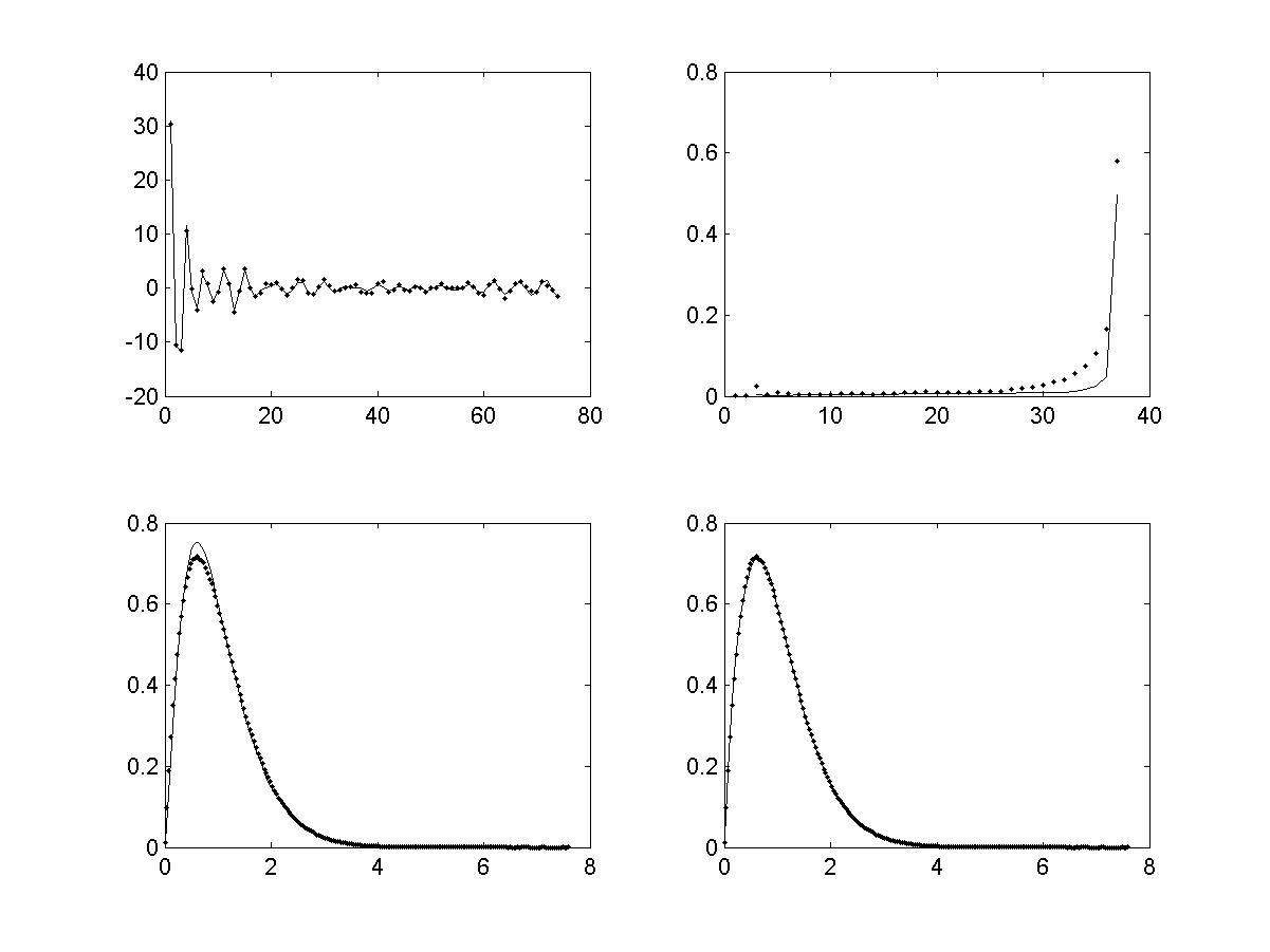
The one term and ten terms approximations of the density were then computed and compared with the empirical density of ${\bf R}_{kk}^{2}$ for $k=1,\dots,p$. The results are given in fig.1. In the top left part the real part of the signal and of the data are plotted. In the top right part the $L_{2}$ norm of the difference between the empirical density of ${\bf R}_{kk}^{2},k=1,\dots,p$ computed by MonteCarlo simulation and its approximation obtained by truncating the series expansion of the density after the first term and after the first $10$ terms is given. In the bottom left part the density of ${\bf R}_{kk}^{2},\;k=36,$ approximated by the first term of its series expansion and the empirical density are plotted. In the bottom right part the density of ${\bf R}_{kk}^{2},\;k=36,$ approximated by the first $10$ terms of its series expansion and the empirical density are plotted. It can be noticed that the first order approximation is quite good even if it become worse for large $k$. The choice $\sigma=0.5$ is justified by the fact that this value is in the range of values used in the examples below. However the same kind of conclusions can be drawn for every SNR .

To appreciate the advantage of the closed form estimate $\hat{h}(z)$ with respect to an estimate of the condensed density obtained by MonteCarlo simulation an experiment was performed. $N=100$ independent realizations of the r.v. generated above were considered. We notice that the frequencies of the $3^{rd}$ and $4^{th}$ components are closer than the Nyquist frequency ($0.21-0.20=0.01<1/n=0.0135$). Hence a super-resolution problem is involved in this case. Two values of the noise s.d. $\sigma$ were used

$$\sigma=0.2,\;0.8.$$

An estimate of $h(z)$ was computed on a square lattice of dimension $m=100$ by

$$\hat{h}(z)\propto\sum_{r=1}^{N}\sum_{k=1}^{p}\hat{\Delta}\left\{\Psi\left[\left(\frac{R_{kk}^{(r)}(z)^{2}}{\sigma^{2}\beta}+1\right)\right]\right\}$$

where R(r)​(z)superscriptπ‘…π‘Ÿπ‘§R^{(r)}(z) 
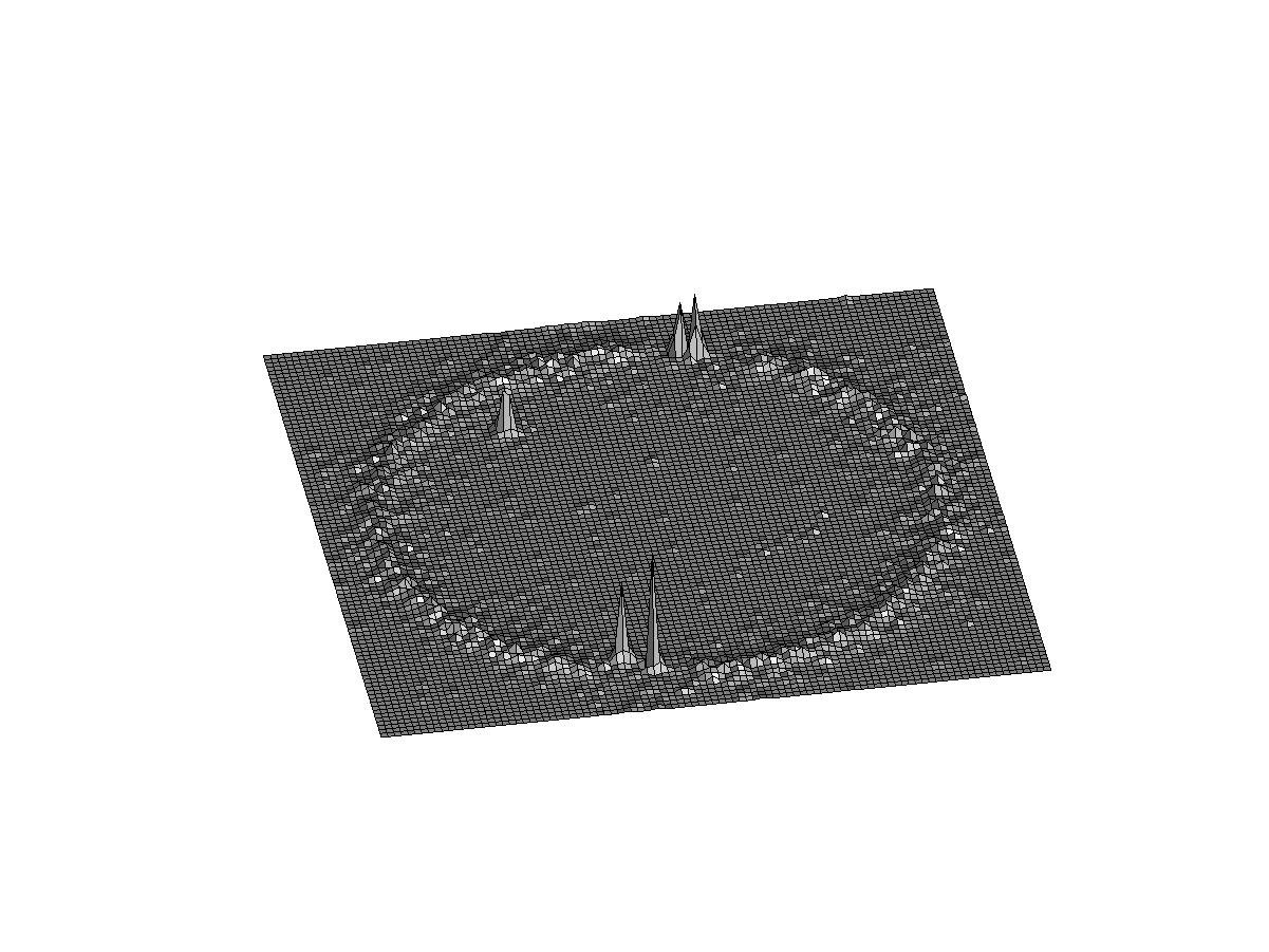
is obtained by the QR factorization of the matrix U1(r)βˆ’z​U0(r).superscriptsubscriptπ‘ˆ1π‘Ÿπ‘§superscriptsubscriptπ‘ˆ0π‘ŸU_{1}^{(r)}-zU_{0}^{(r)}. In the top part of fig.2 the estimate of h​(z)β„Žπ‘§h(z) obtained by Monte Carlo simulation is plotted. In the bottom part the smoothed estimates h^​(z)^β„Žπ‘§\hat{h}(z) for Οƒ=0.2𝜎0.2\sigma=0.2 and Ξ²=5​n𝛽5𝑛\beta=5n based on a single realization was plotted. In
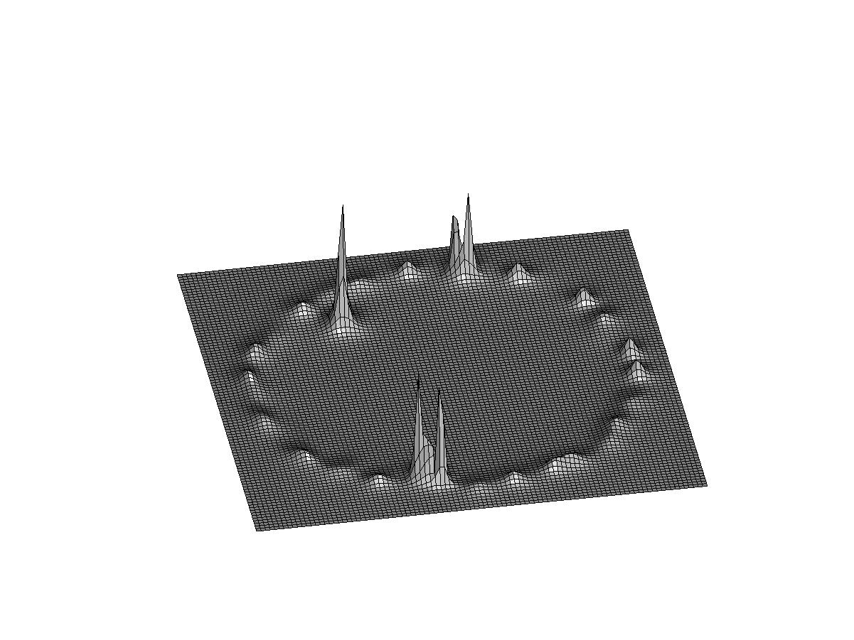
 fig.3 the results obtained with Οƒ=0.8𝜎0.8\sigma=0.8 and Ξ²=5​n𝛽5𝑛\beta=5n are shown. We notice that by the proposed method we get an improved qualitative information with respect to that obtained by replicated measures. This is an important feature for applications where usually only one data set is measured. We also notice that when Οƒ=0.2𝜎0.2\sigma=0.2 the probability to find a root of P​(z)𝑃𝑧P(z) in a neighbor of ΞΎjsubscriptπœ‰π‘—\xi_{j} is larger than the probability to find it elsewhere. This is no longer true when Οƒ=0.8𝜎0.8\sigma=0.8 even if the signal-related complex exponentials are well separated. In the following we will say that the complex exponential model is identifiable if this last case occurs and it is strongly identifiable if the first case occurs. Therefore if the model is identifiable the signal-related complex exponentials are well separated but the relative importance of some of them - measured by the value of the local maxima of h​(z)β„Žπ‘§h(z) - is not larger than the relative importance of some noise-related complex exponentials. Therefore in this case we need some a-priori information about the location of the ΞΎjsubscriptπœ‰π‘—\xi_{j} in order to separate signal-related components from the noise-related ones.

We want now to show by means of a small simulation study the quality of the estimates of the parameters ${p^{*}},\;\underline{\xi}$ and $\underline{c}$ which can be obtained from $\hat{h}(z)$. To this aim the following estimation procedure was used:

  • β€’

    the local maxima of $\hat{h}(z)$ are computed and sorted in decreasing magnitude

  • β€’

    a clustering method is used to group the local maxima into two groups. If the model is strongly identifiable the signal-related maxima are larger than the noise-related ones, therefore a simple thresholding is enough to separate the two groups. A good threshold is the one that produces an estimate of sksubscriptπ‘ π‘˜s_{k} which best fits the data $a_{k}$ in $L_{2}$ norm as the noise is assumed to be Gaussian

  • β€’

    the cardinality $\hat{p}$ of the class with largest average value is an estimate of ${p^{*}}$

  • β€’

    the local maxima $\hat{\xi}_{j},j=1,\dots,\hat{p}$ of the class with largest average value are estimates of $\xi_{j},j=1,\dots,{p^{*}}$. Of course if p^β‰ pβˆ—^𝑝superscript𝑝\hat{p}\neq{p^{*}} some $\xi_{j}$ are not estimated or viceversa some spurious complex exponentials are found

  • β€’

    c¯¯𝑐\underline{c} is estimated by solving the linear least squares problem

    $$\hat{\underline{c}}=argmin_{{\underline{x}}}\|V{\underline{x}}-{\underline{a}}\|_{2}^{2},\;\;{\underline{a}}=[a_{0},\dots,a_{n-1}]^{T}$$

    where $V\in I\!\!\!\!{C}^{n\times\hat{p}}$ is the Vandermonde matrix based on $\hat{\xi}_{j},j=1,\dots,\hat{p}$

The bias, variance and mean squared error (MSE) of each parameter separately were estimated. $N=500$ independent data sets ${\underline{a}}^{(r)}$ of length $n$ were generated by using the model parameters given above and $\sigma=0.2$. For $r=1,\dots,N$ the condensed density estimate $\hat{h}^{(r)}(z)$ was computed on a square lattice of dimension $m=100$. The estimation procedure is then applied to each of the $\hat{h}^{(r)}(z),r=1,\dots,N$ and the corresponding estimates $\hat{\xi}_{j}^{(r)},\hat{c}_{j}^{(r)},j=1,\dots,\hat{p}^{(r)}$ of the unknown parameters were obtained. If the estimate $\hat{p}^{(r)}$ was less than the true value ${p^{*}}$, the corresponding data set ${\underline{a}}^{(r)}$ was discarded.

In Table 2 the bias, variance and MSE of each parameter including ${p^{*}}$ is reported. They were computed by choosing among the $\hat{\xi}_{j}^{(r)},j=1,\dots,\hat{p}^{(r)}\geq{p^{*}}$ the one closest to each $\xi_{k},k=1,\dots,{p^{*}}$ and the corresponding $\hat{c}_{j}^{(r)}$. If more than one $\xi_{k}$ is estimated by the same $\hat{\xi}_{j}^{(r)}$ the $r-$th data set ${\underline{a}}^{(r)}$ was discarded. In the case considered all the data sets were accepted.

As a second example the reconstruction of a piecewise constant function from noisy Fourier coefficients is considered. The problem is stated as follows. Given a real interval $[-\pi,\pi]$ and $N+1$ numbers $-\pi\leq l_{1}<l_{2}\dots<l_{N+1}\leq\pi$, let $\mathcal{F}$ be the class of functions defined as

$$F(t)=\sum_{j=1}^{N}w_{j}\chi_{j}(t)\ ,$$

where

$$\chi_{j}(t)=\left\{\begin{array}[]{ll}1&\mbox{if $t\in[l_{j},l_{j+1}]$}\\ 0&\mbox{otherwise}\end{array}\right.\ ,$$

and the $w_{j}$ are real weights. The problem consists in reconstructing a function $F(t)\in\mathcal{F}$ from a finite number of its noisy Fourier coefficients

𝐚k=12β€‹βˆ«βˆ’Ο€Ο€F​(t)​ei​t​k​𝑑t+Ο΅k=sk+Ο΅k,k=0,…,nβˆ’1,formulae-sequencesubscriptπšπ‘˜12superscriptsubscriptπœ‹πœ‹πΉπ‘‘superscriptπ‘’π‘–π‘‘π‘˜differential-d𝑑subscriptbold-italic-Ο΅π‘˜subscriptπ‘ π‘˜subscriptbold-italic-Ο΅π‘˜π‘˜0…𝑛1{\bf a}_{k}=\frac{1}{2}\int_{-\pi}^{\pi}F(t)e^{itk}dt+{\mbox{\boldmath$\epsilon$}}_{k}=s_{k}+{\mbox{\boldmath$\epsilon$}}_{k}\ ,\quad k=0,\dots,n-1\ ,

where ${{\mbox{\boldmath$\epsilon$}}_{k}}$ is a complex Gaussian, zero mean, white noise, with variance $\sigma^{2}$. We are looking for a solution which is not affected by Gibbs artifact and can cope, stably, with the noise. The basic observation is the following. The unperturbed moments sksubscriptπ‘ π‘˜s_{k} are given by

sk=12β€‹βˆ«βˆ’Ο€Ο€F​(t)​ei​t​k​𝑑t=βˆ‘j=1Nwj​sin⁑(Ξ²j​k)k​exp⁑(i​λj​k),subscriptπ‘ π‘˜12superscriptsubscriptπœ‹πœ‹πΉπ‘‘superscriptπ‘’π‘–π‘‘π‘˜differential-d𝑑superscriptsubscript𝑗1𝑁subscript𝑀𝑗subscriptπ›½π‘—π‘˜π‘˜π‘–subscriptπœ†π‘—π‘˜s_{k}=\frac{1}{2}\int_{-\pi}^{\pi}F(t)e^{itk}dt=\sum_{j=1}^{N}w_{j}\frac{\sin(\beta_{j}k)}{k}\exp(i\lambda_{j}k),

where

$\displaystyle\beta_{j}=\frac{l_{j+1}-l_{j}}{2},\;\;\lambda_{j}=\frac{l_{j+1}+l_{j}}{2}.$

Then consider the $Z$-transform of the sequence {sk}subscriptπ‘ π‘˜\{s_{k}\}

$$s(z)=\sum_{j=1}^{N}w_{j}\left(\beta_{j}+\frac{1}{2i}\ln\frac{z-e^{il_{j}}}{z-e^{il_{j+1}}}\right)$$

which converges if $|z|>1$ and is defined by analytic continuation if $|z|\leq 1$. We notice that $s(z)$ has a branch point at $\xi_{j}=e^{il_{j}},j=1,\dots,N+1$ where $l_{j}$ are the

discontinuity points of $F(t)$. It was proved in [17, 18] that the $c_{j}$ are strong attractors of the poles of the Pade’ approximants $[q,r]_{f}(z)$ to the noisy $Z$-transform

$$f(z)=\sum_{k=0}^{\infty}a_{k}z^{-k}$$

when $q,r\rightarrow\infty$ and $q/r\rightarrow 1$. It is easy to show that the poles of $[q,r]_{f}(z)$ are the generalized eigenvalues of the pencil $(U_{1},U_{0})$ built from the data $a_{k},k=0,\dots,{n-1}$ whose condensed density is $h(z)$. Therefore, as shown in [17, 18] the local maxima of $h(z)$ are concentrated along a set of arcs which ends in the branch points $\xi_{j}$ and on a set of arcs close to the unit circle. As the branch points are strong attractors for the Pade’ poles, the probability to find a pole in a neighbor of a branch point is larger than elsewhere, therefore it can be expected that the branch points correspond to the largest local maxima of $h(z)$, as far as the SNR is sufficiently large. In order to compute estimates $\hat{l}_{j}$ of $l_{j}$, it is sufficient to compute the arguments of the main local maxima of $\hat{h}(z)$. The $w_{j}$ are then estimated by taking the median in each interval $[\hat{l}_{j},\hat{l}_{j+1}]$ of the rough estimate of $F(t)$ obtained by taking the discrete Fourier transform of $a_{k},\;k=0,\dots,n-1$. The median is in fact robust with respect to errors affecting $\hat{l}_{j}$.

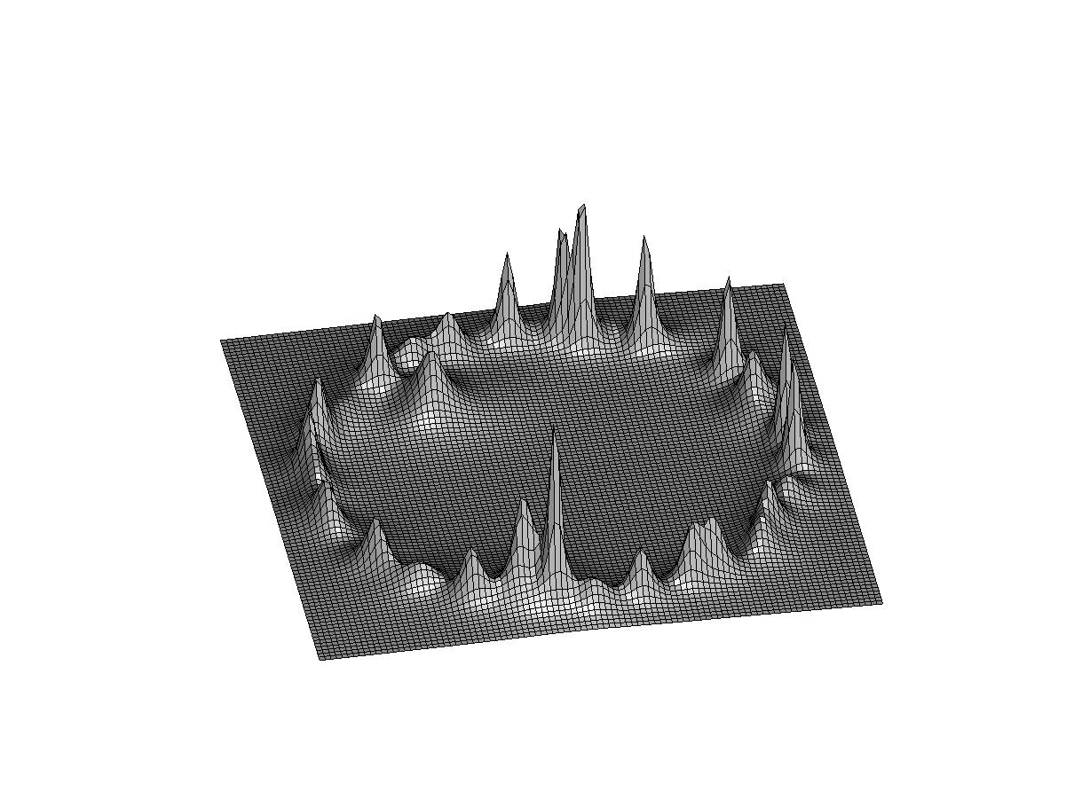
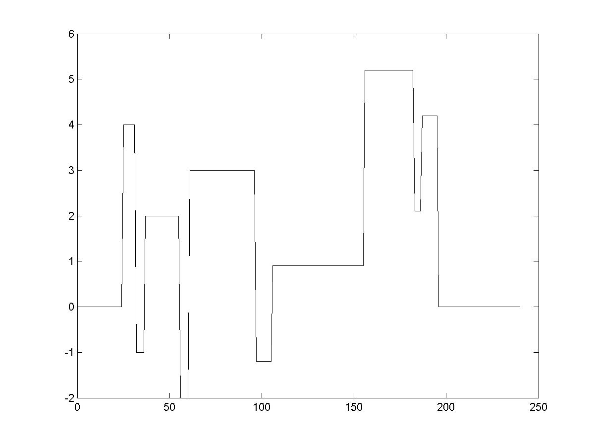
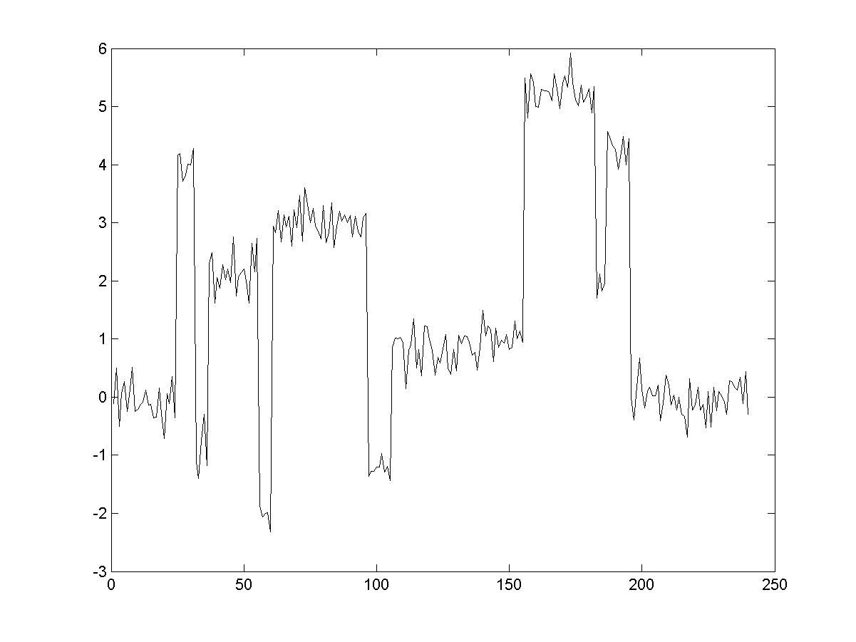
The method was applied to an example considered in [18] where comparisons with other methods were also reported. In the top left part of fig.4 the original function F​(t)𝐹𝑑F(t) is plotted. In the top right the rough estimate of F​(t)𝐹𝑑F(t) when S​N​R=7𝑆𝑁𝑅7SNR=7 is reported where the S​N​R𝑆𝑁𝑅SNR is measured as the ratio of the standard deviations
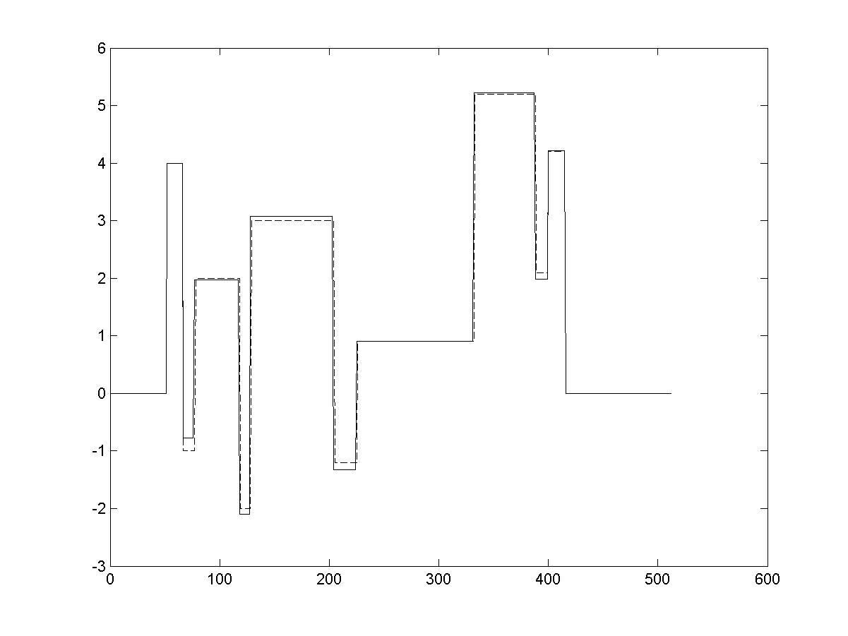
 of {sk}subscriptπ‘ π‘˜\{s_{k}\} and {Ο΅k}subscriptitalic-Ο΅π‘˜\{\epsilon_{k}\}. In the bottom parts the condensed density and the reconstructed function F^​(t)^𝐹𝑑\hat{F}(t) are plotted. Looking at the condensed density we notice that the model is strongly identifiable, therefore the estimation procedure outlined above was 
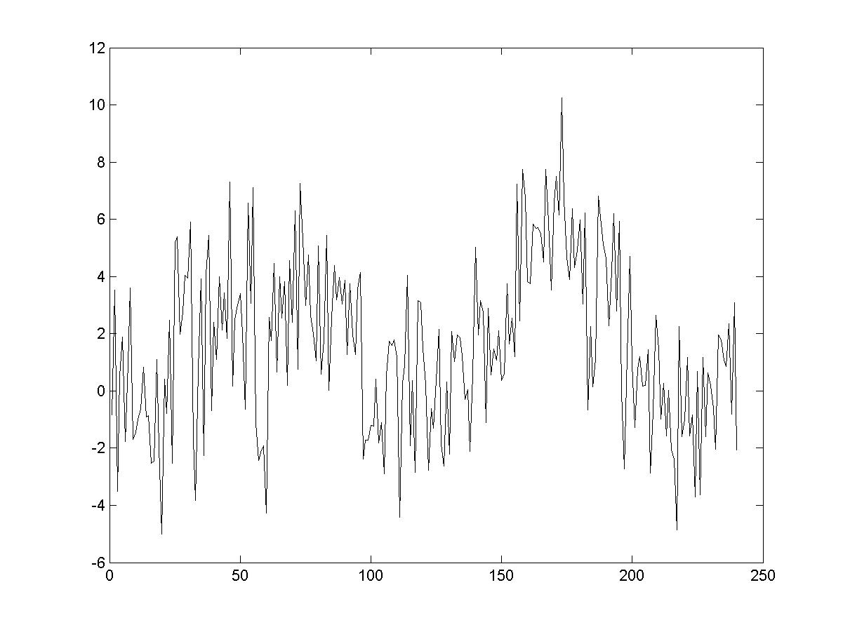
applied. In fig.5 the same quantities as above but with S​N​R=1𝑆𝑁𝑅1SNR=1 are plotted. In this case the model is identifiable but not strongly therefore the clustering step does not work. The number of complex exponentials used to get the reconstruction plotted in fig.5 is p^=20^𝑝20\hat{p}=20 and was found by trial and errors.

We notice that when $SNR=7$ we get an almost perfect reconstruction, better than that reported in [18]. When $SNR=1$ the reconstruction quality is worse as expected but still comparable with the one reported in [18].

References

  • [1] Abate J., Whitt, W. (1999) Infinite series representations of Laplace transforms of probability density functions for numerical inversion, J.Op.Res.Soc.Japan, 42,3 268-285
  • [2] Barone, P. (2010). Estimation of a new stochastic transform for solving the complex exponentials approximation problem: computational aspects and applications, Digital Signal Process., 20,3 724-735
  • [3] Barone, P. (2008). A new transform for solving the noisy complex exponentials approximation problem, J. Approx. Theory 155 1 27.
  • [4] Barone, P. (2005). On the distribution of poles of Pade’ approximants to the Z-transform of complex Gaussian white noise, J. Approx. Theory 132 224-240.
  • [5] Barone, P. (2003). Orthogonal polynomials, random matrices and the numerical inversion of Laplace transform of positive functions. J.Comp. Applied Math. 155, 2 307-330.
  • [6] Barone, P. (2003). Random matrices in Magnetic Resonance signal processing. The 8-th SIAM Conference on Applied Linear Algebra
  • [7] Barone, P., Ramponi, A., Sebastiani, G.(2001). On the numerical inversion of the Laplace transform for Nuclear Magnetic Resonance relaxometry. Inverse Problems 17 77-94.
  • [8] Barone, P., March, R. (2001). A novel class of PadΓ© based method in spectral analysis. J. Comput. Methods Sci. Eng. 1 185-211.
  • [9] Barone, P., March, R. (1998). Some properties of the asymptotic location of poles of PadΓ© approximants to noisy rational functions, relevant for modal analysis. IEEE Trans. Signal Process. 46 2448-2457.
  • [10] Barone, P., Ramponi, A.(2000). A new estimation method in modal analysis. IEEE Trans. Signal Process. 48 1002-1014.
  • [11] Bartlett, M.S.(1933). On the theory of statistical regression. Proc. R. Soc. Edinb. 53 260-283.
  • [12] Deift, P.(2000). Orthogonal polynomials and random matrices: a Riemann-Hilbert approach , American Mathematical Society, Providence, RI.
  • [13] Groetsch, C.W.(1991). Differentiation of approximately specified functions. The American Mathematical Monthly 98,9 847-850.
  • [14] Hammersley, J.M. (1956). The zeros of a random polynomial, Proc. Berkely Symp. Math. Stat. Probability 3rd,2 89-111.
  • [15] Henrici, P. (1977) . Applied and computational complex analysis vol.I, John Wiley and Sons, New York.
  • [16] Johnson, N.L., Kotz, S.(1970). Continuous univariate distributions, vol.2, John Wiley and Sons, New York.
  • [17] March, R., Barone, P.(1998). Application of the PadΓ© method to solve the noisy trigonometric moment problem: some initial results. SIAM J. Appl. Math. 58 324-343.
  • [18] March, R., Barone, P.(2000). Reconstruction of a piecewise constant function from noisy Fourier coefficients by PadΓ© method. SIAM J. Appl. Math. 60 1137-1156.
  • [19] Mathai, A.M., Provost,B.(1977). Quadratic forms in random variables, Marcel Dekker, New York.
  • [20] Sanjel, D., Balakrishnan, N. (2008). A Laguerre polynomial approximation for a goodness-of-fit test for exponential distribution based on progressively censored data, J. Stat. Comput. Simul. 78 503-513.
  • [21] van den Bos, A.(1995). The multivariate complex normal distribution - A generalization, IEEE Trans. Inf. Theory 41,2 537-539.
  • [22] Tziritas G.G.(1987). On the distribution of positive-definite Gaussian quadratic forms, IEEE Trans. Inf. Theory 33,6 895-906.
${p^{*}}$ b​i​a​s​(p^)π‘π‘–π‘Žπ‘ ^𝑝bias(\hat{p}) $s.d.(\hat{p})$ $MSE(\hat{p})$
5 0.0000 0.0000 0.0000
$\xi_{j}$ b​i​a​s​(ΞΎ^j)π‘π‘–π‘Žπ‘ subscript^πœ‰π‘—bias(\hat{\xi}_{j}) $s.d.\hat{\xi}_{j}$ $MSE(\hat{\xi}_{j})$
$j=1$ -0.2796 - 0.8606i -0.0008 + 0.0001i 0.0000 0.0000
$j=2$ -0.1782 - 0.9344i 0.0036 - 0.0010i 0.0000 0.0000
$j=3$ 0.3090 + 0.9510i 0.0057 - 0.0064i 0.0031 0.0001
$j=4$ 0.2487 + 0.9685i -0.0058 + 0.0110 0.0019 0.0002
$j=5$ -0.4354 + 0.5993i -0.0047 + 0.0054i 0.0108 0.0002
$c_{j}$ b​i​a​s​(c^j)π‘π‘–π‘Žπ‘ subscript^𝑐𝑗bias(\hat{c}_{j}) $s.d.(\hat{c}_{j})$ $MSE(\hat{c}_{j})$
$j=1$ 6.0000 0.0440 0.1238 0.0173
$j=2$ 3.0000 -0.0407 0.0688 0.0064
$j=3$ 1.0000 0.0441 0.0736 0.0074
$j=4$ 1.0000 -0.6767 0.0808 0.4644
$j=5$ 20.0000 -0.1007 0.2574 0.0764
Table 2: Statistics of the parameters $\hat{p}$, $\hat{\xi}_{j},j=1,\dots,{p^{*}}$ and $\hat{c}_{j},j=1,\dots,{p^{*}}$
Refer to caption
Figure 1: Top left: real part of the signal (solid) and data (dotted) with $\sigma=0.5$; top right: $L_{2}$ norm of the difference between the empirical density of ${\bf R}_{kk}^{2},k=1,\dots,30$ computed by MonteCarlo simulation with $4\cdot 10^{6}$ samples and its approximation obtained by truncating the series expansion of the density after the first term (dotted) and after the first $10$ terms (solid); bottom left: density of ${\bf R}_{kk}^{2},\;k=36,$ approximated by the first term of its series expansion (solid), empirical density (dotted); bottom right: density of ${\bf R}_{kk}^{2},\;k=36,$ approximated by the first $10$ terms of its series expansion (solid), empirical density (dotted).
Refer to caption
Refer to caption
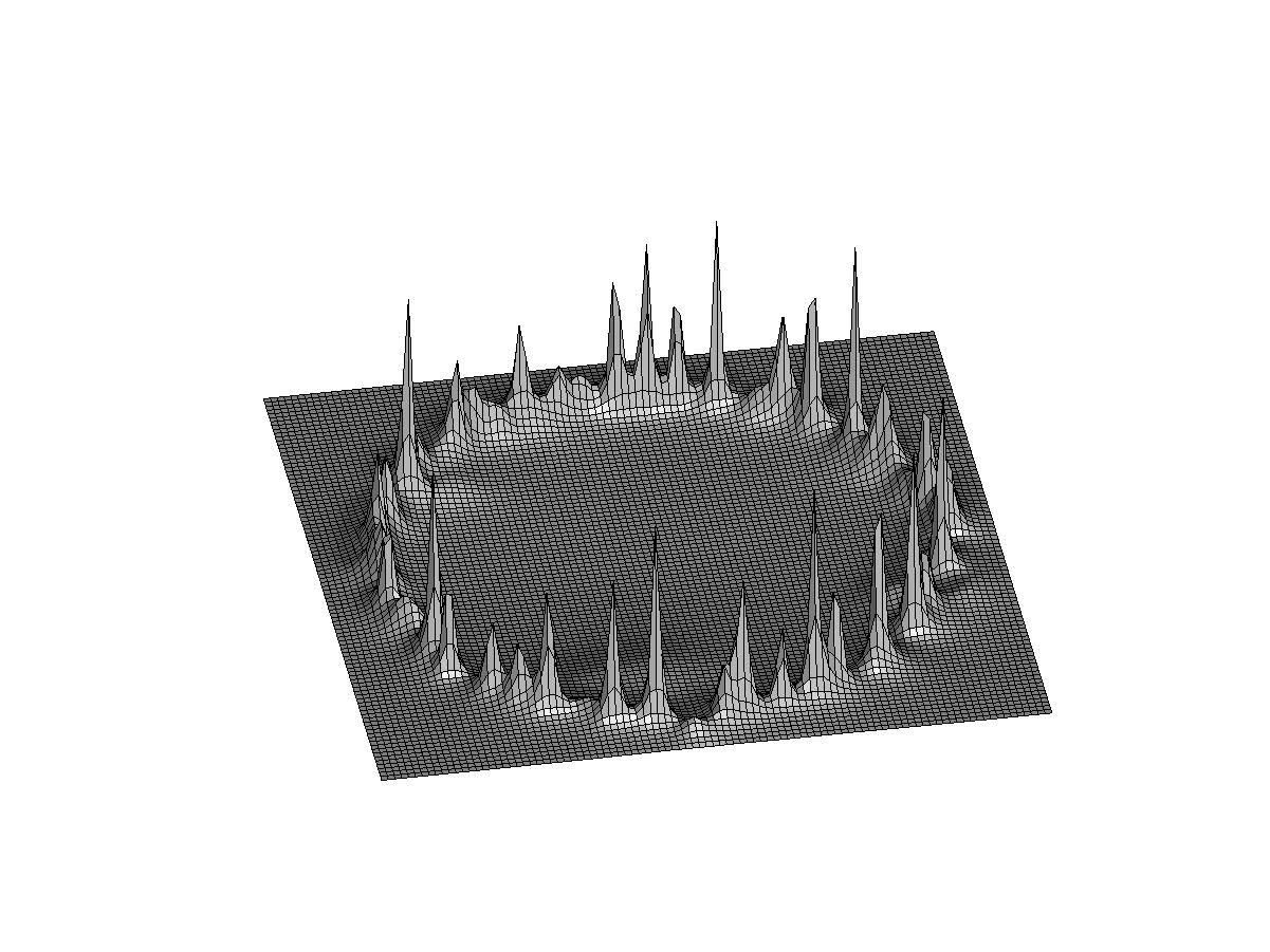
Figure 2: Top: Monte Carlo estimate of the condensed density when $\sigma=0.2$; bottom: estimate of the condensed density by the closed form approximation with $\beta=14.8$.
Refer to caption
Refer to caption
Figure 3: Top: Monte Carlo estimate of the condensed density when $\sigma=0.8$; bottom: estimate of the condensed density by the closed form approximation with $\beta=237$.

Refer to caption Β Β Β Β Β  Refer to caption

Refer to caption Β Β Β Β Β  Refer to caption

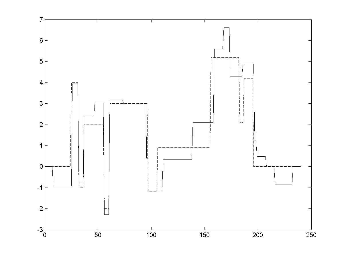
Figure 4: Top left: original function; top right: rough estimate of $F(t)$ when the moments are affected by a Gaussian noise with $SNR=7$. Bottom left: estimate of the condensed density by the closed form approximation; bottom right: reconstruction of the original function.

Refer to caption Β Β Β Β Β Refer to caption

Refer to caption Β Β Β Β Β Refer to caption

Figure 5: Top left: original function; top right: rough estimate of $F(t)$ when the moments are affected by a Gaussian noise with $SNR=1$. Bottom left: estimate of the condensed density by the closed form approximation; bottom right: reconstruction of the original function.