Quantum Oscillations of Tunnel Magnetoresistance Induced by Spin-Wave Excitations in Ferromagnet-Ferromagnet-Ferromagnet Double Barrier Tunnel Junctions

Abstract

The possibility of quantum oscillations of the tunnel conductance and magnetoresistance induced by spin-wave excitations in a ferromagnet-ferromagnet-ferromagnet double barrier tunnel junction, when the magnetizations of the two side ferromagnets are aligned antiparallel to that of the middle ferromagnet, is investigated in a self-consistent manner by means of Keldysh nonequilibrium Green function method. It has been found that owing to the s-d exchange interactions between conduction electrons and the spin density induced by spin accumulation in the middle ferromagnet, the differential conductance and the TMR indeed oscillate with the increase of bias voltage, being consistent with the phenomenon that is observed recently in experiments. The effects of magnon modes, the energy levels of electrons as well as the molecular field in the central ferromagnet on the oscillatory transport property of the system are also discussed.

I Introduction

In past decades, the spin-dependent transport properties in magnetic tunnel junctions (MTJs) have been extensively investigated both experimentally and theoretically, where a great progress has been made (see, e.g. Refs. Prinz ; Wolf ; Zutic ; tserk ; Su for reviews). It has been unveiled that owing to the conduction electron scatterings, the tunnel current through the MTJ is modulated by the relative orientation of magnetizations, giving rise to the so-called tunnel magnetoresistance (TMR) effect. As the quality of tunnel junctions is being improved, a large TMR, which is expected by practical applications, has been achieved in several systems. On the other hand, a reverse effect of TMR, coined as the spin transfer effect Berger ; J.C , has also been proposed, which predicts that the orientation of magnetization of free ferromagnetic layer can be switched by passing a spin-polarized electrical current, and spin waves could also be excited. This latter effect has been confirmed experimentally in a number of systems.

Although single barrier MTJs already show abundant characteristics concerning the spin-dependent electrical transport, a double barrier magnetic tunnel junction (DBMTJ), in which the formation of quantum well states and the resonant tunneling phenomenon are theoretically anticipated, has also attracted much attention in recent years Zhang ; F.M ; Zhang2 ; Sheng ; Stein ; zhu1 ; jin1 ; zhu2 ; Colis ; Han ; jin2 ; zhu3 ; mu1 ; jin3 ; jin4 ; mu2 ; Xing ; Nozaki ; Yan ; Zeng . In order to observe the coherent tunneling thru the DBMTJ, people have attempted to improve the junction quality to eliminate the influences from the interface roughness and impurity scattering, and remarkable advances have been achieved on this aspect.

Recently, an unusual magnetotransport phenomenon in the ferromagnet-ferromagnet-ferromagnet (FM-FM-FM) DBMTJs was reported by Zeng et al. Zeng . They observed that, when the magnetization of center (free) magnetic layer was antiparallel (AP) to the magnetization of the two outer (pinned) magnetic layers, the conductance and TMR oscillate distinctly with the applied bias voltage, while for the parallel (P) situation, no such oscillation was seen. Unlike the previous oscillatory tunnel magnetoresistance, this unusual phenomenon can neither be explained by Coulomb blockade effect since the middle FM layer is continuous, the charge effect should be equal in P and AP configurations and the charging energy is negligibly small, nor be attributed to the resonant tunneling, because the observed period of oscillation is too small to account for the energy level spacing of the quantum well states. Considering that the conductance oscillation is asymmetrical for P and AP configurations, and the energy level of the unusual phenomenon is the same as the typical energy of a magnon, one may speculate that the unusual oscillation behavior could be induced by the magnon-assisted tunneling Zeng . This is because in the AP state, the nonequilibrium spin density, which is proportional to the applied bias, could be accumulated near the interfaces in the middle region to emit spin waves, and the magnon-assisted tunneling would contribute to the conductance, while in the P state the spin wave emission is forbidden due to the spin angular momentum conservation, as discussed previously S.Zhang .

As there is no previous theoretical study devoting to the investigation on the possible quantum oscillations induced by spin wave excitations, in this paper, by using the nonequilibrium Green function method, we shall examine theoretically the above-mentioned idea by studying the possibility of magnon-assisted tunneling in the FM-FM-FM DBMTJ, and explore whether the magnon-assisted tunneling could really cause the oscillations of the differential conductance and TMR with the applied bias voltage.

The rest of this paper is organized as follows: In Sec. II, a model is proposed. The tunnel current and relevant Green functions are obtained in terms of the nonequilibrium Green function technique in Sec. III. In Sec. IV, the transport properties of the system are numerically investigated, and some discussions are presented. Finally, a brief summary is given in Sec. V.

II Model

Let us consider a FM-FM-FM DBMTJ with three FM layers separated by two thin insulating films. Suppose that the left (L) and right (R) FM electrodes with magnetizations aligned parallel are applied by bias voltages $-V/2$ and $V/2$, respectively. The magnetization of the middle FM layer is presumed to be antiparallel to those of the L and R electrodes so that spin waves can be emitted in the middle FM layer because of spin accumulation. The schematic layout of this system is depicted in the inset of Fig. 1(a). The Hamiltonian of the system reads

$$H=H_{L}+H_{R}+H_{C}+H_{LC}+H_{CR},$$ (1)

with

$$H_{\alpha}=\sum_{k_{\alpha}\sigma}\varepsilon_{k_{\alpha}\sigma}a_{k_{\alpha}\sigma}^{+}a_{k_{\alpha}\sigma},\text{ }(\alpha=L,R)$$ (2)

$$H_{C}=\underset{k\sigma}{\sum}\varepsilon_{k\sigma}c_{k\sigma}^{+}c_{k\sigma}+\underset{q}{\sum}\hbar\omega_{q}b_{q}^{+}b_{q},$$ (3)

$$H_{LC} = \underset{k_{L}k\sigma}{\sum}T_{k_{L}k}^{d}(a_{k_{L}\sigma}^{+}c_{k\sigma}+h.c.)$$ (4)

$$+\frac{1}{\sqrt{N}}\underset{k_{L}kq}{\sum}T_{k_{L}kq}^{J}S(q)(a_{k_{L}\uparrow}^{+}c_{k\uparrow}-a_{k_{L}\downarrow}^{+}c_{k\downarrow}+c_{k\uparrow}^{+}a_{k_{L}\uparrow}-c_{k\downarrow}^{+}a_{k_{L}\downarrow})$$

$$+\frac{1}{\sqrt{N}}\underset{k_{L}kq}{\sum}T_{k_{L}kq}^{J}\sqrt{2S}(a_{k_{L}\uparrow}^{+}c_{k\downarrow}b_{q}^{+}+c_{k\uparrow}^{+}a_{k_{L}\downarrow}b_{q}^{+}+a_{k_{L}\downarrow}^{+}c_{k\uparrow}b_{q}+c_{k\downarrow}^{+}a_{k_{L}\uparrow}b_{q}),$$

$$H_{CR} = \underset{k_{R}k\sigma}{\sum}T_{k_{R}k}^{d}(a_{k_{R}\sigma}^{+}c_{k\sigma}+h.c.)$$ (5)

$$+\frac{1}{\sqrt{N}}\underset{k_{R}kq}{\sum}T_{k_{R}kq}^{J}S(q)(a_{k_{R}\uparrow}^{+}c_{k\uparrow}-a_{k_{R}\downarrow}^{+}c_{k\downarrow}+c_{k\uparrow}^{+}a_{k_{R}\uparrow}-c_{k\downarrow}^{+}a_{k_{R}\downarrow})$$

$$+\frac{1}{\sqrt{N}}\underset{k_{R}kq}{\sum}T_{k_{R}kq}^{J}\sqrt{2S}(a_{k_{R}\uparrow}^{+}c_{k\downarrow}b_{q}^{+}+c_{k\uparrow}^{+}a_{k_{R}\downarrow}b_{q}^{+}+a_{k_{R}\downarrow}^{+}c_{k\uparrow}b_{q}+c_{k\downarrow}^{+}a_{k_{R}\uparrow}b_{q}),$$

where $a_{k_{\alpha}\sigma}$ and $c_{k\sigma}$ are annihilation operators of electrons with momentum $k$ and spin $\sigma$ in the $\alpha$ electrode and in the middle FM layer, respectively, $\varepsilon_{k_{\alpha}\sigma}=\varepsilon_{k_{\alpha}}-\sigma{}M_{\alpha}-eV_{\alpha}$ with $\varepsilon_{k_{\alpha}}$ the single-electron energy and $M_{\alpha}$ the molecular field in the $\alpha$ electrode, $\varepsilon_{k\sigma}=\varepsilon_{k}-\sigma M$ with $\varepsilon_{k}$ the single-electron energy and $M$ the molecular field in the middle FM layer, $b_{q}$ is the annihilation operator of magnon with momentum $q$ in the middle region, $\hbar\omega_{q}$ is the magnon energy, $N=\underset{q}{\sum}\langle n_{q}^{s}\rangle$ with $n_{q}^{s}=b_{q}^{+}b_{q}$ is the number of magnons, $S(q)=S-n_{q}^{s}$ where $S=1/2$ is the spin of electron, ${T_{k_{\alpha}k}^{d}}$ are tunneling matrix elements of electrons between the $\alpha$ electrode and middle FM layer, $T_{k_{\alpha}kq}^{J}$ are coupling matrix elements between the electrons in $\alpha$ electrode and magnons in the middle FM region.

It is noting that $H_{LC}$ ($H_{CR}$) describes the coupling between electrons in the L (R) electrode and electrons as well as magnons in the central FM region, where the terms containing $T_{k_{\alpha}kq}^{J}$ in Eqs. (4) and (5) are due to the s-d exchange interactionsS.Zhang . Without loss of generality, we further assume $T_{k_{L}kq}^{J}=\gamma{T_{k_{L}k}^{d}}$ in the following discussions.

III Tunnel Current and Green Functions

III.1 Tunnel Current

Starting from Eq. (1), after some cubersome but straightforward calculations, one may obtain the tunnel electrical current $I$

$$I=I_{L\uparrow}+I_{L_{\downarrow}},$$ (6)

$$I_{L\uparrow}(t) = \frac{2e}{\hbar}\Re e[\sum_{k_{L}k}T_{k_{L}k}^{d}G_{k\uparrow k_{L}\uparrow}^{<}(t,t)+\frac{1}{\sqrt{N}}\underset{k_{L}kq}{\sum}T_{k_{L}kq}^{J}(S-\langle n_{q}^{s}\rangle)G_{k\uparrow k_{L}\uparrow}^{<}(t,t)$$

$$+\sqrt{\frac{2S}{N}}\underset{k_{L}kq}{\sum}T_{k_{L}kq}^{J}G_{k\downarrow k_{L}\uparrow}^{q<}(t,t)],$$

$$I_{L_{\downarrow}}(t) = \frac{2e}{\hbar}\Re e[\sum_{k_{L}k}T_{k_{L}k}^{d}G_{k\downarrow k_{L}\downarrow}^{<}(t,t)-\frac{1}{\sqrt{N}}\underset{k_{L}kq}{\sum}T_{k_{L}kq}^{J}(S-\langle n_{q}^{s}\rangle)G_{k\downarrow k_{L}\downarrow}^{<}(t,t)$$

$$+\sqrt{\frac{2S}{N}}\underset{k_{L}kq}{\sum}T_{k_{L}kq}^{J}G_{k\uparrow k_{L}\downarrow}^{q<}(t,t)],$$

where the lesser Green functions are defined as

$$G_{k\sigma k_{L}\sigma}^{<}(t,t^{\prime})=i\langle a_{k_{L}\sigma}^{+}(t^{\prime})c_{k\sigma}(t)\rangle,$$ (7)

$$G_{k\downarrow k_{L}\uparrow}^{q<}(t,t^{\prime})=i\langle a_{k_{L}\uparrow}^{+}(t^{\prime})b_{q}^{+}(t^{\prime})c_{k\downarrow}(t)\rangle,$$ (8)

$$G_{k\uparrow k_{L}\downarrow}^{q<}(t,t^{\prime})=i\langle a_{k_{L}\downarrow}^{+}(t^{\prime})b_{q}(t^{\prime})c_{k\uparrow}(t)\rangle.$$ (9)

It should be remarked that in the above derivations, we have made decoupling approximations for the terms containing $n_{q}^{s}$ to simplify the calculations. From these above equations, one may see that to get the tunnel electrical current, the lesser Green functions must be obtained. In the following, we shall employ Keldysh’s nonequilibrium Green function method to get all self-consistent equations to determine the lesser Green functions. As the lesser Green function is closely related to the retarded and advanced Green functions according to Keldysh formalism, the relevant retarded and advanced Green functions of electrons and magnons should be first calculated.

Accordingly, the differential tunnel conductance ($G$) is obtained by $G(V)=dI(V)/dV$, and the TMR can be calculated by $TMR=(1-G_{\uparrow\downarrow}/G_{\uparrow\uparrow})$ where $G_{\uparrow\downarrow}$ ($G_{\uparrow\uparrow}$) is the differential conductance when the magnetizations of the middle FM and the side FM are aligned antiparallel (parallel).

III.2 Green Functions of Electrons

Let us define useful retarded Green functions for electrons as

$$G_{k\sigma k^{\prime}\sigma}^{r}(t,t^{\prime})=-i\theta(t-t^{\prime})\langle\{c_{k\sigma}(t),c_{k^{\prime}\sigma}^{+}(t^{\prime})\}\rangle,$$ (10)

$$G_{k\sigma k_{\alpha}\sigma}^{r}(t,t^{\prime})=-i\theta(t-t^{\prime})\langle\{c_{k\sigma}(t),a_{k_{\alpha}\sigma}^{+}(t^{\prime})\}\rangle,$$ (11)

$$G_{k\uparrow k_{\alpha}\downarrow}^{r(q)}(t,t^{\prime})=-i\theta(t-t^{\prime})\langle\{c_{k\uparrow}(t),a_{k_{\alpha}\downarrow}^{+}(t^{\prime})b_{q}(t^{\prime})\}\rangle,$$ (12)

$$G_{k\uparrow k^{\prime}\downarrow}^{r(q)}(t,t^{\prime})=-i\theta(t-t^{\prime})\langle\{c_{k\uparrow}(t),c_{k^{\prime}\downarrow}^{+}(t^{\prime})b_{q}(t^{\prime})\}\rangle,$$ (13)

$$G_{k\downarrow k_{\alpha}\uparrow}^{r(q)}(t,t^{\prime})=-i\theta(t-t^{\prime})\langle\{c_{k\downarrow}(t),a_{k_{\alpha}\uparrow}^{+}(t^{\prime})b_{q}^{+}(t^{\prime})\}\rangle,$$ (14)

$$G_{k\downarrow k^{\prime}\uparrow}^{r(q)}(t,t^{\prime})=-i\theta(t-t^{\prime})\langle\{c_{k\downarrow}(t),c_{k^{\prime}\uparrow}^{+}(t^{\prime})b_{q}^{+}(t^{\prime})\}\rangle.$$ (15)

In terms of the equation of motion, after a tedious calculation, up to the third-order of Green functions, we get the following equations

$$(\varepsilon-\varepsilon_{k_{\alpha}\uparrow})G_{k\uparrow k_{\alpha}\uparrow}^{r}(\varepsilon) = [T^{d}+\frac{T^{J}}{\sqrt{N}}{\sum_{q}}(S-\langle n_{q}^{s}\rangle)]{\sum_{k^{\prime}}}G_{k\uparrow k^{\prime}\uparrow}^{r}(\varepsilon)$$

$$+\sqrt{\frac{2S}{N}}T^{J}\underset{k^{\prime}q}{\sum}G_{k\uparrow k^{\prime}\downarrow}^{r(q)}(\varepsilon),$$

$$(\varepsilon-\varepsilon_{k^{\prime}\uparrow})G_{k\uparrow k^{\prime}\uparrow}^{r}(\varepsilon) = [T^{d}+\frac{T^{J}}{\sqrt{N}}{\sum_{q}}(S-\langle n_{q}^{s}\rangle)]\sum_{\alpha}\sum_{k_{\alpha}}G_{k\uparrow k_{\alpha}\uparrow}^{r}(\varepsilon)$$

$$+\sqrt{\frac{2S}{N}}T^{J}\underset{\alpha}{\sum}\underset{k_{\alpha}q}{\sum}G_{k\uparrow k_{\alpha}\downarrow}^{r(q)}(\varepsilon),$$

$$(\varepsilon-\varepsilon_{k_{\alpha}\downarrow}+\hbar\omega_{q})G_{k\uparrow k_{\alpha}\downarrow}^{r(q)}(\varepsilon) = [T^{d}-\frac{T^{J}}{\sqrt{N}}\sum_{q^{\prime}}(S-\langle n_{q^{\prime}}^{s}\rangle)+\frac{T^{J}}{\sqrt{N}}\langle n_{k_{\alpha}\downarrow}\rangle]\sum_{k^{\prime}}G_{k\uparrow k^{\prime}\downarrow}^{r(q)}(\varepsilon)$$

$$+\sqrt{\frac{2S}{N}}T^{J}(\langle n_{q}^{s}\rangle+\langle n_{k_{\alpha}\downarrow}\rangle)\sum_{k^{\prime}}G_{k\uparrow k^{\prime}\uparrow}^{r}(\varepsilon),$$

$$(\varepsilon-\varepsilon_{k^{\prime}\downarrow}+\hbar\omega_{q})G_{k\uparrow k^{\prime}\downarrow}^{r(q)}(\varepsilon) = \left\{T^{d}-\frac{T^{J}}{\sqrt{N}}[\sum_{q^{\prime}}(S-\langle n_{q^{\prime}}^{s}\rangle)-\sum_{k^{\prime\prime}}\langle c_{k^{\prime}\downarrow}^{+}c_{k^{\prime\prime}\downarrow}\rangle]\right\}\sum_{\alpha}\sum_{k_{\alpha}}G_{k\uparrow k_{\alpha}\downarrow}^{r(q)}(\varepsilon)$$

$$+\sqrt{\frac{2S}{N}}T^{J}(\langle n_{q}^{s}\rangle+\sum_{k^{\prime\prime}}\langle c_{k^{\prime}\downarrow}^{+}c_{k^{\prime\prime}\downarrow}\rangle)\sum_{\alpha}\sum_{k_{\alpha}}G_{k\uparrow k_{\alpha}\uparrow}^{r}(\varepsilon),$$

$$(\varepsilon-\varepsilon_{k_{\alpha}\downarrow})G_{k\downarrow k_{\alpha}\downarrow}^{r}(\varepsilon) = [T^{d}-\frac{T^{J}}{\sqrt{N}}\sum_{q}(S-\langle n_{q}^{s}\rangle)]\sum_{k^{\prime}}G_{k\downarrow k^{\prime}\downarrow}^{r}(\varepsilon)$$

$$+\sqrt{\frac{2S}{N}}T^{J}\sum_{k^{\prime}q}G_{k\downarrow k^{\prime}\uparrow}^{r(q)}(\varepsilon),$$

$$(\varepsilon-\varepsilon_{k^{\prime}\downarrow})G_{k\downarrow k^{\prime}\downarrow}^{r}(\varepsilon) = [T^{d}-\frac{T^{J}}{\sqrt{N}}\sum_{q}(S-\langle n_{q}^{s}\rangle)]\underset{\alpha}{\sum}\underset{k_{\alpha}}{\sum}G_{k\downarrow k_{\alpha}\downarrow}^{r}(\varepsilon)$$

$$+\sqrt{\frac{2S}{N}}T^{J}\underset{\alpha}{\sum}\underset{k_{\alpha}q}{\sum}G_{k\downarrow k_{\alpha}\uparrow}^{r(q)}(\varepsilon),$$

$$(\varepsilon-\varepsilon_{k_{\alpha}\uparrow}-\hbar\omega_{q})G_{k\downarrow k_{\alpha}\uparrow}^{r(q)}(\varepsilon) = [T^{d}+\frac{T^{J}}{\sqrt{N}}\sum_{q^{\prime}}(S-\langle n_{q^{\prime}}^{s}\rangle)+\frac{T^{J}}{\sqrt{N}}\langle n_{k_{\alpha}\uparrow}\rangle]\sum_{k^{\prime}}G_{k\downarrow k^{\prime}\uparrow}^{r(q)}(\varepsilon)$$

$$+\sqrt{\frac{2S}{N}}T^{J}(\langle n_{q}^{s}\rangle+1-\langle n_{k_{\alpha}\uparrow}\rangle)\sum_{k^{\prime}}G_{k\downarrow k^{\prime}\downarrow}^{r}(\varepsilon),$$

$$(\varepsilon-\varepsilon_{k^{\prime}\uparrow}-\hbar\omega_{q})G_{k\downarrow k^{\prime}\uparrow}^{r}(\varepsilon) = \left\{T^{d}+\frac{T^{J}}{\sqrt{N}}[\sum_{q^{\prime}}(S-\langle n_{q^{\prime}}^{s}\rangle)+\underset{k^{\prime\prime}}{\sum}\langle c_{k^{\prime}\uparrow}^{+}c_{k^{\prime\prime}\uparrow}\rangle]\right\}\underset{\alpha}{\sum}\underset{k_{\alpha}}{\sum}G_{k\downarrow k_{\alpha}\uparrow}^{r(q)}(\varepsilon)$$

$$+\sqrt{\frac{2S}{N}}T^{J}(\langle n_{q}^{s}\rangle+1-\underset{k^{\prime\prime}}{\sum}\langle c_{k^{\prime}\uparrow}^{+}c_{k^{\prime\prime}\uparrow}\rangle)\underset{\alpha}{\sum}\underset{k_{\alpha}}{\sum}G_{k\uparrow k_{\alpha}\uparrow}^{r}(\varepsilon),$$

where we have presumed, for simplicity, the coupling matrix elements $T_{k_{L}k}^{d}$ and $T_{k_{L}kq}^{J}$ independent of momentum by considering that only those electrons near the Fermi surface participate in the transport process, and $n_{k_{\alpha}\sigma}=a_{k_{\alpha}\sigma}^{+}a_{k_{\alpha}\sigma}$.

From these equations, the required Green functions can be obtained self-consistently. On the other hand, the lesser self-energy $\Sigma^{<}$ can be approximated by Ng’s ansatz Ng : $\Sigma^{<}=\Sigma_{0}^{<}(\Sigma_{0}^{r}-\Sigma_{0}^{a})^{-1}(\Sigma^{r}-\Sigma^{a})$, where $\Sigma^{r}-\Sigma^{a}=G^{a-1}-G^{r-1}$, $\Sigma_{0}^{r}$ and $\Sigma_{0}^{<}$ are given by the following equations

$$\left(\begin{array}[]{cc}\Sigma_{0\uparrow\uparrow}^{r}(\varepsilon)&\Sigma_{0\downarrow\uparrow}^{r}(\varepsilon)\\ \Sigma_{0\uparrow\downarrow}^{r}(\varepsilon)&\Sigma_{0\downarrow\downarrow}^{r}(\varepsilon)\end{array}\right)=\left(\begin{array}[]{cc}-\frac{i\Gamma_{L\uparrow}}{2}-\frac{i\Gamma_{R\uparrow}}{2}&0\\ 0&-\frac{i\Gamma_{L\downarrow}}{2}-\frac{i\Gamma_{R\downarrow}}{2}\end{array}\right),$$ (16)

$$\left(\begin{array}[]{cc}\Sigma_{0\uparrow\uparrow}^{<}(\varepsilon)&\Sigma_{0\downarrow\uparrow}^{<}(\varepsilon)\\ \Sigma_{0\uparrow\downarrow}^{<}(\varepsilon)&\Sigma_{0\downarrow\downarrow}^{<}(\varepsilon)\end{array}\right)=\left(\begin{array}[]{cc}i\Gamma_{L\uparrow}f(\varepsilon-\frac{eV}{2})+i\Gamma_{R\uparrow}f(\varepsilon+\frac{eV}{2})&0\\ 0&i\Gamma_{L\downarrow}f(\varepsilon-\frac{eV}{2})+i\Gamma_{R\downarrow}f(\varepsilon+\frac{eV}{2})\end{array}\right),$$

where $\Gamma_{\alpha\sigma}(\varepsilon)$ is the linewidth function defined by $\Gamma_{\alpha\sigma}(\varepsilon)=2\pi\underset{k_{\alpha}}{\sum}\rho_{\sigma}(k_{\alpha})\left|T_{k_{L}k}^{d}\right|^{2}$ with $\rho_{\sigma}(k_{\alpha})$ the density of states of electrons with momentum $k_{\alpha}$ and spin $\sigma$ in the $\alpha$th FM electrode, and $f(\varepsilon)$ is the Fermi distribution function. By means of $G^{<}=G^{r}\Sigma^{<}G^{a}$, the lesser Green functions can be procured.

III.3 Green Functions of Magnons

As the number of magnons, $N$, enters into the formalism, we need to obtain the Green functions of magnons to determine $N$ self-consistently. Define the retarded Green function of magnons as

$$G_{qq}^{r}(t,t^{{}^{\prime}})=-i\theta(t-t^{{}^{\prime}})\langle[b_{q}(t),b_{q}^{+}(t^{{}^{\prime}})]\rangle.$$ (17)

By using the equation of motion, we have

$$(\varepsilon-\hbar\omega_{q})G_{qq}^{r}(\varepsilon) = 1+\sqrt{\frac{2S}{N}}\sum\limits_{\alpha}\underset{k_{\alpha}k}{\sum}T_{k_{\alpha}kq}^{J}[G_{kq}^{r(1)}(\varepsilon)+G_{kq}^{r(2)}(\varepsilon)]$$ (18)

$$+\frac{1}{\sqrt{N}}\sum\limits_{\alpha}\underset{k_{\alpha}k}{\sum}T_{k_{\alpha}kq}^{J}[-G_{kq}^{r(3)}(\varepsilon)+G_{kq}^{r(5)}(\varepsilon)-G_{kq}^{r(4)}(\varepsilon)+G_{kq}^{r(6)}(\varepsilon)],$$

where $G_{kq}^{r(i)}(\varepsilon)$ ($i=1,\cdots,5$) are the Fourier transforms of the Green functions defined as below

$$G_{kq}^{r(1)}(t,t^{\prime}) = -i\theta(t-t^{\prime})\langle[b_{q}(t),a_{k_{\alpha}\downarrow}^{+}(t^{\prime})c_{k\uparrow}(t^{\prime})]\rangle,$$

$$G_{kq}^{r(2)}(t,t^{\prime}) = -i\theta(t-t^{\prime})\langle[b_{q}(t),c_{k\downarrow}^{+}(t^{\prime})a_{k_{\alpha}\uparrow}(t^{\prime})]\rangle,$$

$$G_{kq}^{r(3)}(t,t^{\prime}) = -i\theta(t-t^{\prime})\langle[b_{q}(t),b_{q}^{+}(t^{{}^{\prime}})a_{k_{\alpha}\uparrow}^{+}(t^{{}^{\prime}})c_{k\uparrow}(t^{{}^{\prime}})]\rangle,$$

$$G_{kq}^{r(4)}(t,t^{\prime}) = -i\theta(t-t^{\prime})\langle[b_{q}(t),b_{q}^{+}(t^{{}^{\prime}})c_{k\uparrow}^{+}(t^{{}^{\prime}})a_{k_{\alpha}\uparrow}(t^{{}^{\prime}})]\rangle,$$

$$G_{kq}^{r(5)}(t,t^{\prime}) = -i\theta(t-t^{\prime})\langle[b_{q}(t),b_{q}^{+}(t^{{}^{\prime}})a_{k_{\alpha}\downarrow}^{+}(t^{{}^{\prime}})c_{k\downarrow}(t^{{}^{\prime}})]\rangle,$$

$$G_{kq}^{r(6)}(t,t^{\prime}) = -i\theta(t-t^{\prime})\langle[b_{q}(t),b_{q}^{+}(t^{{}^{\prime}})c_{k\downarrow}^{+}(t^{{}^{\prime}})a_{k_{\alpha}\downarrow}(t^{{}^{\prime}})]\rangle.$$

By using repeatedly the equation of motion, and making appropriate cut-off approximations, up to the second order, we have

$$G_{kq}^{r(1)}(\varepsilon)=-T^{J}\sqrt{\frac{2S}{N}}\frac{\langle n_{k_{\alpha}\downarrow}\rangle-\sum_{k^{\prime}}\langle c_{k^{\prime}\uparrow}^{+}c_{k\uparrow}\rangle}{\varepsilon-\varepsilon_{k_{\alpha}\downarrow}+\varepsilon_{k\uparrow}}G_{qq}^{r}(\varepsilon),$$ (19)

$$G_{kq}^{r(2)}(\varepsilon)=T^{J}\sqrt{\frac{2S}{N}}\frac{\langle n_{k_{\alpha}\uparrow}\rangle-\sum_{k^{\prime}}\langle c_{k\downarrow}^{+}c_{k^{\prime}\downarrow}\rangle}{\varepsilon+\varepsilon_{k_{\alpha}\uparrow}-\varepsilon_{k\downarrow}}G_{qq}^{r}(\varepsilon),$$ (20)

$$G_{kq}^{r(3)}(\varepsilon)=-\{\frac{\frac{T^{J}}{\sqrt{N}}(1-\langle n_{k_{\alpha}\uparrow}\rangle)\sum_{k^{\prime}}\langle c_{k^{\prime}\uparrow}^{+}c_{k\uparrow}\rangle-[T^{d}+\frac{T^{J}}{\sqrt{N}}\sum_{q^{\prime}}(S-\langle n_{q^{\prime}}^{s}\rangle)](\sum_{k^{\prime}}\langle c_{k^{\prime}\uparrow}^{+}c_{k\uparrow}\rangle-\langle n_{k_{\alpha}\uparrow}\rangle)}{\varepsilon-\hbar\omega_{q}-\varepsilon_{k_{\alpha}\uparrow}+\varepsilon_{k\uparrow}}\}G_{qq}^{r}(\varepsilon),$$ (21)

$$G_{kq}^{r(4)}(\varepsilon)=-\{\frac{\frac{T^{J}}{\sqrt{N}}(1-\sum_{k^{\prime}}\langle c_{k\uparrow}^{+}c_{k^{\prime}\uparrow}\rangle)\langle n_{k_{\alpha}\uparrow}\rangle+[T^{d}+\frac{T^{J}}{\sqrt{N}}\sum_{q^{\prime}}(S-\langle n_{q^{\prime}}^{s}\rangle)](\sum_{k^{\prime}}\langle c_{k\uparrow}^{+}c_{k^{\prime}\uparrow}\rangle-\langle n_{k_{\alpha}\uparrow}\rangle)}{\varepsilon-\hbar\omega_{q}+\varepsilon_{k_{\alpha}\uparrow}-\varepsilon_{k\uparrow}}\}G_{qq}^{r}(\varepsilon),$$ (22)

$$G_{kq}^{r(5)}(\varepsilon)=\{\frac{\frac{T^{J}}{\sqrt{N}}(1-\langle n_{k_{\alpha}\downarrow}\rangle)\sum_{k^{\prime}}\langle c_{k^{\prime}\downarrow}^{+}c_{k\downarrow}\rangle+[T^{d}-\frac{T^{J}}{\sqrt{N}}\sum_{q^{\prime}}(S-\langle n_{q^{\prime}}^{s}\rangle)](\sum_{k^{\prime}}\langle c_{k^{\prime}\downarrow}^{+}c_{k\downarrow}\rangle-\langle n_{k_{\alpha}\downarrow}\rangle)}{\varepsilon-\hbar\omega_{q}-\varepsilon_{k_{\alpha}\downarrow}+\varepsilon_{k\downarrow}}\}G_{qq}^{r}(\varepsilon),$$ (23)

$$G_{kq}^{r(6)}(\varepsilon)=\{\frac{\frac{T^{J}}{\sqrt{N}}(1-\sum_{k^{\prime}}\langle c_{k\downarrow}^{+}c_{k^{\prime}\downarrow}\rangle)\langle n_{k_{\alpha}\downarrow}\rangle-[T^{d}-\frac{T^{J}}{\sqrt{N}}\sum_{q^{\prime}}(S-\langle n_{q^{\prime}}^{s}\rangle)](\sum_{k^{\prime}}\langle c_{k\downarrow}^{+}c_{k^{\prime}\downarrow}\rangle-\langle n_{k_{\alpha}\downarrow}\rangle)}{\varepsilon-\hbar\omega_{q}+\varepsilon_{k_{\alpha}\downarrow}-\varepsilon_{k\downarrow}}\}G_{qq}^{r}(\varepsilon).$$ (24)

The number of magnons can thus be obtained by the spectral theorem

$$N=\sum\limits_{q}\langle n_{q}^{s}\rangle=\sum\limits_{q}\Im m\int\frac{d\varepsilon}{2\pi}G_{qq}^{<}(\varepsilon)=\sum\limits_{q}\int\frac{d\varepsilon}{2\pi}f_{s}(\varepsilon)[G_{qq}^{r}(\varepsilon)-G_{qq}^{a}(\varepsilon)],$$ (25)

where $f_{s}(\varepsilon)$ is the Bose distribution function.

To get physical quantities under interest, all above equations should be numerically solved in a self-consistent manner.

IV Results and Discussions

To proceed the numerical calculations, we need to make some assumptions. Since the number of the above self-consistent equations nonlinearly increases with increasing the number of wave vectors of electrons and the number of spin-wave modes in the middle FM region, which makes the calculations too complicated to perform, for the sake of simplicity but without losing the generality, we shall only consider the situations where both the numbers of $k$ and $q$ taken in the following calculations are not so large that the numerical calculations can be readily proceeded. This is plausible, because the magnon-assisted transport property mainly depends on the low-lying quantum well states of electrons in the middle FM, and only the lower modes of spin waves are easy to emitBerger , leading to small energy levels of magnonsZeng . Besides, considering that only those electrons near the Fermi surface participate in the tunneling process, we may take $\varepsilon_{k\sigma}\approx\varepsilon_{k_{F}}-\sigma M$, denoted by $\varepsilon_{\uparrow}$ and $\varepsilon_{\downarrow}$ for spin up and down electrons, respectively. In addition, we suppose that the two side FM electrodes are made of the same materials, i.e., $M_{L}=M_{R}$, $P_{L}=P_{R}=P$, where $P_{L(R)}=[\Gamma_{L(R)\uparrow}-\Gamma_{L(R)\downarrow}]/[\Gamma_{L(R)\uparrow}+\Gamma_{L(R)\downarrow}]$ is the polarization of the left (right) FM layer. Then, the linewidth function can be written as $\Gamma_{L\uparrow,\downarrow}=\Gamma_{R\uparrow,\downarrow}=\Gamma_{0}(1\pm P)$, where $\Gamma_{0}=\Gamma_{L(R)\uparrow}(P=0)=\Gamma_{L(R)\downarrow}(P=0)$ will be taken as an energy scale. In the following, we will take $P=0.7$, $k_{B}T=0.04\Gamma_{0}$, $I_{0}=\frac{e\Gamma_{0}}{\hbar}$ and $G_{0}=\frac{e^{2}}{\hbar}$ will be taken as scales for the tunnel current and the differential conductance, respectively.

IV.1 Effect of Magnon-Assisted Tunneling

In order to study whether the quantum oscillations of the conductance and TMR observed in the FM-FM-FM tunnel junction are induced by spin-wave excitations owing to spin accumulation, let us first examine the bias dependence of the transport properties by considering the effect of magnon-assisted tunneling in the AP state.

For given energy levels of the electrons and magnons in the middle FM region, the bias dependent tunnel current ($I/I_{0}$), the differential conductance ($G/G_{0}$) and $TMR$ for different $\gamma$ $(=T^{J}/T^{d})$ are shown in Fig. 1. It is observed that the tunnel current increases nonliniearly with increasing the bias voltage. The twisted behavior of $I/I_{0}$ for $\gamma\neq 0$, presented in Fig. 1(a), comes from the magnon-assisted tunneling, as no such behaviors are found for $\gamma=0$ in either AP or P state. This can be clearly seen from the bias dependence of the differential conductance, shown in Fig. 1(b), where the peaks and dips appear for appropriate $\gamma$. Correspondingly, the TMR shows oscillating behavior with increasing the bias voltage, as demonstrated in Fig. 1(c). This observation manifests that the quantum oscillations of the conductance and TMR in the FM-FM-FM tunnel junction can be caused by spin-wave excitations, because when we turn off the effect of spin-wave excitations, the oscillating behaviors of $G$ and $TMR$ disappear. Note that the peak in $G/G_{0}$ and one dip and one peak in $TMR$ are from the quantum resonant tunneling of electrons. A larger TMR can be obtained for large $\gamma$, and due to the s-d exchange interactions that could lead to spin-flip scatterings, the TMR can be negative, as presented in Fig. 1(c).

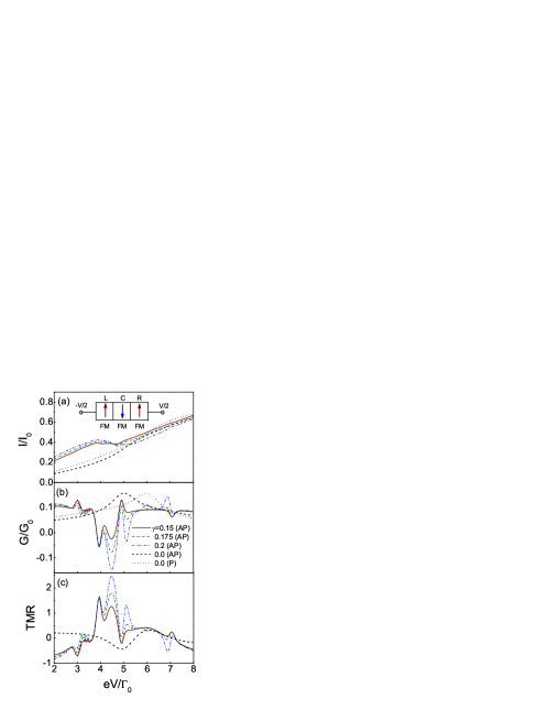
Figure 1: (Color Online) Bias dependence of (a) the tunnel current I, (b) the differential conductance G, and (c) TMR for the different $\gamma$, where $\hbar\omega_{q}=0.5\Gamma_{0}$, $\varepsilon_{\uparrow}=3.0\Gamma_{0}$ and $\varepsilon_{\downarrow}=2.0\Gamma_{0}$.

It should be remarked that the above oscillating behaviors of $G$ and $TMR$ appear only when $\gamma$ is in a suitable range, say, when $\gamma$ is too small, no oscillations can be observed, while $\gamma$ is too large, the self-consistent equations have no solutions.

The reason for the appearance of oscillations is that, when the applied bias voltage exceeds a certain value, the non-equilibrium spin density can be accumulated in the middle FM region, and spin waves can be excited. When polarized electrons from the left FM layer tunnel into the central FM layer, they are subject to scatterings from not only the polarized electrons in the central region but also the spin waves from the accumulation owing to s-d exchange interactions. It is possible that the electrons may turn their spin directions by emission and absorption of magnons, leading to that the tunnel conductance and TMR oscillate under a combination of effects of magnon-assisted tunneling as well as quantum resonant tunnelingmu2 through the quantum well states in the central FM region.

Apparently, the polarized electrical current can excite magnons, while these magnons participate in the tunneling process and in turn influence the tunnel current. The number of magnons must be estimated self-consistently. As an example, in Fig. 2, the bias dependent of the number of magnons $N$ for some parameters is presented. We may see that the number of magnons oscillates with the bias voltage, which could be the main reason for the oscillatory transport property of the system.

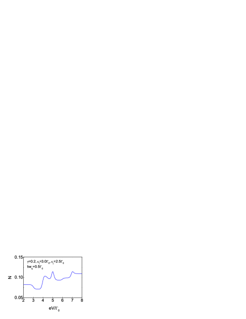
Figure 2: (Color Online) Bias dependence of the number of magnons N in the AP state.

IV.2 Effect of Magnon Modes

There are a number of factors including magnon energy $\hbar\omega_{q}$ that can affect the transport behavior of the FM-FM-FM tunnel junction. The bias dependence of the current, the different conductance and the TMR for different magnon energies is shown in Fig. 3. It can be found that with increasing $\hbar\omega_{q}$, apart from some quantitative changes of peak positions and amplitudes, there are not much qualitative changes of the current, conductance and TMR. Therefore, for a given magnon mode, the magnon energy does not affect qualitatively the transport oscillating behavior of the system. It is noted that, while some positions of the peaks and dips of $G$ and $TMR$ are influenced by the magnon energy, the others are not. This observation indicates that the magnon energy is only one of factors determining the positions and amplitudes of the peaks.

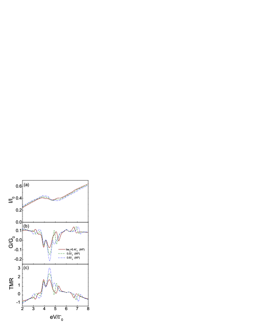
Figure 3: (Color Online) Bias dependence of (a) the tunnel current I, (b) the differential conductance G and (c) TMR for the different $\hbar\omega_{q}$, where $\gamma=0.2$, $\varepsilon_{\uparrow}=3.0\Gamma_{0}$ and $\varepsilon_{\downarrow}=2.0\Gamma_{0}$.

For the sake of simplicity, in the aforementioned analysis we have adopted a single spin-wave mode. Whether are the transport properties of the system much affected qualitatively when we take more spin-wave modes into account? The answer is presented in Fig. 4, where we have taken two and three spin-wave modes to get the tunnel current, differential conductance and TMR. For a comparison, we have also included the case with single mode. One may see that at low biases, the magnon modes do not have so much effect on the behaviors of $I/I_{0}$, $G/G_{0}$ and $TMR$, but at higher voltages the magnitudes of the current, differential conductance as well as TMR change somewhat remarkably. This is because at low biases the spin accumulation effect is small, and the interaction between tunneling electrons and spin-wave modes is weak, leading to the transport properties less influenced; at large biases the spin accumulation effect becomes more pronounced, and the interactions between electrons and magnons are strong, the transport behaviors of the system are thus altered quantitatively. Note that the round peaks and dips in the curves of the tunnel current shown in Fig. 4 may come from combinations of the magnon-assisted tunneling as well as the quantum resonant tunneling.

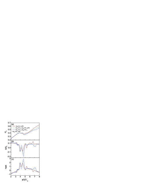
Figure 4: (Color Online) Bias dependence of (a) the tunnel current I, (b) the differential conductance G, and (c) TMR for different spin-wave modes, where $\gamma=0.2$, $\varepsilon_{\uparrow}=3.0\Gamma_{0}$ and $\varepsilon_{\downarrow}=2.0\Gamma_{0}$.

IV.3 Effect of Electron Level in the Middle FM Layer

The bias dependence of the current, the differential conductance and the TMR for different energy levels ($\varepsilon_{{}_{k_{F}}}\equiv\varepsilon$) of the electrons in the middle FM region is given in Fig. 5. It can be observed that with lifting the energy levels of electrons in the central FM layer, the peak and dip positions of $I/I_{0}$, $G/G_{0}$ and $TMR$ change dramatically with increasing the bias voltage, while the shapes of the curves retain quite similar for different energy levels of electrons in the central region. This signifies that the energy levels of electrons in the middle FM region do not affect the oscillating behavior itself of the transport properties, but affect the positions of oscillating peaks and dips. This can be understandable, because the transport behavior of electrons are mainly determined by the scatterings from polarized electrons and magnons to that the electrons are subject, when the energy levels of electrons in the middle region are promoted, the resonant energies in magnon-assisted and quantum resonant tunneling processes become different, resulting in the behaviors shown in Fig. 5.

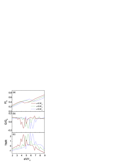
Figure 5: (Color Online) Bias dependence of (a) the tunnel current I, (b) the differential conductance G, and (c) TMR in the AP state for different energy levels of electrons in the middle FM region, where $\gamma=0.2$, $\hbar\omega_{q}=0.5\Gamma_{0}$ and $M=1.0\Gamma_{0}$.

IV.4 Effect of Molecular Field in the Middle FM Layer

The molecular fields of the middle FM layer could also have effect on the transport properties of the system. The bias dependence of the current, differential conductance and TMR for different molecular fields of the central FM region is shown in Fig. 6. It is seen that as the molecular field increases, the magnitude of the tunnel current becomes smaller, and the oscillations of the differential conductance as well as TMR become more apparent, where not only the number but also the positions of the oscillating peaks change with increasing the molecular fields. This fact suggests that the level spacing between the majorty and minority subbands of electrons in the central region plays an important role in the oscillating behaviors of the differential conductance and TMR in the present system.

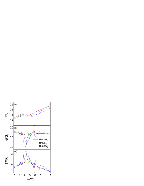
Figure 6: (Color Online) Bias dependence of (a) the tunnel current I, (b) the differential conductance G, and (c) TMR for different molecular fields of the middle FM layer, where $\gamma=0.2$, $\varepsilon=2.5\Gamma_{0}$ and $\hbar\omega_{q}=0.5\Gamma_{0}$.

V Summary

In summary, we have probed the possibility of quantum oscillations of the differential conductance and TMR in the FM-FM-FM tunnel junction in the AP state. By self-consistently taking the s-d exchange interactions between conduction electrons and the nonequilibrium spin density induced by spin accumulation in the middle FM layer into account, we have found that the differential conductance and TMR indeed oscillate with increasing the bias voltage, thereby theoretically confirming qualitatively the inferrer and experimental results presented in Ref. Zeng . It has been unveiled that the average number of magnons oscillates with the bias, which could be the main reason for the oscillations of the conductance and TMR of the system. When we turn off the s-d exchange interactions, i.e., taking $\gamma=0$, no oscillations of the conductance and TMR were observed, showing that the oscilations are indeed caused by the spin-wave excitations induced by spin accumulations. In the P state, owing to the absence of spin accumulationjin3 ; jin4 , no oscillations of the conductance and TMR with the bias can be found. We have also investigated the effects of the magnon modes, the energy levels of electrons as well as the molecular field in the middle FM region, and found that in spite of changes of the positions and amplitudes of the oscillating peaks and dips, the oscillatory behavior of the transport properties is not qualitatively affected. We anticipate that our findings could offer clues for better understanding the experimental observation presented in Ref. Zeng .

Finally, we would like to remark that our preceding discussions could be applicable to the system with a magnetic quantum dot coupled to two ferromagnetic electrodes, where the oscillatory behavior of the transport properties with the bias would be expected if the spin accumulation effect is not neglected. The work toward this direction is under progress.

References

• (1) G. A. Prinz, Science 282, 1660 (1998).
• (2) S. A. Wolf, D. D. Awschalom, R. A. Buhrman, J. M. Daughton, S. von Molnár, M. L. Roukes, A. Y. Chtchelkanova, and D. M. Treger, Science 294, 1488 (2001)
• (3) I. Žutić, J. Fabian and S. D. Sarma, Rev. Mod. Phys. 76, 323 (2004).
• (4) Y. Tserkovnyak, A. Brataas, G.E.W. Bauer, B.I. Halperin, Rev. Mod. Phys. 77, 1375 (2005).
• (5) G. Su, in Progress in Ferromagnetism Research, edited by V. N. Murray (Nova Science Publishers, Inc., New York, 2006), pp. 85-123.
• (6) L. Berger, Phys. Rev. B 54, 9353 (1996).
• (7) J. C. Slonczewski, J. Magn. Magn. Mater. 159, L1 (1996).
• (8) X. Zhang, B. Z. Li, G. Sun, and F. C. Pu, Phys. Rev. B 56, 5484 (1997).
• (9) F. Montaigne, J. Nassar, A. Vaurés, F. Nguyen Van Dau, F. Petroff, A. Schuhl, and A. Fert, Appl. Phys. Lett 73, 2829 (1997).
• (10) X. Zhang, B. Z. Li, G. Sun, and F. C. Pu, Phys. Lett. A 245, 133 (1998).
• (11) L. Sheng, Y. Chen, H. Y. Teng, and C. S. Ting, Phys. Rev. B 59, 480 (1999).
• (12) S. Stein, R. Schmitz, and H. Kohlstedt, Solid State Commum 117, 599 (2001).
• (13) Z. G. Zhu, G. Su, B. Jin and Q. R. Zheng, Inter. J. Mod. Phys. B 16, 2857 (2002).
• (14) B. Jin, G. Su, Q. R. Zheng and M. Suzuki, Phys. Rev. B 68, 144504 (2003).
• (15) Z.G. Zhu, G. Su, Q. R. Zheng and B. Jin, Phys. Rev. B 68, 224413 (2003).
• (16) S. Colis, G. Gieres, L. Bar, and J. Wecker, Appl. Phys. Lett. 83, 948 (2003).
• (17) X. F. Han, S. F. Zhao, F. F. Li, T. Daibou, H. Kubota, Y. Ando, and T. Miyazaki, J. Magn. Magn. Mater. 282, 225 (2004).
• (18) B. Jin, G. Su and Q. R. Zheng, J. Appl. Phys. 96, 5654 (2004).
• (19) Z. G. Zhu, G. Su, Q. R. Zheng and B. Jin, Phys. Rev. B 70, 174403 (2004).
• (20) H. F. Mu, G. Su, Q. R. Zheng and B. Jin, Phys. Rev. B 71, 064412 (2005).
• (21) B. Jin, G. Su and Q. R. Zheng, Phys. Rev. B 71, 144514 (2005).
• (22) B. Jin, G. Su and Q. R. Zheng, Phys. Rev. B 73, 064518 (2006).
• (23) H. F. Mu, G. Su, and Q. R. Zheng, Phys. Rev. B 73, 054414 (2006).
• (24) Z. P. Niu, Z. B. Feng, J. Yang, and D. Y. Xing, Phys. Rev. B 73, 014432 (2006).
• (25) T. Nozaki, N. Tezuka, and K. Inomata Phys. Rev. Lett. 96, 027208 (2006).
• (26) Y. Wang, Z. Y. Lu, X. -G. Zhang, and X. F. Han, Phys. Rev. Lett. 97, 087210 (2006).
• (27) Z. M. Zeng, X. F. Han, W. S. Zhan, Y. Wang, Z. Zhang, and Shufeng Zhang, Phys. Rev. B 72, 054419 (2005).
• (28) S. Zhang, and P. M. Levy , Phys. Rev. Lett. 79, 3744 (1997).
• (29) T. K. Ng, Phys. Rev. Lett. 89, 286803 (2002).
• (30) H. Haug and A. P. Jauho, Quantum Kinetics in Transport and Optics of Semiconductors (Springer, Berlin, 1998), p.166.