Hipparcos distance estimates of the Ophiuchus and the Lupus cloud complexes

We combine extinction maps from the Two Micron All Sky Survey (2MASS) with Hipparcos and Tycho parallaxes to obtain reliable and high-precision estimates of the distance to the Ophiuchus and Lupus dark complexes. Our analysis, based on a rigorous maximum-likelihood approach, shows that the $\rho$-Ophiuchi cloud is located at $(119\pm 6)\mbox{ pc}$ and the Lupus complex is located at $(155\pm 8)\mbox{ pc}$; in addition, we are able to put constraints on the thickness of the clouds and on their orientation on the sky (both these effects are not included in the error estimate quoted above). For Ophiuchus, we find some evidence that the streamers are closer to us than the core. The method applied in this paper is currently limited to nearby molecular clouds, but it will find many natural applications in the GAIA-era, when it will be possible to pin down the distance and three-dimensional structure of virtually every molecular cloud in the Galaxy.

1 Introduction

In recent years, much effort has been dedicated to the study of dark molecular clouds and their dense cores. One of the main motivations for these investigations is the study of the process of star and planet formation in its entirety, and a deeper understanding of the effects of the local environment. A key aspect of the scientific analysis of a dark molecular cloud is its distance, which is related to many physically relevant properties (in particular, the mass scales as the square of the distance). Unfortunately, the distance estimates for many clouds are often plagued by very large uncertainties and it is not rare to see in the literature measurements that differ by large factors. Often, this quantity is inferred by associating the cloud to other astronomical objects whose distance is well known. For example, the Lupus complex is located near the Sco OB2 association (Humphreys, 1978; de Zeeuw et al., 1999), whose distance is estimated to be $\sim 150\mbox{ pc}$ based on the photometry of OB stars (Krauuter, 1991). However, this method is based on some degree of arbitrariness when making the link between the cloud and the other objects, and thus the deduced distance can be completely unreliable.

The cloud complexes considered in this paper, the $\rho$ Ophiuchi and the Lupus dark clouds, are good examples of how different distance estimates made by different authors can be. Quoted values for the $\rho$-Ophiuchi cloud are in the range $120$–$165\mbox{ pc}$, as recently summarized by Rebull et al. (2004). Chini (1981) estimated the distance to be $\sim 160\mbox{ pc}$ from multi-color photometry of heavily absorbed stars in the $\rho$ Oph core, while Knude & Hog (1998) suggested a significantly smaller figure, $\sim 120\mbox{ pc}$. For Lupus, the situation is even more extreme, with estimates from $100\mbox{ pc}$ (Knude & Hog, 1998) to $190\mbox{ pc}$ (Wichmann et al., 1998), both based on Hipparcos data; the most widely accepted distance is in the middle of these two extremes, at approximately $140\mbox{ pc}$ (Hughes et al., 1993; de Zeeuw et al., 1999).

These uncertainties severely hamper our understanding of the physical properties of molecular clouds, and thus our knowledge of star formation. For example, an error by a factor two on the distance of a cloud translates into an error by a factor four in the mass, and has a thus a huge impact on the estimate of the density, size, stability, and star formation efficiency of their cloud cores (see Alves et al., 2007 for further discussions on this point).

In this paper we present accurate distance measurements of the Ophiuchus and Lupus complexes based upon Hipparcos and Tycho parallaxes. Our technique is statistically sound and, when applied to nearby giant molecular clouds, is able to provide accurate distance measurements and related errors. The paper is organized as follows. In Sect. 2 we present the main datasets used and discuss a simple approach to the problem. A more quantitative technique is developed in Sect. 3, where we also presents the results obtained for the two clouds considered in this paper. The technique is further developed in Sect. 4 to include the effects of the cloud thickness and orientation. Finally, in Sect. 5 we briefly discuss the results obtained.

2 Basic analysis

Figure 1: The Ophiuchus region considered. The gray map shows 2MASS/Nicer extinction, with overlaid the $A_{K}=0.1\mbox{ mag}$ (smoothed) contour. The dots indicate the position of the Hipparcos stars used for the analysis. The boxed area indicates the central part of the cloud.

Figure 2: Same as Fig. 1, but for Lupus.

Figure 3: The reddening of Hipparcos and Tycho stars observed in direction of high integrated column densities ($A_{K}>0.1\mbox{ mag}$) in the Ophiuchus field. Only stars with relative error on the parallax smaller than $0.3$ were plotted here. In this and other plots the reddening has been converted into $V$-band extinction by assuming a normal reddening law (Rieke & Lebofsky, 1985).

Figure 4: The reddening as a function of the Tycho distance for Ophiuchus stars. The plot shows the same points as Fig. 3, but is done in distance instead of in parallaxes (and, as a result, error bars in distance are approximated). Filled dots are stars for which the local extinction is $A_{k}>0.15\mbox{ mag}$, open dots stars with $A_{K}>0.1\mbox{ mag}$. This figure can be better used to obtain a precise distance of the cloud, that we evaluate as $d=(120\pm 10)\mbox{ pc}$.

Figure 5: The reddening of stars as a function of their parallaxes in the Lupus region (filled circles: $A_{V}>1.5\mbox{ mag}$; open circles: $A_{V}>1\mbox{ mag}$). Stars with relative parallax error larger than 0.5 were excluded from this plot. If the cloud were a perfect “wall” of dust, we would obtain a Heaviside function with the discontinuity at the parallax of the cloud, much like Fig. 3 for Ophiuchus. Measurement errors, the complex structure of the cloud, and the small number statistics all make this plot to more scattered and thus less clear.

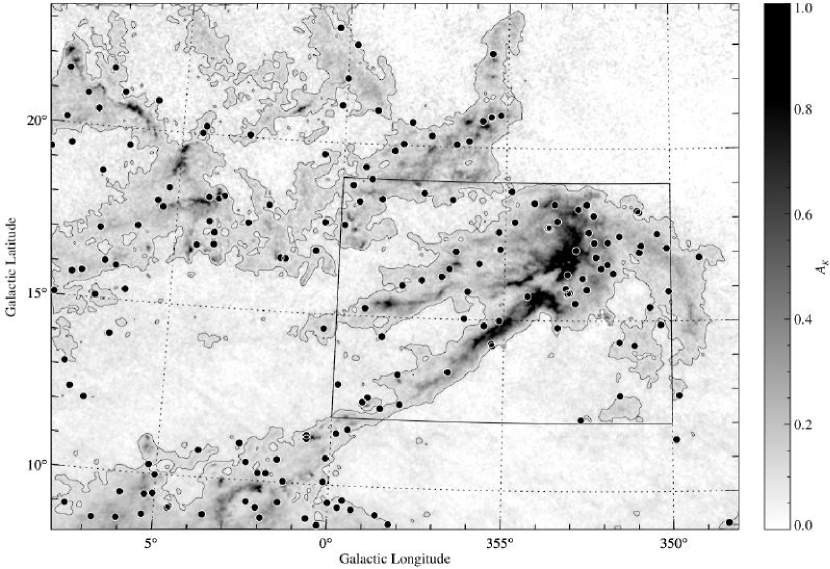
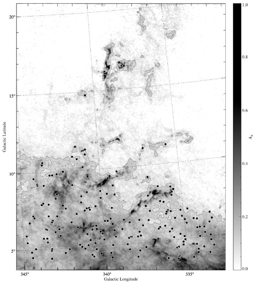
Our technique is based on a simple fact: stars observed through high column-densities must exhibit a significant reddening, while foreground stars will show no reddening even when observed in projection toward dense regions of the cloud. The first step was thus to make reliable extinction maps of the $\rho$-Ophiuchi and Lupus clouds in order to delineate the cloud boundaries and regions to be considered for the distance analysis. For the purpose, we used approximately $42$ million stars from the Two Micron All Sky Survey (2MASS) point source catalog to construct a $1\,672$ square degrees Nicer (Lombardi & Alves, 2001) extinction map of the Ophiuchus and Lupus dark nebulæ. The map, described elsewhere (Lombardi et al., 2008), a has a resolution of $3\mbox{ arcmin}$ and a $3\sigma$ detection level of $0.5$ visual magnitudes. We considered the two regions shown in Figs. 1 and 2, approximately corresponding to the galactic coordinates

$$-12^{\circ}<l {}<2^{\circ} 9^{\circ}<b {}<24^{\circ}$$ (1)

for Ophiuchus, and

$$353^{\circ}<l {}<345^{\circ} 4^{\circ}<b {}<19^{\circ}$$ (2)

for Lupus, and selected there all Hipparcos and Tycho (Perryman et al., 1997) parallax measurements of stars in regions characterized by a relatively high column densities (more precisely, in regions with $A_{K}>0.1\mbox{ mag}$ in our 2MASS extinction map). Finally, in order to estimate the intrinsic colors of the Hipparcos stars, we obtained their spectral types. For the purpose, we used the All-Sky Compiled Catalogue (ASCC-2.5; Kharchenko, 2001), which lists $2\,501\,304$ stars taken from several sources (mainly the Hipparcos-Tycho family, the ground-based Position and Proper Motion family, and the Carlsberg Meridian Catalogs), and the “Tycho-2 Spectra Type Catalog” (Tycho-2spec, III/231; Wright et al., 2003), which cross-references $351\,863$ Tycho stars with spectral catalogues (mainly the Michigan catalogs). In summary, our joined catalog contains for each star observed in projection with relatively large extinction regions the parallax and its related error, the spectral type, and a set of visual magnitudes with errors.

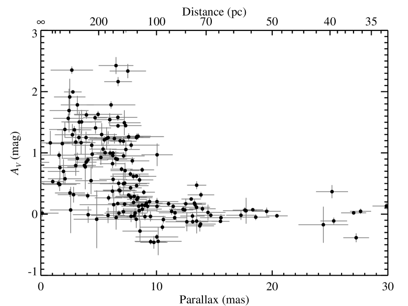
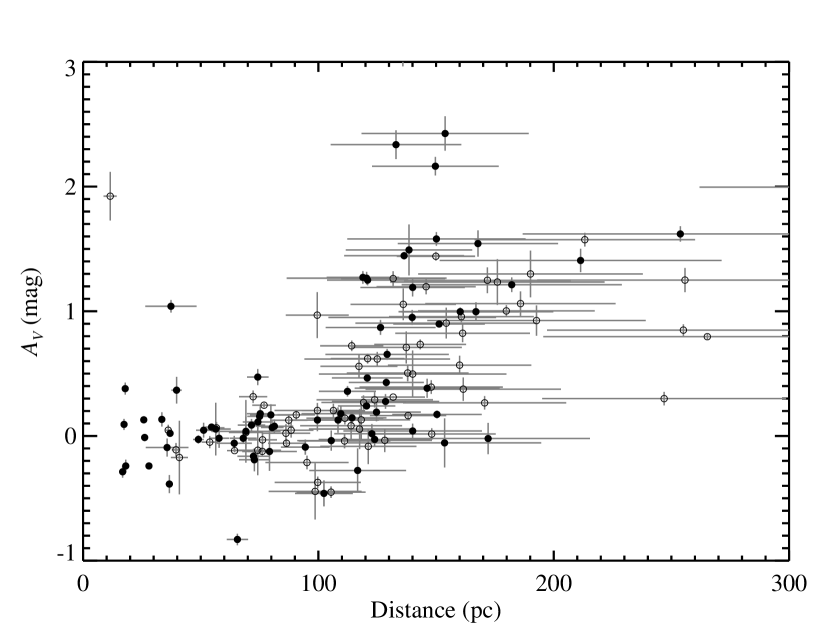
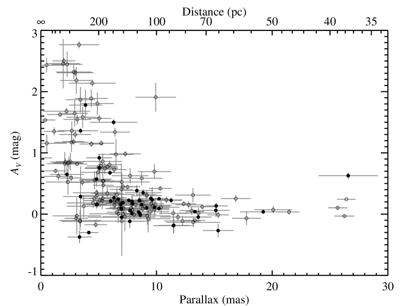
We then considered all Hipparcos stars with well determined parallaxes (we required the parallax error to be smaller than $3\mbox{ mas}$) in the region considered, and estimated the intrinsic $B-V$ of each star from its spectral type (for this purpose, we used the color tables in Landolt-Börnstein, 1982, p. 15, and the normal reddening law of Rieke & Lebofsky, 1985). Finally, we evaluated the extinction of each star by comparing its observed $B-V$ color with its estimated intrinsic color. As final selection, we required stars to have a $V$-band extinction error smaller than $1\mbox{ mag}$, which left 180 objects in the Ophiuchus region, and 186 objects in the Lupus region. A plot of the star column density versus the Hipparcos parallax for both cloud complexes is shown in Figs. 3 and 5; a distance-reddening zoom plot for Ophiuchus is presented in Fig. 4.

Figure 3 proves the effectiveness of the parallax method: from the right to the left, stars are initially found close to the $A_{V}=0\mbox{ mag}$ line, with a relatively low dispersion; then, as we go to smaller parallaxes, an impressive “wall” of stars with significant reddening is observed (approximately at $\pi=8\mbox{ mas}$). Since for Fig. 3 we only selected stars observed against high-column density regions in Ophiuchus, and we further excluded stars with suboptimal measurement errors, the parallax-reddening plot appears extremely clear and gives alone an accurate measurements of the distance of the cloud, that we estimate to be approximately $120\mbox{ pc}$.

The same plot for the Lupus region, shown in Fig. 5, appears to be slightly less clear, for several reasons. First, Lupus has a complex structure and is composed of several subclouds spanning several degrees (see Fig. 2); hence, it is not unlikely that different clouds are located at different distances (see discussion below). In addition, the Lupus cloud complex seems to be at a larger distance than Ophiuchus, at the limit of the Hipparcos sensitivity, and hence the plot of Fig. 5 is perhaps not as crystal clear as the one of Fig. 3. Still, a preliminary qualitative analysis indicates a cloud distance close to $150\mbox{ pc}$ for Lupus.

An intrinsic problem of this technique is that, in this basic formulation, it does not allow a simple, robust estimate of the error associated with the distance measurement. In addition, the value provided must be regarded as an upper limit, since the distance is typically estimated from the first star that shows a significant reddening.

3 Likelihood analysis

Figure 6: The likelihood function of Eq. (6) for Lupus (left black histogram) and Ophiuchus (right black histogram) as a function of the cloud parallax $\pi_{\mathrm{cloud}}$ marginalized over all the other parameters. Both histograms shows marked peaks at $\pi_{\mathrm{Lup}}\simeq 7\mbox{ mas}$ and $\pi_{\mathrm{Oph}}\simeq 9\mbox{ mas}$, corresponding to distances of approximately $119\mbox{ pc}$ and $155\mbox{ pc}$, respectively. The grey histogram refers to the likelihood function for the central region of Ophiuchus (marked window in Fig. 1).

A less qualitative estimate can be obtained by using a statistical model for the parallax-reddening relation. Following Lombardi et al. (2006), we assumed that the $A_{V}$ measurement for foreground stars is small, while a fraction $f$ of the background stars is distributed as a normal variable with relative large mean and variance. Mathematically, we considered the two distributions

$$p^{\mathrm{fg}}(A_{V})={} \mathrm{Gau}(A_{V}|A_{V}^{\mathrm{fg}},\sigma_{A_{V}}^{\mathrm{fg}2}+\sigma_{A_{V}}^{2})\;,$$ (3)

$$p^{\mathrm{bg}}(A_{V})={} \mathrm{Gau}(A_{V}|A_{V}^{\mathrm{bg}},\sigma_{A_{V}}^{\mathrm{bg}2}+\sigma_{A_{V}}^{2})\;,$$ (4)

where we denoted with $\mathrm{Gau}(x|\bar{x},\sigma_{x}^{2})$ the value at $x$ of a normal probability density with mean $\bar{x}$ and variance $\sigma^{2}_{x}$. The two distributions $p^{\mathrm{fg}}$ and $p^{\mathrm{bg}}$ refers to foreground (i.e., almost unextincted) and background (heavily extincted) stars. These are taken to be normal distributions with variances given by the sum of the intrinsic scatter of column densities ($\sigma_{A_{V}}^{\mathrm{fg}2}$ and $\sigma_{A_{V}}^{\mathrm{bg}2}$) and of the measurement error for the star considered ($\sigma_{A_{V}}^{2}$). Note, in particular, that $\sigma_{A_{V}}^{\mathrm{bg}}$ accounts for the local changes in the cloud column density with respect to the average value $A_{V}^{\mathrm{bg}}$, while $\sigma_{A_{V}}^{\mathrm{fg}}$ is introduced to allow for underestimates of the photometric errors on the star magnitudes or for foreground, thin nearby clouds. Finally, the probability distribution $p(A_{V}|\pi)$ for the $A_{V}$ measurement for a star at parallax $\pi$ was taken to be

$$p(A_{V}|\pi)=\begin{cases}p^{\mathrm{fg}}(A_{V})&\text{if $\pi>\pi_{\mathrm{cloud}}\;,$}\\[5.0pt] (1-f)p^{\mathrm{fg}}(A_{V})+fp^{\mathrm{bg}}(A_{V})&\text{if $\pi\leq\pi_{\mathrm{cloud}}\;.$}\end{cases}$$ (5)

Note that the parameter $f\in[0,1]$ denotes the “filling factor,” i.e. the probability that a background star is extincted by the cloud.

We considered this simple model leaving all parameters $\bigl{\{}\pi_{\mathrm{cloud}},f,A_{V}^{\mathrm{fg}},\sigma_{A_{V}}^{\mathrm{fg}},A_{V}^{\mathrm{bg}},\sigma_{A_{V}}^{\mathrm{bg}}\bigr{\}}$ free. In order to assess the goodness of a model, we computed the likelihood function, defined as

$$\mathcal{L}(\pi_{\mathrm{cloud}},f,A_{V}^{\mathrm{fg}},\sigma_{A_{V}}^{\mathrm{fg}},A_{V}^{\mathrm{bg}},\sigma_{A_{V}}^{\mathrm{bg}})={}\\ \prod_{n=1}^{N}\int_{0}^{\infty}p\bigl{(}A_{V}^{(n)}\bigm{|}\pi^{(n)}\bigr{)}p\bigl{(}\pi^{(n)}\bigm{|}\hat{\pi}^{(n)}\bigr{)}\,\mathrm{d}\pi\;,$$ (6)

where the product is carried over all $N$ stars of Figs. 3 and 5, and where $p\bigl{(}\pi^{(n)}\bigm{|}\hat{\pi}^{(n)}\bigr{)}$ is the probability distribution that the $n$-th star with measured parallax $\hat{\pi}^{(n)}$ has a true parallax $\pi^{(n)}$. Note that the integral appearing in Eq. (6) properly takes into account the possibility that a star with a measured parallax $\hat{\pi}^{(n)}<\pi_{\mathrm{cloud}}$ (or $\hat{\pi}^{(n)}>\pi_{\mathrm{cloud}}$) is incorrectly taken as background (respectively, foreground). For this probability we used a normal distribution:

$$p\bigl{(}\hat{\pi}^{(n)}\bigm{|}\pi^{(n)}\bigr{)}=\mathrm{Gau}\bigl{(}\hat{\pi}^{(n)}\bigm{|}\pi^{(n)},\hat{\sigma}_{\pi}^{(n)2}\bigr{)}\;,$$ (7)

where $\hat{\sigma}_{\pi}^{(n)}$ is the estimated error on the parallax. Note that the use of normal distributions in Eqs. (3), (4), and (7) makes it possible to perform the integral (6) analytically in terms of the error function erf.

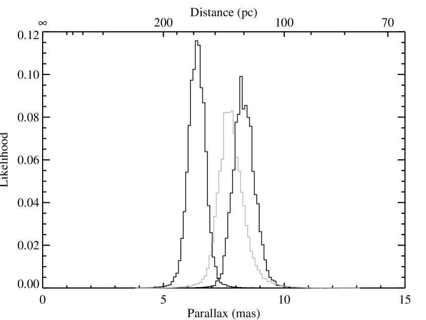
The likelihood function (6) was analysed using Monte Carlo Markov Chains (MCMC; see, e.g. Tanner, 1991). Figure 6 shows the likelihood as a function of the cloud distance, marginalized with respect to all other parameters. From this figure we can trivially evaluate the confidence regions for the estimated distances; in particular, we obtain $d_{\mathrm{Oph}}=(119\pm 6)\mbox{ pc}$, and $d_{\mathrm{Lup}}=(155\pm 8)\mbox{ pc}$, both at the $68\%$ confidence level (since the likelihood function is well approximated by a Gaussian, other confidence bounds can easily derived from the errors quoted here). We stress that the errors quoted here include only statistical errors, as deduced from the parallaxes and reddening uncertainties; other effects, such as the thickness of the cloud or its orientation in the sky are not taken into account and are discussed below in Sect. 4. We stress also that the Lupus distance estimate approximately refers to the average location of background stars in the field (i.e., to $l=339^{\circ}$ and $b=7^{\circ}$), approximately $5.5$ degrees south than the center of the field considered, and that only a few stars are observed through Lupus 1. This difference can play a significant role in case of noticeable tilts in the cloud orientation or in case of multiple components at different distances (see below).

Note that the reliability of the maximum-likelihood technique presented here was also checked with numerical simulations. It is well known that the maximum-likelihood method is, under certain circumstances (verified in our case), asymptotically unbiased; however, we decided to test its behaviour in our specific case, with a limited (although large) number of data. For the purpose, we simulated a “thin” cloud together with observation of a population of stars. We included reasonable errors on both the star parallaxes and column densities, and recovered the distance of the cloud using the same method described here. These simulations confirmed that our estimate is essentially unbiased (i.e., that on average it returns the true distance of the cloud), and that the error provided is reliable.

We also considered a two-screen configuration, with two partially overlapping clouds at different distances, and checked the distance provided by the method. Interestingly, the simulation showed that in this case the method tends to return a “weighted” distance, i.e. a weighted mean of distance of the two screens (where the weights are essentially proportional to the number of stars intercepted by the two screens and by the column densities associated with the two clouds). This result is very encouraging, since it guarantees that, at least in the relatively simple cases considered, the maximum likelihood provide a sensible and unbiased estimate of the cloud distance. Note, however, that the last result also shows that in case of composite clouds with significantly different densities of background stars (e.g., because of their different galactic latitude), the maximum-likelihood technique will be biased toward the distance of the cloud with the highest density of stars. This point is particularly relevant for Lupus, a cloud complex that spans several degrees in galactic latitude, and for which there are indications of possible different distances among the various subclouds (see below Sect. 4.2; cf. also Alves & Franco, 2006).

4 Second order geometrical effects

Given the angular size of the regions considered, it is not unlikely that the cloud complexes have a thickness of $15\mbox{ pc}$ or more. Similarly, even for “thin” clouds, we can easily imagine that they are not perfectly perpendicular to the line of sight and that different regions of them are at different distances. All these geometrical effects can be introduced in the maximum-likelihood analysis discussed above.

4.1 Cloud thickness

The thickness of a molecular cloud can be investigated by modifying the probability distribution of Eq. (5). This can be done in several ways, which corresponds to different “definitions” of the thickness of a cloud. We chose to parametrize the thickness as a continuous, linear transition in the filling factor $f$, which effectively becomes a function of the parallax. Hence, we wrote

$$p(A_{V}|\pi)=f(\pi)p^{\mathrm{bg}}(A_{V})+\bigl{[}1-f(\pi)\bigr{]}p^{\mathrm{fg}}(A_{V})\;,$$ (8)

where

$$f(\pi)=\begin{cases}0&\text{if $\pi>\pi_{1}\;,$}\\[5.0pt] f_{\mathrm{max}}(\pi-\pi_{1})/(\pi_{2}-\pi_{1})&\text{if $\pi_{2}<\pi<\pi_{1}\;.$}\\[5.0pt] f_{\mathrm{max}}&\text{if $\pi<\pi_{2}\;.$}\end{cases}$$ (9)

In other words, stars up to the lower distance of the cloud ($\pi>\pi_{1}$) show no extinction, and thus their column density is distributed according to $p^{\mathrm{fg}}(A_{V})$; similarly, stars background to the cloud ($\pi<\pi_{2}$) follow, with probability $f_{\mathrm{max}}$ (the usual filling factor), a distribution $p^{\mathrm{bg}}(A_{V})$; finally, stars embedded in the cloud ($\pi_{2}<\pi<\pi_{1}$) present an effective filling factors that raises linearly within the cloud from $0$ to $f_{\mathrm{max}}$. Clearly, both parallaxes $\pi_{1}$ and $\pi_{2}$ were taken as free parameters. Note that, similarly to Eq. (5), the use of a simple linear function for $f(\pi)$ guarantees that we can express analytically the integral of Eq. (6).

Figure 7: A density plot of the likelihood of Eq. (6) with for Ophiuchus with the extinction probability distribution (8), as a function of the cloud distance and thickness (the likelihood has been marginalized with respect to all other parameters). The three curves enclose regions of $68\%$, $95\%$, and $99.7\%$ confidence level, while the line-filled corner in the top-left indicate a region that is physically excluded (observer embedded in the cloud). The two plots at the top and at the right show the distance and thickness marginalized probabilities, together with the median value (solid line) and the usual three confidence regions (dashed and dotted lines).

Figure 8: Same as Fig. 7 for Lupus.

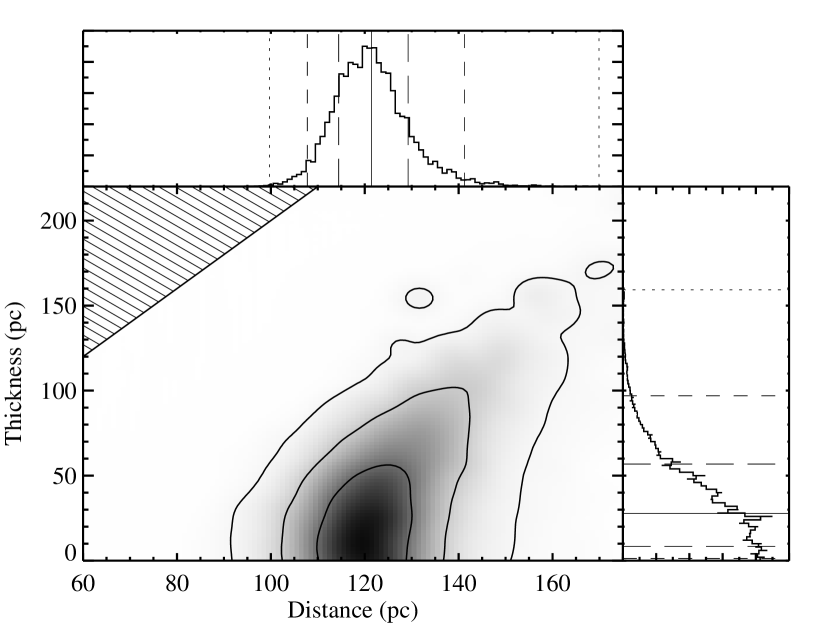
The results of a MCMC analysis of the likelihood function (6) with the distribution of Eq. (8) are shown in Fig. 7 for Ophiuchus and in Fig. 8 for Lupus. The plots in these figures indicate that, unfortunately, the quality and quantity of the available parallaxes is not sufficient to put strong constraints on the thickness of the clouds. In particular, for Ophiuchus we obtained a median thickness of $28^{+29}_{-19}\mbox{ pc}$, but the errors are clearly very large; the situation is even more extreme for Lupus, with a thickness estimate of $51^{+61}_{-35}\mbox{ pc}$. Still, this analysis is important because it can in principle provide different distributions for the distances of the two clouds (see top plots in Figs. 7 and 8) with respect to the ones obtained from the simpler analysis of Sect. 3 (Fig. 6). In this respect, the fact that the two results obtained are almost identical confirms the robustness of our distance estimates. In addition, the much larger thickness estimate for Lupus and the flat plateau evident in the right plot of Fig. 8 suggest that the apparent thickness of Lupus might be the result of different Lupus subclouds being at different distances (see below Sect. 4.2). Finally, we note that the method proposed here to study the cloud thickness will certainly provide much more interesting results when a large statistics of high-quality parallaxes will become available.

4.2 Cloud orientation (tilt)

In order to investigate the presence of possible tilts in the orientation of molecular clouds, we considered a simple model of a thin cloud located at a distance that is a linear function of the sky coordinates:

$$d(x,y)=d_{0}+d_{x}x+d_{y}y\;.$$ (10)

In this equation, $d_{0}$ is the distance of the cloud at a reference point (typically, the center of the region considered), and the sky coordinates $(x,y)$ are taken to be measured in pc and oriented along the horizontal and vertical axes of Figs. 1 and 2 (so that $d_{x}$ and $d_{y}$ are pure numbers). This simple prescription can be directly introduced in Eq. (5) without any further significant modification of the model.

Figure 9: A density plot of the derived probability distribution for the tilt parameters $d_{x}$ and $d_{y}$ of Eq. (10) in Ophiuchus. Similarly to Fig. 7, the three curves enclose regions of $68\%$, $95\%$, and $99.7\%$ confidence level and the two plots at the top and at the right show the X tilt and Y tilt marginalized probabilities.

Figure 10: Same as Fig. 9 for Lupus.

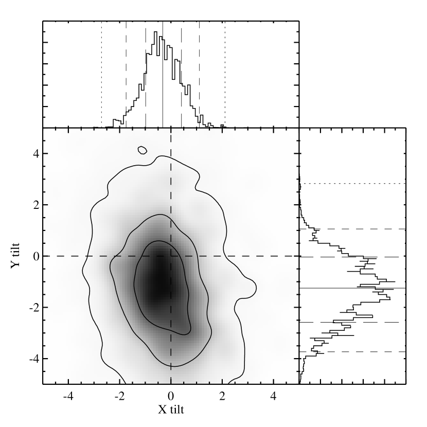
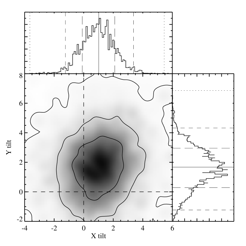
We studied again this model with MCMC and obtained the probability distribution for $(d_{x},d_{y})$ shown in Figs. 9 and 10. In summary, for Ophiuchus we marginally detected a small tilt oriented such that the Ophiuchus streamers would be closer to us than the $\rho$ Ophiuchi core. Indeed, if we repeat the simple analysis of Sect. 3 to the window marked with a solid line in Fig. 1, the denser central regions of Ophiuchus that include the well known $\rho$ Oph core, the distance estimate increases to $(128\pm 8)\mbox{ pc}$. In contrast, for Lupus we detect a vertical gradient in the distance, with the high-galactic latitude regions at larger distances than the low-galactic latitude ones (note that, according to the right plot of Fig. 10, the gradient in galactic latitude is detected at a $3\sigma$ level). Hence, this result together with the large extent of Lupus on the sky seems to indicate that this complex might not be composed of physically related clouds, as also proposed by Bertout et al. (1999) and Knude & Nielsen (2001). Unfortunately, in the current form the method presented here cannot automatically distinguish multiple components of a cloud complex located at different distances. Of course, it is always possible to repeat the analysis in different subclouds, but this requires an a priori assumption on the subcloud division. For Lupus subclouds at high galactic latitudes, in particular, this is manifestly not viable given the relatively small number of stars present there. As described above, we applied this technique to the central region of the Ophiuchus complex, obtaining a somewhat higher distance for it. We also considered subregions of Ophiuchus occupying different sectors of Fig. 1 (defined by the two diagonals, the central vertical line, and the central horizontal line). However, within the relatively large errors of these analyses, we could not identify any significant difference in the distance. Note that this result is consistent with large errors shown by the plot of Fig. 9, which shows that a “flat” screen molecular cloud is still consistent with our data.

4.3 Effects of diffuse ISM

So far, in our analysis we have implicitly assumed that the only significant extinction is associated with the molecular cloud. In reality, the dust present in the interstellar medium (ISM) is known to produce an average $V$-band extinction of approximately $1\mbox{ mag kpc}^{-1}$ along the galactic plane. In principle, it is not difficult to take into account this effect by replacing Eqs. (3) and (4) with

$$p^{\mathrm{fg}}(A_{V}|\pi)={} \mathrm{Gau}(A_{V}|A_{V}^{\mathrm{fg}}+\alpha/\pi,\sigma_{A_{V}}^{\mathrm{fg}2}+\sigma_{A_{V}}^{2})\;,$$ (11)

$$p^{\mathrm{bg}}(A_{V})={} \mathrm{Gau}(A_{V}|A_{V}^{\mathrm{bg}}+\alpha/\pi,\sigma_{A_{V}}^{\mathrm{bg}2}+\sigma_{A_{V}}^{2})\;,$$ (12)

where $\alpha\simeq 1\mbox{ mag mas}$. In practice, however, given the relatively large scatter $\sigma_{A_{V}}^{\mathrm{fg}}$ of $A_{V}^{\mathrm{fg}}$ compared to $\alpha/\pi$ for the cloud considered in this paper, the effect of the ISM can be safely neglected for the foreground star probability distribution $p^{\mathrm{fg}}$. In reality, we argue that the same conclusion applies also to the background distribution $p^{\mathrm{bg}}$. First, we note that the large majority of Hipparcos stars have relatively large parallaxes: for example, in the Ophiucus region we found only 10 objects out of 180 with parallaxes larger than $2\mbox{ mas}$. In addition, the combined effect of a large scatter in $\sigma_{A_{V}}^{\mathrm{bg}}$ of $A_{V}^{\mathrm{bg}}$ and of the filling factor $f$ makes the detection of a gradient in $A^{\mathrm{bg}}$ currently unrealistic. A specific maximum-likelihood analysis using Eqs. (11) and (12) has been carried out, and the results show that the arguments just presented hold. In particular, no significant differences in the distance determinations were found using either a fixed $1\mbox{ mag mas}$ or a variable value for $\alpha$.

We stress, however, that with the advent of GAIA, it will be possible to apply the method described in this paper to significantly more distant clouds, for which the cumulative effect of the diffuse ISM can play a relevant role.

5 Discussion

Our analysis indicates that the Ophiuchus cloud is very likely to be closer than the we think: the “standard” distance, $160\mbox{ pc}$, is indeed excluded at $5\sigma$. Not surprisingly, our estimate is in excellent agreement with the one obtained by Knude & Hog (1998) using a similar technique (but note that the two results are based on a different datasets and use different statistical methods).

Recently, Wilson (2002) and Mamajek (2007) reported an Hipparcos estimated distance of Ophiuchus of $d=136^{+8}_{-7}\mbox{ pc}$ and $d=135^{+8}_{-7}\mbox{ pc}$, respectively, results which are marginally in agreement with our distance estimate of the Ophiuchus core. Mamajek mainly focused on the Lynds 168 cloud, and inferred the cloud distance from the parallaxes of seven stars presumably associated with illuminated nebulae. Although his method is plagued by a potential uncertainty, the real association between the Hipparcos stars and the Ophiuchus cloud complex, and suffers from the small number statistics (7 parallaxes), the agreement obtained is reassuring and suggests that we finally have in hand a reliable estimate of the Ophiuchus cloud complex. Wilson (2002), instead, used a more rigorous maximum-likelihood approach, but his analysis is substantially different from ours. In particular, his method is based on a preliminary classification of stars as foreground and background based on their observed reddening; the distance of the cloud is then inferred from the constraints imposed by the parallaxes of the stars considered. In contrast, in our method we do not need to explicitly classify stars, but on the contrary can use directly all data in the likelihood (an advantage of this is that we are able to use in our method also stars that cannot be uniquely classified as foreground or background because, e.g., of their large photometric errors).

Very recently, Loinard et al. (2008) used phase-referenced multi-epoch Very Long Baseline Array (VLBA) observations to measure the trigonometric parallax of the Ophiucus star-forming region. Their method is based on accurate (to better than a tenth of a milli-arcsecond), absolute measurements of the position of individual magnetically active young stars though to be associated with the star-forming region. If multi-epoch data are available, one can infer the parallax of the star, and thus of the star-forming regions, with exquisite accuracy (below $1\mbox{ pc}$ for objects within $\sim 200\mbox{ pc}$). This technique was applied to four stars in the $\rho$-Ophiuchi region, and interestingly it lead to somewhat contradictory results: two objects associated with the sub-condensation Oph A (S1 and DoAr21) have a measured parallax close to $\sim 120\mbox{ pc}$, and thus in excellent agreement with our estimate; two others, associated with the condensation Oph B (VSSG14 and VL5), have a much higher distance of $\sim 165\mbox{ pc}$. A possible explanation of this is provided by a closer examination of the two sources in the Oph B condensation. From their spectral energy distributions (SEDs), they appear to be Class III A-type stars, with little or no circumstellar emitting dust, and an extinction as large as $50\mbox{ mag}$ in the $V$ band (see Wilking et al., 1989, and especially Greene et al., 1994 for a discussion on the individual SEDs of VSSG14 and VL5). These results indicate that VSSG14 and VL5 are probably background stars, not directly associated with the Ophiucus complex, and likely to be part of a smaller OB association at $\sim 165\mbox{ pc}$.

The distance of the Lupus complex is substantially in agreement with the ones reported in the literature, but both the thickness analysis and the orientation analysis suggest noticeable differences in the various Lupus subclouds.