WIS/02/08-JAN-DPP

On the Conformal Field Theory Duals of type IIA
$AdS_{4}$ Flux Compactifications

Ofer Aharony, Yaron E. Antebi, Micha Berkooz

Department of Particle Physics,
Weizmann Institute of Science, Rehovot 76100, Israel

E-mails : Ofer.Aharony@weizmann.ac.il, ayaron@weizmann.ac.il, Micha.Berkooz@weizmann.ac.il

We study the conformal field theory dual of the type IIA flux compactification model of DeWolfe, Giryavets, Kachru and Taylor, with all moduli stabilized. We find its central charge and properties of its operator spectrum. We concentrate on the moduli space of the conformal field theory, which we investigate through domain walls in the type IIA string theory. The moduli space turns out to consist of many different branches. We use Bezout’s theorem and Bernstein’s theorem to enumerate the different branches of the moduli space and estimate their dimension.

1 Introduction and Summary of Results

Flux compactifications of string theory (for reviews see [1, 2, 3, 4, 5, 6]) populate large parts of the string landscape, and may describe our universe. However, the theoretical basis for the construction of these compactifications is still far from rigorous (see [7] for criticism), and is based on using low-energy supergravity actions in a regime which is different from the flat-space regime where they are usually derived from string theory. It would be very interesting if a non-perturbative construction of some flux compactifications could be found, providing further support for their consistency, and perhaps leading to new methods for their analysis. A promising arena for such a construction is in flux compactifications involving four dimensional anti-de Sitter (AdS) space. Such compactifications are dual, by the AdS/CFT correspondence [8, 9, 10], to three dimensional conformal field theories. Thus, understanding the three dimensional conformal field theory dual to some $AdS_{4}$ flux compactification would give a non-perturbative definition for that background. Eventually we would like to study the statistics of conformal field theories that are dual to $AdS_{4}$ backgrounds, in order to learn about statistics of flux compactifications, and to try to understand how to describe also backgrounds with a positive cosmological constant.

For general flux compactifications, it seems that understanding the dual conformal field theory must be very complicated (see [11, 12] for attempts in this direction). This is because the cosmological constant of the resulting background, which is related to the central charge of the dual conformal field theory, depends in a very complicated way on the fluxes, and it seems that extremely complicated dynamics is needed to reproduce this on the field theory side. The situation seems to be much simpler in the type IIA flux compactifications constructed in [13] (these solutions were further analyzed from the ten dimensional point of view in [14, 15]). These backgrounds have a “large-flux limit” in which some of the fluxes (the three four-form fluxes $f_{4}^{1}$, $f_{4}^{2}$ and $f_{4}^{3}$) are taken to be large, such that in that limit the cosmological constant becomes small, the string coupling becomes weak, and the compact space becomes large. This means that these backgrounds can reliably be studied in the supergravity approximation (except perhaps near the orientifold where the string coupling may be large), and that in the “large-flux limit” the properties of the dual conformal field theories depend in a simple way on the fluxes. One can then hope to reproduce this simple dependence in some field theoretic model. A first attempt at such an analysis, in a different “large-flux limit” which does not lead to a weakly coupled string theory (not all four-form fluxes are taken to be large) appeared in [16]; we will attempt here to describe the field theories appearing in the generic “large-flux limit”, which is described by a weakly coupled string theory.

The naive way to construct a field theory dual for flux backgrounds is to imagine constructing the flux gradually from branes carrying that flux, in a manner similar to that in which the $AdS_{5}\times S^{5}$ background of string theory is constructed from D3-branes in flat space. In particular, the 4-form fluxes $f_{4}^{i}$ in our background are carried by D4-branes wrapped on 2-cycles in the compact space, and it is natural to imagine building the background from such D4-branes [11, 12, 17]. It is certainly possible to go from a background with a large flux (which is already a weakly coupled weakly curved background) to a background with an even larger flux by adding such branes, and we will use this in our discussion of the moduli space of the conformal field theory. However, it is not clear if one can construct the full theory from such branes, since in the limit of a small flux the background becomes not only strongly curved (this happens also for D3-branes) but also strongly coupled. Nevertheless, it is still natural to guess that the dual conformal field theory arises from some decoupled low-energy theory living on three sets of D4-branes. However, we will find that assuming that the degrees of freedom in this theory are weakly coupled open strings (in adjoint and bi-fundamental representations of the resulting $U(f_{4}^{1})\times U(f_{4}^{2})\times U(f_{4}^{3})$ gauge theory) leads to a contradiction, since the central charge of the dual conformal field theory (which scales as $(f_{4}^{1}f_{4}^{2}f_{3}^{3})^{3/2}$, as we will compute in section 3) grows faster than the number of such degrees of freedom. Thus, the field theory must be more complicated than the naive theory of open strings, perhaps involving a larger gauge group, or [12] fields in multi-fundamental or other higher representations, or perhaps not coming from any gauge theory at all.

In order to find clues about this mysterious field theory we investigate in some detail its moduli space, which can be described using configurations of domain walls in $AdS_{4}$. Of course, generic flux backgrounds preserve no supersymmetry so they would not be expected to have a moduli space. The flux backgrounds of [13] preserve a four dimensional ${\cal N}=1$ supersymmetry, so they are dual to three dimensional ${\cal N}=1$ superconformal field theories. This amount of supersymmetry is not enough to protect the moduli space from quantum corrections, since generic scalar potentials are consistent with three dimensional ${\cal N}=1$ supersymmetry. Nevertheless, in our study (performed in the weak coupling weak curvature limit) we will find a large moduli space in these backgrounds. We expect this moduli space to be lifted by quantum corrections (perhaps non-perturbative), but these quantum corrections are small in the “large flux limit”, and we expect the existence of a moduli space in this limit to be a useful clue for the construction of the dual field theory. The moduli space turns out to be very complicated, with many different branches that may be interconnected. For each such branch we employ some mathematical theorems that count the number of solutions of polynomial equations, in order to compute its dimension. We will show that for large values of the fluxes, the dimension of the moduli space scales as $\sum_{i<j}f_{4}^{i}f_{4}^{j}$.

The effective field theory at generic points on the moduli space includes $U(1)$ gauge fields, scalars and fermions; however, in $2+1$ dimensions a $U(1)$ gauge field is equivalent to a compact scalar, so the presence of these gauge fields does not necessarily imply that the full theory is related to a $U(f_{4}^{1})\times U(f_{4}^{2})\times U(f_{4}^{3})$ gauge theory. However, there are special submanifolds of the moduli space in which we can see gauge groups corresponding to all subgroups of $U(f_{4}^{1})\times U(f_{4}^{2})\times U(f_{4}^{3})$, suggesting that the conformal field theory may be described as the low-energy limit of some gauge theory which includes this gauge group. This is further supported by the scaling of the dimension of the moduli space, that is reminiscent of strings in the bi-fundamental representation of each pair of gauge groups (and such bi-fundamental fields indeed appear on the special submanifolds mentioned above).

So far we have not been able to find a simple field theory model that would reproduce all the properties that we find; in particular it seems hard to explain the large number of degrees of freedom, and the complicated form of the moduli space. We hope that these properties will provide useful clues for the construction of such a field theory in the future.

We begin in section 2 with a review of the type IIA backgrounds of [13] that we will be studying and of their supersymmetry equations. In section 3 we compute various basic properties of the dual field theory, like its central charges and the generic features of its operator spectrum. In section 4 we consider branes spanning domain walls in the $AdS_{4}$ space, and find the condition that they preserve supersymmetry. We then go on in section 5 to study the structure of their moduli space. We compute the moduli space explicitly for a simple example and find some properties, such as the dimension, for the generic case. In the appendices we include some additional calculations, including an explicit calculation of the supersymmetry in the bulk in appendix A. In appendix B we show that the domain walls found in section 4 obey the BPS condition, and in appendix C we consider the possibility of additional domain wall brane configurations.

2 The Model

In this section we review the low-energy limit of the background of massive type IIA string theory described by an orientifold of type IIA string theory on $T^{6}/\mathbb{Z}_{3}^{2}$. This model was studied extensively in [13], where it was shown that by turning on generic values for the background fluxes it is possible to stabilize all moduli without the use of non-perturbative effects. We will start by reviewing the geometrical properties of the compact manifold, and then discuss the possible moduli and the way in which they can be stabilized. Finally we will show that the background satisfies the supersymmetry equations in the bulk.

2.1 The Geometry

The compact space is an orbifold of $T^{6}$. We parameterize the torus by the three complex coordinates $z_{i}=x_{i}+iy_{i}$, with $i=1,2,3$. We take the complex structure moduli of the tori to be $\tau_{i}=\alpha\equiv e^{2\pi i/6}$, so that the $z_{i}$ coordinates are periodic with the identifications

$$z_{i}\simeq z_{i}+1\simeq z_{i}+\alpha.$$ (2.1)

At this point in the moduli space of the torus, the $T^{6}$ has a $\mathbb{Z}_{3}$ symmetry, under which the coordinates transform as

$$z_{i}\to\alpha^{2}z_{i}.$$ (2.2)

It is then possible to orbifold by this symmetry. This gives rise to a singular space, with 27 singular points corresponding to the fixed points of the $\mathbb{Z}_{3}$ symmetry [18, 19]. After this identification, there is a second $\mathbb{Z}_{3}$ symmetry acting freely on the coordinates as

$$(z_{1},z_{2},z_{3})\to(\alpha^{2}z_{1}+\frac{1+\alpha}{3},\alpha^{4}z_{2}+\frac{1+\alpha}{3},z_{3}+\frac{1+\alpha}{3}).$$ (2.3)

This symmetry identifies triplets of fixed points, thus leading, after a second orbifold by the second $\mathbb{Z}_{3}$ symmetry, to a singular Calabi-Yau manifold with only 9 singular points (that can be locally described as a $C^{3}/\mathbb{Z}_{3}$ singularity). The cohomology of this manifold is given by $h^{2,1}=0$ and $h^{1,1}=12$. There are therefore no complex structure moduli and 12 Kähler moduli. Nine of them are associated to blow-up modes of the singular points, while the other three Kähler moduli describe the volume of the three tori. These volume moduli $\gamma_{i}$ appear in the metric as

$$ds^{2}=\sum_{i=1}^{3}\gamma_{i}dz^{i}d\bar{z}^{i},$$ (2.4)

or in the Kähler form for the manifold as

$$J=ig_{i\bar{j}}\ dz^{i}\wedge d\bar{z}^{j}=\sum_{i=1}^{3}i\frac{\gamma_{i}}{2}dz^{i}\wedge d\bar{z}^{i}.$$ (2.5)

It will be useful to write an explicit basis for the cohomology of the compact space. There are no one-forms, since the two $\mathbb{Z}_{3}$ orbifolds project out all of the one-forms of the torus. There are three two-forms that form the basis of the untwisted part of $H^{2}$. These are the two-forms that remain invariant under the $\mathbb{Z}_{3}^{2}$, and they can be chosen as

$$w_{i}=(\kappa\sqrt{3})^{1/3}idz^{i}\wedge d\bar{z}^{i},$$ (2.6)

in an arbitrary normalization (in which the triple intersection is $\kappa$). Their Poincaré-dual four-forms form the basis for the untwisted part of $H^{4}$,

$$\tilde{w}^{i}=\left(\frac{3}{\kappa}\right)^{1/3}(idz^{j}\wedge d\bar{z}^{j})\wedge(idz^{k}\wedge d\bar{z}^{k}),$$ (2.7)

where $\{i,j,k\}$ are different elements of the set $\{1,2,3\}$. We choose the normalizations such that

$$\int_{T^{6}/\mathbb{Z}_{3}^{2}}w_{1}\wedge w_{2}\wedge w_{3}=\kappa,\qquad\int_{T^{6}/\mathbb{Z}_{3}^{2}}w_{i}\wedge\tilde{w}^{j}=\delta_{i}^{j}.$$ (2.8)

There are also two-forms and four-forms associated with the blow-up modes of the orbifold fixed points, which we will not write down explicitly.

Since $h^{2,1}=0$, the only 3-forms in the compact geometry are the holomorphic 3-form

$$\Omega=\sqrt{\gamma_{1}\gamma_{2}\gamma_{3}}idz_{1}\wedge dz_{2}\wedge dz_{3}$$ (2.9)

and its complex conjugate $\bar{\Omega}$. These are normalized such that

$$\frac{i}{8}\int_{T^{6}/\mathbb{Z}_{3}^{2}}\Omega\wedge\bar{\Omega}=vol(T^{6}/\mathbb{Z}_{3}^{2})=\frac{1}{8\sqrt{3}}\gamma_{1}\gamma_{2}\gamma_{3},$$ (2.10)

and can be verified to obey the standard relations

$$J\wedge\Omega=0,\quad\frac{i}{8}\Omega\wedge\bar{\Omega}=\frac{1}{3!}J^{3}.$$ (2.11)

As a last step in defining the geometry we quotient by an orientifold action. We will use the orientifold of $T^{6}/\mathbb{Z}_{3}^{2}$ presented in [20]. The total orientifold action is given by $\Omega(-1)^{F_{L}}\sigma$, where $\Omega$ is reflection on the worldsheet, $F_{L}$ is the worldsheet left moving fermion number, and $\sigma$ is the spacetime involution

$$z_{i}\to-\bar{z}_{i}.$$ (2.12)

Under this action there is a 3 dimensional space left fixed, given by $\,\mathcal{R}\mathrm{e}\!\left[z_{i}\right]=0$. Thus, the theory contains an $O6$-plane wrapping this 3-cycle and filling the non compact directions.

Under the orientifold action the different forms have non trivial transformation properties. The forms defined above transform as

$$w_{i}\to-w_{i},\qquad\tilde{w}^{i}\to\tilde{w}^{i},\qquad\Omega\to\bar{\Omega}.$$ (2.13)

One can write the three-forms in a diagonal basis with respect to the orientifold by decomposing $\Omega$ to its real and imaginary parts, $\Omega=\frac{\sqrt{\gamma_{1}\gamma_{2}\gamma_{3}}}{3^{1/4}\sqrt{2}}(\alpha_{0}+i\beta_{0})$. These transform as

$$\alpha_{0}\to\alpha_{0},\qquad\beta_{0}\to-\beta_{0}.$$ (2.14)

2.2 Moduli and Their Stabilization

In order to stabilize all the moduli we will need to turn on a 10-form (or 0-form) RR flux, so that in the low-energy limit we obtain Romans’ massive IIA supergravity theory [21] (with a mass parameter proportional to the RR 0-form field strength), compactified to four dimensions on the $T^{6}/\mathbb{Z}_{3}^{2}$ orientifold discussed in the previous subsection. In addition to the background metric and dilaton, the theory includes a NS-NS 2-form $B_{2}$ (whose field strength is $H_{3}$), and a RR 1-form and 3-form, $C_{1}$ and $C_{3}$ (with field strengths $F_{2}$ and $F_{4}$).

Before turning on fluxes, the massless spectrum includes the Kähler parameters from the metric, $\gamma_{i}$, and the dilaton $\phi$. Since $B_{2}$ is odd under $\Omega$, its zero modes are related to the forms $\omega_{i}$ in the $\sigma$-odd cohomology $H^{2}_{-}$, and it can be expanded as

$$B_{2}=\sum b_{i}\omega^{i}.$$ (2.15)

The three zero modes $b_{i}$ combine with $\gamma_{i}$ to form the bosonic part of a chiral multiplet. Similarly we can expand the RR forms. Since $h^{1}=0$, the one-form has no zero modes. The three-form, being even under $\Omega$, has one zero mode, related to the unique even three-form, $\alpha_{0}$. Thus we have

$$C_{3}=\xi\alpha_{0}.$$ (2.16)

The four dimensional axiodilaton superfield contains the combination of this axion $\xi$ with the dilaton $\phi$.

All of these moduli can be stabilized by turning on fluxes along the compact directions. In order to preserve Poincaré invariance, the fluxes can be written as

$$F_{n}=\hat{F}_{n}+vol_{4}\wedge\tilde{F}_{n-4},$$ (2.17)

where all the indices in $\hat{F}$ and $\tilde{F}$ are internal, and they are Poincaré dual using the 6 dimensional metric, $\tilde{F}_{n}=(-1)^{(n-1)(n-2)/2}*_{6}\hat{F}_{6-n}$. The background values for the fluxes can then be written by expanding the fields in the relevant cohomology (having the correct parity under the orientifold) :

$$H_{3}=-p\beta_{0},\quad\hat{F}_{0}=-m_{0},\quad\hat{F}_{2}=-m_{i}w_{i},\quad\hat{F}_{4}=e_{i}\tilde{w}^{i},\quad\hat{F}_{6}=-e_{0}\frac{\alpha_{0}\wedge\beta_{0}}{\rm vol}.\quad$$ (2.18)

They obey the following integrality condition

$$\frac{\sqrt{2}}{(2\pi\sqrt{\alpha^{\prime}})^{p-1}}\int F_{p}=f_{p}\in\mathbb{Z}\ ,\qquad\frac{1}{(2\pi)^{2}\alpha^{\prime}}\int H_{3}=h_{3}\in\mathbb{Z},$$ (2.19)

so that the integer fluxes are related to the ones in (2.18) by

$$f_{0}=-\sqrt{2}2\pi\sqrt{\alpha^{\prime}}m_{0},\qquad f_{2}^{i}=-\frac{\sqrt{2}\kappa^{1/3}}{2\pi\sqrt{\alpha^{\prime}}}m_{i},\qquad f_{4}^{i}=\frac{\sqrt{2}}{\kappa^{1/3}(2\pi\sqrt{\alpha^{\prime}})^{3}}e_{i},$$ (2.20)

$$\hskip 70.0ptf_{6}=-\frac{\sqrt{2}}{(2\pi\sqrt{\alpha^{\prime}})^{5}}e_{0},\qquad h_{3}=\frac{1}{(2\pi\sqrt{\alpha^{\prime}})^{2}}p.$$ (2.21)

We will split the field strengths into the background part and an excitations part. They can then be written as

$$H_{3} = H_{3}^{bg}+dB_{2},$$ (2.22)

$$F_{2} = F_{2}^{bg}+dC_{1}+m_{0}B_{2},$$ (2.23)

$$F_{4} = F_{4}^{bg}+dC_{3}-C_{1}\wedge dB_{2}-\frac{m_{0}}{2}B_{2}\wedge B_{2}.$$ (2.24)

The background values of the fluxes are constrained by the tadpoles of the different fields. These were analyzed in [13], where it was found that there is a unique tadpole for $C_{7}$ which requires

$$m_{0}p=-\sqrt{2}\,2\pi\sqrt{\alpha^{\prime}}.$$ (2.25)

In terms of the integer fluxes (2.20) this means $f_{0}h_{3}=2$, so that there are four different possibilities, $(f_{0},h_{3})=(1,2),(2,1),(-1,-2),(-2,-1)$. All other fluxes are not constrained by tadpoles.

The scalar potential was analyzed in detail in [13], and it was found that by turning on such fluxes $(e_{0},e_{i},m_{0},m_{i},p)$ the moduli are stabilized at values given by

$$\gamma_{i} = 2(\kappa\sqrt{3})^{1/3}\frac{1}{|\hat{e}_{i}|}\sqrt{\frac{-5\hat{e}_{1}\hat{e}_{2}\hat{e}_{3}}{3m_{0}\kappa}},$$ (2.26)

$$b_{i} = \frac{m_{i}}{m_{0}},$$ (2.27)

$$e^{-\phi} = \frac{4}{3}\frac{1}{|p|}\left(-\frac{12}{5}\frac{m_{0}\hat{e}_{1}\hat{e}_{2}\hat{e}_{3}}{\kappa}\right)^{1/4},$$ (2.28)

$$\xi = \frac{1}{p}\left(e_{0}+\frac{e_{i}m_{i}}{m_{0}}+\frac{2\kappa m_{1}m_{2}m_{3}}{m_{0}^{2}}\right),$$ (2.29)

with $\hat{e}_{i}\equiv e_{i}+\kappa m_{j}m_{k}/m_{0}$ (where $\{i,j,k\}=\{1,2,3\}$). From the four dimensional point of view, this solution has a negative cosmological constant

$$\Lambda=-\frac{p^{2}}{2}\frac{\sqrt{3}}{\gamma_{1}\gamma_{2}\gamma_{3}},$$ (2.30)

and we will consider the maximally symmetric solution of the resulting four dimensional action, which is given by $AdS_{4}\times T^{6}/\mathbb{Z}_{3}^{2}$.

There are several things to note here regarding this solution. From supersymmetry we get (see the next subsection) a constraint on the signs of the fluxes

$${\rm sign}(m_{0}p)={\rm sign}(m_{0}e_{i})=-,$$ (2.31)

which also guarantees that the $\gamma_{i}$ and $e^{-\phi}$ are real. When we take large values for the quantized fluxes, $f_{4}^{i}\gg 1$ (without making some of them much larger than the others), we get to a regime with large volume and weak coupling where we can trust our computation. Throughout this paper we will work in this regime. We also note that there is a non-singular solution with $e_{0}=m_{i}=0$, which has no 2-form and 6-form background fluxes.

There are additional moduli localized near the $C^{3}/\mathbb{Z}_{3}$ singularities. One can turn on $\hat{F}_{2}$ and $\hat{F}_{4}$ fluxes on the corresponding localized cycles, which we denote, respectively, by $n_{A}$ and $f_{A}$ ($A=1,\cdots,9$ goes over the different singular points). The blow up Kähler modes ${t_{B}}_{A}$ are then stabilized at

$${t_{B}}_{A}=\frac{n_{A}}{m_{0}}-i\sqrt{-\frac{10\hat{f}_{A}}{3\beta m_{0}}},$$ (2.32)

where we defined $\hat{f}_{A}\equiv f_{A}+\beta n_{A}^{2}/2m_{0}$, and the integer $\beta$ is the non-trivial triple intersection of the twisted cycles. The values for $e^{\phi}$ and $\xi$ are modified by these additional fluxes (the dilaton by a small amount when $f_{4}^{i}\gg 1$):

$$e^{-\phi} = \frac{4}{3}\frac{1}{|p|}\left[\sqrt{-\frac{12}{5}\frac{m_{0}\hat{e}_{1}\hat{e}_{2}\hat{e}_{3}}{\kappa}}+\frac{3}{25}m_{0}^{2}\beta\sum_{A}\left(-\frac{10f_{A}}{3\beta m_{0}}\right)^{3/2}\right]^{1/2}$$ (2.33)

$$\xi = \frac{1}{p}\left(e_{0}+\frac{e_{i}m_{i}+\sum_{A}f_{A}n_{A}}{m_{0}}+\frac{6\kappa m_{1}m_{2}m_{3}+\beta\sum_{A}n_{A}^{3}}{3m_{0}^{2}}\right).$$ (2.34)

2.3 Supersymmetry

In this subsection we review how the background described above satisfies the supersymmetry equations. We will write the background as a warped product of a four-dimensional Anti de-Sitter space with $T^{6}/\mathbb{Z}_{3}^{2}$, with the metric

$$ds^{2}=e^{2A}h_{MN}dx^{M}dx^{N}+g_{AB}dy^{A}dy^{B},$$ (2.35)

where $A=A(y)$ is the warp factor, $h_{MN}$ is the 4 dimensional AdS metric and $g_{AB}$ is the metric on $T^{6}/\mathbb{Z}_{3}^{2}$. We will use the double spinor convention, which in type IIA amounts to writing the Majorana Killing spinor as two Majorana Weyl spinors with opposite chirality,

$$\epsilon=\epsilon_{+}+\epsilon_{-},\quad\Gamma_{(10)}\epsilon_{\pm}=\pm\epsilon_{\pm}.$$ (2.36)

We can decompose the ten dimensional Clifford algebra into the $4d\otimes 6d$ algebras in the following way,

$$\Gamma_{\underline{\mu}}=\gamma_{\underline{\mu}}\otimes\mathbb{I},\quad\Gamma_{\underline{m}}=\gamma_{(4)}\otimes\hat{\gamma}_{\underline{m}},$$ (2.37)

where the 4d gamma matrices are real and the 6d are purely imaginary and antisymmetric. We denote by underlined indices the tangent space flat indices. The Killing spinors also decompose as

$$\epsilon_{+}(x,y) = a\,\theta_{+}(x)\otimes\eta_{+}(y)+a^{*}\theta_{-}(x)\otimes\eta_{-}(y),$$ (2.38)

$$\epsilon_{-}(x,y) = b^{*}\theta_{+}(x)\otimes\eta_{-}(y)+b\,\theta_{-}(x)\otimes\eta_{+}(y),$$ (2.39)

where $\eta_{+}=\eta_{-}^{*}$ is the unique covariantly constant spinor on the Calabi-Yau, while $\theta_{+}$, $\theta_{-}$ (with $\bar{\theta}_{+}=\theta_{-}^{T}C$) are the Killing spinors on $AdS_{4}$ satisfying

$$D_{\mu}\theta_{+}=\frac{1}{2}\mu^{*}\gamma_{\mu}\theta_{-},\quad D_{\mu}\theta_{-}=\frac{1}{2}\mu\gamma_{\mu}\theta_{+}.$$ (2.40)

The complex number $\mu$ is the value of the superpotential, so that the cosmological constant of the $AdS_{4}$ space is given by $\Lambda=-|\mu|^{2}$.

The spinor $\eta_{+}$ on the Calabi-Yau gives rise to an $SU(3)$ structure. Following [23, 24, 25, 26] we can write the two pure spinors as bispinors of $O(6,6)$ in the following way

$$/\!\!\!\!\Psi^{+}=a\eta_{+}\otimes b^{*}\eta_{+}^{\dagger},\qquad/\!\!\!\!\Psi^{-}=a\eta_{+}\otimes b\eta_{-}^{\dagger}.$$ (2.41)

Using the Clifford map, there is a one-to-one correspondence between such bispinors and p-forms, given by

$$C\equiv\sum\frac{1}{k!}C_{i_{1},\ldots,i_{k}}dx^{i_{1}}\wedge\ldots\wedge dx^{i_{k}}\quad\longleftrightarrow\quad/\!\!\!\!C\equiv\sum\frac{1}{k!}C_{i_{1},\ldots,i_{k}}\gamma_{\alpha\beta}^{i_{1}\ldots i_{k}}.$$ (2.42)

Using this map, the pure spinors can also be represented by the almost complex structure 2-form and the holomorphic 3-form,

$$\Psi^{+}=\frac{a\bar{b}}{8}e^{-iJ},\qquad\Psi^{-}=-\frac{iab}{8}\Omega.$$ (2.43)

Following these notations, the equations for preserved supersymmetry are given by [24, 26]

$$e^{-2A+\phi}(d+H\wedge)(e^{2A-\phi}\Psi_{+}) = 2\mu\,\mathcal{R}\mathrm{e}\!\left[\Psi_{-}\right],$$ (2.44)

$$e^{-2A+\phi}(d+H\wedge)(e^{2A-\phi}\Psi_{-}) = 3i\,\mathcal{I}\mathrm{m}\!\left[\bar{\mu}\Psi_{+}\right]+dA\wedge\bar{\Psi}_{-}$$ (2.46)

$$+\frac{\sqrt{2}}{16}e^{\phi}\left[(|a|^{2}-|b|^{2})\hat{F}+i(|a|^{2}+|b|^{2})\tilde{F}\right],$$

where $F=F_{0}+F_{2}+F_{4}+F_{6}$ are the modified RR fields defined as

$$F=e^{-B}F^{\rm bg}+dC+H\wedge C,$$ (2.48)

so that they obey the non-standard Bianchi identity $dF_{n}=-H\wedge F_{n-2}$.

We solve these equations in Appendix A, finding that for supersymmetry to be preserved the Killing spinors should have $b=-a^{*}$, and the moduli should obtain values as in (2.26).

3 General Properties of the Dual Conformal Field Theory

In the previous section we described a solution of supergravity (and, thus, of string theory) that includes a four dimensional AdS space. According to the AdS/CFT correspondence [8, 9, 10], there is a three dimensional conformal field theory which is the holographic dual of this solution. Many properties of this CFT can be calculated in a simple manner from the supergravity solution. We will discuss these properties in this section, including the central charge, dimensions of operators and the global symmetries of the CFT. We will also discuss D-branes wrapping cycles in the compact space to give particles or strings on $AdS_{4}$. Throughout this paper we will work only in the limit where all 4-form fluxes are large, so that the string coupling is weak and the supergravity approximation is good.

3.1 The Central Charge

We will begin by finding the central charge of the CFT from the curvature of the AdS space. There are various possible definitions of a central charge for three dimensional CFTs, including the coefficient of the two-point function of the stress-energy tensor, and the coefficient multiplying the volume times the temperature squared in the entropy of the theory at finite temperature. In the gravity approximation, all definitions give answers proportional to $R_{AdS}^{2}/G_{4}$, where $G_{4}$ is the four dimensional Newton’s constant, since this is the coefficient (in units of $R_{AdS}$) of the four dimensional action, so that all correlation functions are proportional to this. Using our formulas from the previous section, we have (up to constants)

$$\frac{(R^{AdS}_{4})^{2}}{G_{4}}=\frac{Vol(T^{6}/\mathbb{Z}_{3}^{2})\,e^{-2\phi}\Lambda^{-1}}{\alpha^{\prime 4}}\propto\frac{(f_{4}^{1}f_{4}^{2}f_{4}^{3})^{3/2}}{f_{0}^{5/2}h_{3}^{4}}\simeq(f_{4}^{1}f_{4}^{2}f_{4}^{3})^{3/2},$$ (3.1)

since the 3-form and 0-form fluxes are numbers of order one. In particular, if we take all the fluxes $f_{4}^{i}\sim N$, we find a central charge scaling as $c\propto N^{9/2}$ (this was independently noted in [16]).

Equation (3.1) is reminiscent of the formula for the central charge in the case of ${\cal N}=8$ $SU(N)$ SYM in 2+1 dimensions. In that case the central charge of the theory in the IR (where it is dual to M theory on $AdS_{4}\times S^{7}$) scales like $N^{3/2}$ (which is not understood in terms of any effective field theory degrees of freedom). By analogy, this suggests that in our case there may be some $N_{eff}=f_{4}^{1}f_{4}^{2}f_{4}^{3}$, namely that if there is a UV description of any sort it should include an order of $(f_{4}^{1}f_{4}^{2}f_{4}^{3})^{2}$ degrees of freedom. This is also suggested by the fact that these are the minimal integer powers which are larger than those appearing in the central charge (3.1). This UV description could be for instance an $SU(N_{eff})$ gauge theory, or an $SU(f_{4}^{1})\times SU(f_{4}^{2})\times SU(f_{4}^{3})$ gauge theory with matter in representations whose dimension is of order $N_{eff}^{2}$ (such representations are consistent with asymptotic freedom in $2+1$ dimensions).

The analysis in [16] give some support to this suggestion. It was argued there that after two T-dualities in the directions of the first 2-torus, and in the limit of $f_{4}^{1}\rightarrow\infty,\ f_{4}^{2,3}\ fixed$, the background should be lifted to M theory, and resembles the near-horizon limit of $f_{4}^{1}$ M2-branes (at some singularity). In this case we see that the degrees of freedom are renormalized from $O(1)*(f_{4}^{1})^{2}$ in the theory on some D2-branes (at the same singularity) to $O(1)*(f_{4}^{1})^{3/2}$ in the theory on the M2-branes.

Below we will use another indicator for the number of branes in the problem which will be the structure (and in particular the dimensionality) of different branches of the moduli space. The moduli space will be made out of holomorphic (in an appropriate sense) D4-branes which wrap different 2-cycles of the torus. Our analysis of the moduli space will be performed in the limit where all fluxes are large, but since it preserves some supersymmetry it is natural to expect that the same results for the form and dimension of the moduli space will hold also in other limits (though we have not verified this directly). Assuming this, we find (using our results derived below) that for the scaling of [16] the dimension of the largest branch of the moduli space will scale like $f_{4}^{1}$. Indeed, this branch is described by the motion of D4-branes wrapping the first $T^{2}$, which become M2-branes (or D2-branes) after 2 T-dualities.

Our more general analysis below will show that the dimension of the maximal branch of the moduli space scales like $\max(f_{4}^{i}f_{4}^{j}),\ i\not=j$. The previous case is a special case of this. Note that this might suggest that in a scaling limit in which two of the fluxes (say, $f_{4}^{1}$ and $f_{4}^{2}$) become large while the third remains finite, the theory resembles that of $N_{eff}\simeq f_{4}^{1}f_{4}^{2}$ M2-branes. While the dimension of the moduli space and the number of degrees of freedom are consistent with this suggestion, the precise form of the moduli space is very different from what one would obtain from any theory of $N_{eff}$ M2-branes.

3.2 Global Symmetries

As described above, the supergravity solution preserves a four dimensional ${\cal N}=1$ supersymmetry. By the AdS/CFT correspondence this maps to a three dimensional ${\cal N}=1$ superconformal symmetry, with two supersymmetry charges and two superconformal charges.

In the AdS/CFT correspondence, the global symmetries of the CFT are related to gauge symmetries of the gravitational theory. Such symmetries arise from reductions of the supergravity fields on the compact space (or from space-filling D-branes). The simplest gauge fields are related to the ten dimensional metric, and are related to the isometry group of the compactification manifold. In our case the compact space is a Calabi-Yau manifold and thus has no isometry group. So, we do not get any gauge fields from the metric. In addition to the metric, the RR 1-form and 3-form can also give rise to gauge symmetries. In our background we have a non-trivial 0-form flux which gives a mass to the 1-form (it is swallowed by the 2-form $B_{2}$ which becomes massive). Thus, there is no gauge symmetry associated with the 1-form. In order to get a 1-form gauge field from the 3-form we need to integrate it over a 2-cycle. As the compactification manifold contains three such untwisted 2-cycles, we obtain three commuting gauge fields. However, since the 2-cycles are odd under the orientifolding, these gauge fields are projected out by the orientifold. The gauge fields arising from the twisted 2-cycles are similarly projected out.

Thus, the conformal field theory that we are looking for does not have any global symmetry (beyond the ${\cal N}=1$ superconformal algebra, which does not include any continuous R-symmetry group).

3.3 Operators and Scalings

Another basic property of a conformal field theory is the spectrum of operators in the theory. The simplest operators are related to the supergravity fields, and their dimensions are related to the masses so we can easily find the spectrum. There are two mass scales for fields in the supergravity. The first is the mass of the moduli, which can be computed from their potential. This was written explicitly in [13] for some of the moduli, and it is easy to see that the others have the same scaling. In units of the four dimensional Planck scale $l_{p4}^{2}\simeq G_{4}$ the moduli masses are

$$m^{2}_{moduli}\sim(f_{4}^{1}f_{4}^{2}f_{4}^{3})^{-3/2}l_{p4}^{-2}.$$ (3.2)

The other mass scale in supergravity is the mass of the Kaluza-Klein modes, given by the inverse radii of the compact tori,

$$m^{2}_{KK}\sim\gamma_{i}^{-1}\sim(f_{4}^{1}f_{4}^{2}f_{4}^{3})^{-3/2}f_{4}^{i}l_{p4}^{-2}.$$ (3.3)

The dimensions of the corresponding operators are given using the AdS/CFT correspondence as

$$\Delta_{moduli}\sim m_{moduli}R_{AdS}\sim 1,\qquad\Delta_{KK}\sim m_{KK}R_{AdS}\sim\sqrt{f_{4}^{i}}.$$ (3.4)

Thus, as in all other conformal field theories dual to theories with a four dimensional supergravity approximation (implying a separation of scales between the moduli and the KK modes), there is a small number of operators with dimensions of order one, and all others have large dimensions. The order one operators correspond to the eight moduli fields, $\phi,\xi,b_{i},v_{i}$.

3.4 Wrapped Branes

Another type of operators in the field theory involves D$p$-branes wrapped on $p$-cycles in the compact space, giving particles in the $AdS_{4}$. Since our background involves massive type IIA string theory, we cannot have any D0-branes (which must have $f_{0}$ strings ending on them) or D6-branes (which must have $f_{0}$ NS 5-branes ending on them); this is related to the fact that the RR 1-form is swallowed by the NS-NS 2-form. Naively we can have wrapped D2-branes or D4-branes on our 2-cycles or 4-cycles, but in fact the orientifold maps these to anti-D-branes, so it is unlikely that any stable configurations of this type would exist.

We can also consider a $p$-brane wrapping a $(p-1)$-cycle, leading to a string in $AdS_{4}$ (mapped to some type of flux tube in the conformal field theory). The only such possible configurations are a D4-brane wrapping a 3-cycle and an NS5-brane wrapped on a 4-cycle. A D4-brane wrapped around the $\alpha_{0}$ cycle is mapped to an anti-brane by the orientifold, while a D4-brane wrapping the $\beta_{0}$ cycle is not a consistent configuration, since there is $H_{3}$-flux on that 3-cycle, implying that such D4-branes must have D2-branes ending on them. The same phenomenon arises for NS5-branes wrapped on the 4-cycles, since these have 4-form flux. Note that the fundamental string is also mapped to a string with opposite orientation by the orientifold. Thus, we do not expect to have any stable extended objects in our theory.

4 Supersymmetric Domain Walls

In the next two sections we wish to study the moduli space of the conformal field theory dual to the background described in section 2. To describe the moduli space we need to find Lorentz-invariant configurations with zero energy which have the same asymptotics as the solution described above, but differ in the interior. Usually in the AdS/CFT correspondence such configurations are described by supersymmetric branes sitting at some value of the radial position, giving domain walls in AdS along which the flux which the brane is charged under jumps. Moving along the moduli space of these configurations is described in the field theory side as giving non-trivial vacuum expectation values to operators. Such domain walls break half of the supersymmetry in the bulk; in the conformal field theory they break the superconformal generators and preserve the standard supersymmetry generators.

We will consider here D-brane domain walls, given by D$p$-branes wrapping $(p-2)$-cycles in the compact space, and sitting at fixed radial position in $AdS_{4}$. For the configuration to be supersymmetric (which is the same as having zero energy in the field theory) these must obey some calibration condition [27]. We will find the supersymmetric cycles over which D-branes can be wrapped by considering the $\kappa$-symmetry equation. In Appendix B we will also verify directly that these configurations are BPS states by considering the DBI+CS action for the D-branes and checking that there is no force acting on them. All of these equations are valid in the probe approximation, in which the back-reaction of the D-brane on the background is small. This approximation will be good in the limit of large four-form fluxes that we are working in. Since in three dimensional ${\cal N}=1$ theories the moduli space is generally not protected, we expect some potential along the moduli space to be generated by corrections to our leading order approximation; however, this potential is very small in the limit we are working in, so that there will still be an approximate moduli space in the conformal field theory.

The general supersymmetry condition for a D$p$-brane filling time plus $q$ dimensions and wrapping a $(p-q)$-cycle in the compact directions is the $\kappa$-symmetry equation [28], which in the double spinor notation can be written as in [25, 26]:

$$\hat{\Gamma}_{Dp}\epsilon_{-}=\epsilon_{+},$$ (4.1)

where

$$\hat{\Gamma}_{Dp}=\gamma_{\underline{0\ldots q}}\gamma_{(4)}^{p-q}\otimes\hat{\gamma}^{\prime}_{(p-q)},$$ (4.2)

$$\hat{\gamma}^{\prime}_{(r)}=\frac{1}{\sqrt{{\rm det}(P[g]+{\cal F})}}\sum_{2l+s=r}\frac{\epsilon^{\alpha_{1}\ldots\alpha_{2l}\beta_{1}\ldots\beta_{s}}}{l!s!2^{l}}{\cal F}_{\alpha_{1}\alpha_{2}}\ldots{\cal F}_{\alpha_{2l-1}\alpha_{2l}}\hat{\gamma}_{\beta_{1}\ldots\beta_{s}}.$$ (4.3)

Here, $P[\cdot]$ indicates the pullback of a bulk field onto the worldvolume of the D-brane, and ${\cal F}\equiv f+P[B]$ where $f$ is the field strength of the gauge field on the worldvolume of the D-brane, and we set $2\pi\alpha^{\prime}=1$.

We can split the $\kappa$-symmetry equation into an equation in the AdS space,

$$\gamma_{\underline{0\ldots q}}\theta_{+}=\alpha^{-1}\theta_{(-)^{q+1}}$$ (4.4)

for some constant $\alpha$, and an equation in the compact space

$$b^{(*)^{p+1}}\hat{\gamma}^{\prime}_{(p-q)}\eta_{(-)^{p+1}}=a^{(*)^{q+1}}\alpha\eta_{(-)^{q+1}},$$ (4.5)

where $x^{(*)^{n}}$ is defined to be $x$ ($x^{*}$) for even (odd) values of $n$ (and $a$ and $b$ were defined in (2.38)). From these we can see (using the unitarity of the $\gamma$ matrices) that $\alpha$ must be a pure phase, and that the D-brane can be supersymmetric only if $|a|=|b|$, which is indeed the case for our background. For type IIA (even $p$) the internal equation can be brought to the form

$$b\hat{\gamma}^{\prime}_{(p-q)}\eta_{+}=(-)^{p-q}a^{(*)^{p-q}}\alpha^{*}\eta_{(-)^{p-q}},$$ (4.6)

from which one gets, as in [25], the following calibration condition on the cycle which the D-brane wraps:

$$\left.\left\{b^{*}P[e^{-iJ}]\wedge e^{\cal F}\right\}\right|_{2k}=-a^{*}\alpha\sqrt{\det(P[g]+{\cal F})}\ d\sigma^{1}\wedge\ldots\wedge d\sigma^{2k}$$ (4.7)

for D-branes wrapping even $2k$-cycles, and

$$\left.\left\{bP[-i\Omega]\wedge e^{\cal F}\right\}\right|_{2k+1}=a^{*}\alpha^{*}\sqrt{\det(P[g]+{\cal F})}\ d\sigma^{1}\wedge\ldots\wedge d\sigma^{2k+1}$$ (4.8)

for D-branes wrapping odd $(2k+1)$-cycles. We denote the $n$-form part of an expression by $\{\cdot\}|_{n}$.

We will next use this formalism to describe different configurations of D-branes in this background and study their supersymmetry properties. We begin by verifying that a D6-brane parallel to the orientifold plane obeys the above equations. We then continue to study the equation for D4-branes spanning domain walls in space-time. After finding the general supersymmetric solution we will study the special case of linear D-branes. In Appendix C we show that there are no other types of D-branes that lead to supersymmetric domain walls.

4.1 A Space-Time Filling D6-Brane

We start by considering a probe D6-brane filling the whole non-compact $AdS_{4}$ space-time and wrapping a three-cycle in the compact space. This is not a domain wall, but we use it to test our equations, since we know that such a configuration carrying the same charges as the O6-plane must be supersymmetric. The $AdS_{4}$ part of the $\kappa$-symmetry equation (4.4) gives

$$\alpha^{-1}\theta_{+}=\gamma_{\underline{0123}}\theta_{+}=i\gamma_{(4)}\theta_{+}=i\theta_{+},$$ (4.9)

so it fixes $\alpha=-i$.

Since the orientifold action is

$$z_{i}\to-\bar{z}_{i},$$ (4.10)

the orientifold plane is located on $z_{i}=-\bar{z}_{i}$, and we wish to put the D6-branes in the same position, so we can parameterize the three compact coordinates of the D6-brane using the embedding

$$\sigma_{1}=y_{1},\quad\sigma_{2}=y_{2},\quad\sigma_{3}=y_{3}.$$ (4.11)

The induced metric on the worldvolume is

$$ds^{2}=\sum_{i}\gamma_{i}(d\sigma^{i})^{2}$$ (4.12)

and the induced 3-form is

$$P[\Omega]=\sqrt{\gamma_{1}\gamma_{2}\gamma_{3}}d\sigma_{1}\wedge d\sigma_{2}\wedge d\sigma_{3}.$$ (4.13)

The right hand side of (4.8) is

$$a^{*}\alpha^{*}\sqrt{\det(P[g]+{\cal F})}\ d\sigma_{1}\wedge d\sigma_{2}\wedge d\sigma_{3}=a^{*}i\sqrt{\gamma_{1}\gamma_{2}\gamma_{3}}\ d\sigma_{1}\wedge d\sigma_{2}\wedge d\sigma_{3},$$ (4.14)

and the left hand side of the equation is

$$\left.\left\{bP[-i\Omega]\wedge e^{\cal F}\right\}\right|_{3}=-ib\sqrt{\gamma_{1}\gamma_{2}\gamma_{3}}\ d\sigma_{1}\wedge d\sigma_{2}\wedge d\sigma_{3},$$ (4.15)

so in order for the configuration to be supersymmetric we must have $b=-a^{*}$, precisely as we found from the bulk supersymmetry in section 2.3.

4.2 D4-Brane as a Supersymmetric Domain Wall

Next, consider a D4-brane extended as a domain wall in the AdS space and wrapping a generic untwisted 2-cycle, in the cohomology class of $\sum N_{i}w_{i}$. On such a domain wall, the fluxes jump by $f_{4}^{i}\to f_{4}^{i}\pm N_{i}$. In order to find the supersymmetric configuration we will solve the $\kappa$-symmetry equation, starting as before with the $AdS_{4}$ part,

$$\alpha^{-1}\theta_{-}=\gamma_{\underline{012}}\theta_{+}=\gamma_{\underline{012r}}\gamma_{\underline{r}}\theta_{+}=-\gamma_{\underline{r}}\gamma_{\underline{012r}}\theta_{+}=-i\gamma_{\underline{r}}\gamma_{(4)}\theta_{+}=-i\gamma_{\underline{r}}\theta_{+}.$$ (4.16)

We choose the $AdS_{4}$ metric

$$ds^{2}=\frac{1}{|\mu|}(dr^{2}+e^{2r}\eta_{\alpha\beta}dx^{\alpha}dx^{\beta}),$$ (4.17)

where $\eta$ is a flat Minkowski metric. This is just the standard AdS metric in the Poincaré patch, with the redefinition $r=-\ln(z)$. The covariant derivative can be written as in [29, 30],

$$D_{\alpha}=\partial_{\alpha}+\frac{1}{2}|\mu|e^{r}\gamma_{\underline{\alpha}}\gamma_{\underline{r}}.$$ (4.18)

We are interested in the Poincaré supercharges, obeying $\partial_{\alpha}\theta_{\pm}=0$, so using (2.40) we get

$$\frac{1}{2}|\mu|e^{r}\gamma_{\underline{\alpha}}\gamma_{\underline{r}}\theta_{+}=\frac{1}{2}\mu^{*}\gamma_{\alpha}\theta_{-}=\frac{1}{2}\mu^{*}e^{r}\gamma_{\underline{\alpha}}\theta_{-}$$ (4.19)

$$\gamma_{\underline{r}}\theta_{+}=\frac{\mu^{*}}{|\mu|}\theta_{-}=-{\rm sign}(p)\frac{b}{\bar{b}}\theta_{-}.$$ (4.20)

Plugging this into (4.16) we find $\alpha=-{\rm sign}(p)i\frac{\bar{b}}{b}$.

To solve the internal part of the $\kappa$-symmetry equation we need to choose how to wrap the D4-brane. We start with the simplest case where the D4-brane wraps the torus $z_{1}$. We can choose the embedding

$$\sigma^{1}=x^{1},\quad\sigma^{2}=y^{1},$$ (4.21)

with the induced metric being

$$\gamma_{1}(d\sigma^{1})^{2}+\gamma_{1}(d\sigma^{2})^{2},$$ (4.22)

and the pullback of $J$ given by

$$P[J]=\gamma_{1}d\sigma^{1}\wedge d\sigma^{2}.$$ (4.23)

Plugging into the supersymmetry condition (4.7) we have on the right-hand side

$$-a^{*}\alpha\sqrt{\det(P[g]+{\cal F})}d\sigma^{1}\wedge d\sigma^{2}=i{\rm sign}(p)\frac{a^{*}b^{*}}{b}\gamma_{1}d\sigma^{1}\wedge d\sigma^{2}=-{\rm sign}(p)ib^{*}\gamma_{1}d\sigma^{1}\wedge d\sigma^{2},$$ (4.24)

while on the other side we have

$$\left.\left\{b^{*}P[e^{-iJ}]\wedge e^{\cal F}\right\}\right|_{2}=-ib^{*}P[J]=-ib^{*}\gamma_{1}d\sigma^{1}\wedge d\sigma^{2}.$$ (4.25)

We see that when the background value of $p$ is positive the configuration is supersymmetric. When $p$ is negative one can take the same embedding and flip its orientation such that $\sigma^{1}=y^{1}$ and $\sigma^{2}=x^{1}$, to get a supersymmetric configuration. This is just an anti-D4-brane instead of a D4-brane. We see that depending on the sign of the background fluxes, the supersymmetric brane is either a D4-brane or an anti-D4-brane.

Note that in the above we assumed ${\cal F}=P[B]+f=0$. As the $\kappa$-symmetry equation only depends on ${\cal F}$, the result won’t change if we have a non-trivial background $F_{2}$ (which generates also a non-trivial background $B$) as long as we turn on fluxes on the worldvolume $f=-P[B]$. If the worldvolume flux is different than this value there will be an additional contribution to both sides of the equation. In the right hand side ${\cal F}$ appear only inside the square root so it will change only the absolute value while keeping the phase unchanged. In contrast, the left hand side is proportional to ${\cal F}-iJ$ and so will change its phase. We thus conclude that the configuration is supersymmetric only for ${\cal F}=0$.

A different type of cycle the D4-branes can wrap is a twisted cycle at a fixed point. When we go away from the singular limit by turning on 2-form flux on these cycles, the background fluxes and values of the moduli change, see equation (2.33). However the $\kappa$-symmetry equations are only sensitive to changes in the bulk supercharges, that is to the relation between $a$ and $b$ which remains unchanged. Thus, by turning on the appropriate worldvolume flux on D4 branes wrapping the twisted cycles such that ${\cal F}=0$ as before we get additional supersymmetric configurations. We will not consider these configurations in detail, since their contribution to the dimension of the moduli space is finite in the large flux limit.

4.3 Generic D4-Brane Configuration

Since the linear embedding described in the previous subsection cannot be realized for generic values of the $N_{i}$, we will now analyze the most general supersymmetric case of a D4-brane wrapping a generic (untwisted) surface. We will use the complex coordinates $z_{a}=x_{a}+iy_{a}$ in space-time as in (2.1) and define the worldvolume complex coordinate to be $\sigma=\sigma_{1}+i\sigma_{2}$ with the same complex structure. The position of the D4-brane can be written as

$$z^{a}=z^{a}(\sigma,\bar{\sigma}).$$ (4.26)

The induced metric is given by

$$g_{\sigma\sigma} = \sum_{a=1,2,3}\gamma_{a}\partial z_{a}\partial\bar{z}_{a},$$ (4.27)

$$g_{\sigma\bar{\sigma}} = g_{\bar{\sigma}\sigma}=\sum_{a=1,2,3}\frac{1}{2}\gamma_{a}(\partial z_{a}\bar{\partial}\bar{z}_{a}+\bar{\partial}z_{a}\partial\bar{z}_{a}),$$ (4.28)

$$g_{\bar{\sigma}\bar{\sigma}} = \sum_{a=1,2,3}\gamma_{a}\bar{\partial}z_{a}\bar{\partial}\bar{z}_{a},$$ (4.29)

so the right-hand side of the $\kappa$ equation is proportional to

$$\sqrt{\left(\sum_{a}\frac{1}{2}\gamma_{a}(\partial z_{a}\bar{\partial}\bar{z}_{a}+\bar{\partial}z_{a}\partial\bar{z}_{a})\right)^{2}-\sum_{a}\gamma_{a}\partial z_{a}\partial\bar{z}_{a}\sum_{b}\gamma_{b}\bar{\partial}z_{b}\bar{\partial}\bar{z}_{b}}.$$ (4.30)

This should be equal to the pullback of the almost complex structure, which gives

$$\sum_{a}\frac{1}{2}\gamma_{a}(\partial z_{a}\bar{\partial}\bar{z}_{a}-\bar{\partial}z_{a}\partial\bar{z}_{a}).$$ (4.31)

Taking the squares of both sides and equating we get

$$0 = \frac{1}{2}\sum_{ab}\gamma_{i}\gamma_{j}|\partial z_{a}\bar{\partial}z_{b}-\partial z_{b}\bar{\partial}z_{a}|^{2},$$ (4.32)

which vanishes if and only if

$$\partial z_{a}\bar{\partial}z_{b}=\partial z_{b}\bar{\partial}z_{a}.$$ (4.33)

In order to understand the meaning of this result, let’s consider $z_{1}$ and $z_{2}$. We start by defining a new variable $\omega=z_{1}(\sigma,\bar{\sigma})$. We have

$$d\omega = \partial z_{1}d\sigma+\bar{\partial}z_{1}d\bar{\sigma},$$ (4.34)

$$d\bar{\omega} = \partial\bar{z}_{1}d\sigma+\bar{\partial}\bar{z}_{1}d\bar{\sigma},$$ (4.35)

and

$$d\sigma = \frac{\bar{\partial}\bar{z}_{1}d\omega-\bar{\partial}z_{1}d\bar{\omega}}{\bar{\partial}\bar{z}_{1}\partial z_{1}-\bar{\partial}z_{1}\partial\bar{z}_{1}},$$ (4.36)

$$d\bar{\sigma} = \frac{\partial z_{1}d\omega+\partial\bar{z}_{1}d\bar{\omega}}{\bar{\partial}\bar{z}_{1}\partial z_{1}-\bar{\partial}z_{1}\partial\bar{z}_{1}}.$$ (4.37)

We now can write

$$\frac{\partial z_{2}}{\partial\bar{w}}=\frac{\partial\sigma}{\partial\bar{\omega}}\partial z_{2}+\frac{\partial\bar{\sigma}}{\partial\bar{\omega}}\bar{\partial}z_{2}=\frac{1}{\bar{\partial}\bar{z}_{1}\partial z_{1}-\bar{\partial}z_{1}\partial\bar{z}_{1}}(-\partial z_{2}\bar{\partial}z_{1}+\partial z_{1}\bar{\partial}z_{2})$$ (4.38)

which vanishes according to (4.33). We see that the supersymmetry condition can be understood as the statement that the three coordinates $z_{a}$ can be written as holomorphic functions of each other. In other words, supersymmetry is equivalent to the requirement that the worldvolume wraps a cycle that can be written as the zero locus of two holomorphic functions of the coordinates.

4.3.1 Linear D4-Brane

We will study now a simple class of configurations, in which the embedding of the D-brane can be chosen to be a linear map. We can write the embedding as

$$x^{i}=a^{i}\sigma^{1}+b^{i}\sigma^{2}+\alpha^{i},\qquad y^{i}=c^{i}\sigma^{1}+d^{i}\sigma^{2}+\beta^{i}.$$ (4.39)

Two of the six parameters $\alpha^{i},\ \beta^{i}$ can be absorbed into a shift in $\sigma_{1},\ \sigma_{2}$, while the others parameterize the moduli of the position of the D4-brane. We also need to check that this embedding keeps the periodicity of the tori. The identifications on $\sigma_{1},\sigma_{2}$ are

$$(\sigma_{1},\sigma_{2})\simeq(\sigma_{1}+1,\sigma_{2})\simeq(\sigma_{1}+\frac{1}{2},\sigma_{2}+\frac{\sqrt{3}}{2})$$ (4.40)

and similarly for the $(x_{i},y_{i})$ pairs. Under the first transformation, we get

$$(x_{i},y_{i})\to(x_{i}+a_{i},y_{i}+c_{i}).$$ (4.41)

For these two points to be identified we must have $c_{i}=\frac{\sqrt{3}}{2}m_{i}$ and $a_{i}=\frac{m_{i}}{2}+n_{i}$ for some integers $m_{i},n_{i}$. The second transformation acts as

$$(x_{i},y_{i})\to(x_{i}+\frac{a_{i}}{2}+\frac{\sqrt{3}}{2}b_{i},y_{i}+\frac{c_{i}}{2}+\frac{\sqrt{3}}{2}d_{i}),$$ (4.42)

which gives us the restrictions $d_{i}=\tilde{m}_{i}-\frac{m_{i}}{2}$ and $b_{i}=\frac{1}{\sqrt{3}}(2\tilde{n}_{i}+\tilde{m}_{i}-\frac{m_{i}}{2}-n_{i})$ (with integers ${\tilde{m}}_{i},{\tilde{n}}_{i}$). We are now able to express $a,b,c,d$ in terms of four integers $m,n,\tilde{m},\tilde{n}$. The wrapping numbers $N_{i}$ are given by

$$N_{i}=\frac{\int_{\sigma^{1},\sigma^{2}}dx^{i}dy^{i}}{\int_{x^{i},y^{i}}dx^{i}dy^{i}}=\det\left(\left[\begin{array}[]{c c}a^{i}&b^{i}\\ c^{i}&d^{i}\\ \end{array}\right]\right)\frac{\int_{\sigma^{1},\sigma^{2}}d\sigma^{1}d\sigma^{2}}{\int_{x^{i},y^{i}}dx^{i}dy^{i}}=a^{i}d^{i}-b^{i}c^{i}=n^{i}\tilde{m}^{i}-\tilde{n}^{i}m^{i}.$$ (4.43)

Plugging the embedding into the supersymmetry equations (4.33) we get

$$m_{j}\tilde{m}_{i}-m_{i}\tilde{m}_{j}+n_{i}\tilde{n}_{j}-n_{j}\tilde{n}_{i}=0,$$ (4.44)

$$m_{i}\tilde{m}_{j}-m_{j}\tilde{m}_{i}+n_{i}\tilde{m}_{j}-m_{j}\tilde{n}_{i}-n_{j}\tilde{m}_{i}+m_{i}\tilde{n}_{j}=0,$$ (4.45)

$$n_{i}\tilde{m}_{i}-m_{i}\tilde{n}_{i}=N_{i}.$$ (4.46)

We can solve the first two equations for $\tilde{n},\ \tilde{m}$, and plugging into the third we get

$$r_{ij}\equiv\frac{N_{i}}{N_{j}}=\frac{m_{i}^{2}+m_{i}n_{i}+n_{i}^{2}}{m_{j}^{2}+m_{j}n_{j}+n_{j}^{2}}.$$ (4.47)

It turns out that not all charges $N_{i}$ may be realized by a single linear D4-brane of the type described above, since there is not always an integer solution to (4.47). To see this, we will now prove some things about this ratio. First, note that

$$4(m^{2}+mn+n^{2})=3(n+m)^{2}+(n-m)^{2}\equiv 3x^{2}+y^{2}$$ (4.48)

so we can write the equation as

$$r_{ij}=\frac{3x_{i}^{2}+y_{i}^{2}}{3x_{j}^{2}+y_{j}^{2}}$$ (4.49)

with integer $x_{i},y_{i}$. Next, we will show that a number that can be written as $N=3x^{2}+y^{2}$ has an even power for the factor of $2$ in its prime decomposition. Then, the ratio of two such numbers must also have an even power for the $2$ in its prime decomposition (if the ratio is a fraction its prime decomposition is the one coming from the prime decompositions of the numerator and denominator).

We will prove this by induction, showing that if $N$ is divisible by $2^{2n+1}$ then it is also divisible by $2^{2n+2}$. For $n=0$, if both $x,y$ are even, $N$ is obviously divisible by $4$. Else for $N$ to be even both $x,y$ have to be odd, i.e. of the form $x=2a+1,\ y=2b+1$. We then get $N=3x^{2}+y^{2}=3(4a^{2}+4a+1)+4b^{2}+4b+1=4(3a^{2}+b^{2}+3a+b)+4$ which is divisible by 4.

We next consider general $n$. Again, since $N$ is even, $x,y$ are both even or both odd. In the first case we can divide the entire equation by 4 and reduce it to the case with $n-1$. For the latter case, we can write again $N=3x^{2}+y^{2}=3(4a^{2}+4a+1)+4b^{2}+4b+1=4(3a(a+1)+b(b+1)+1)$, which after division by 4 is an odd number, specifically it is not a multiple of $2^{2n+1}$, so this case cannot arise.

5 The Geometry of the Moduli Space

We have seen that the background of section 2 allows for supersymmetric domain walls, described by D4-branes wrapped on 2-cycles. Over each domain wall the 4-form fluxes jump according to the number of times the domain wall is wrapped over each cycle. When we go far away from the domain walls, we arrive at a background with specific values for the 4 form fluxes. However there are many different configurations of domain walls which result in the same background in the interior of AdS space (beyond all the domain walls). For example, we can take one D-brane wrapped $N_{i}$ times over the $i$’th cycle, or several branes whose total wrapping number is $N_{i}$. From this we see that the moduli space may be composed of many different branches. The parameterization of each branch includes the radial position of the domain walls, so each branch is a cone, and all the branches are connected at the origin (when all the domain walls go to the horizon of AdS space). Naively, the full moduli space is made out of all configurations of D4-branes carrying total wrapping numbers equal to the total fluxes $f_{4}^{i}$ (some of the D4-branes can of course sit at the origin). However, it is not completely clear that this is true, since our approximations break down when the 4-form fluxes $f_{4}^{i}$ become small (and it is certainly not clear if there is an $AdS_{4}$ solution when one of the fluxes vanishes). Nevertheless, we expect that this naive approach will be a useful tool for counting the dimension of the moduli space at large $f_{4}^{i}$.

Note that often configurations made out of different sets of D4-branes (with the same total wrapping number) can be connected without the need to send some of the branes to the origin of the moduli space. When two D4-branes intersect, new light degrees of freedom arise at their intersection point which may deform the configuration and smooth it into a configuration of a single D4-brane with the same total flux.

We will begin by considering a simple branch of the moduli space where there is only one D4-brane wrapping a simple cycle. We will study it in detail and describe its global structure. We will then go on to describe some properties of the general moduli space. Specifically, we will parameterize the different branches, and estimate the dimension of a generic branch.

5.1 The Moduli Space of a Single D4-Brane

We start with the simplest branch of the moduli space, which includes branes with wrapping numbers $(N_{1},N_{2},N_{3})=(1,0,0)$. For these values we can have only one possible configuration of domain walls, which consists of a single D4-brane wrapping the first $T^{2}$ inside the compact space. The geometry of its moduli space can be simply read from its low-energy effective action. We consider the D4-brane to be located at specific values of $r,u^{2},v^{2},u^{3},v^{3}$ and embedded as

$$t=\xi^{0},\quad x^{1}=\xi^{1},\quad x^{2}=\xi^{2},\quad v^{1}=\xi^{3},\quad u^{1}=\xi^{4}.\quad$$ (5.1)

We begin by assuming that the D4-brane is away from all fixed points of the orbifold and orientifold. The DBI action is given (up to quadratic order in the fields) by

$${\cal L}_{DBI}= -\mu_{4}\int d^{5}\xi{e}^{-\phi}\sqrt{-g_{ik}}$$ (5.2)

$$\approx -\mu_{4}\int d^{5}\xi{e}^{-\phi}\frac{r^{3}}{R^{3}}\gamma_{1}\left[1+\frac{1}{2}G_{\iota\kappa}\partial_{i}X^{\iota}\partial_{k}X^{\kappa}g^{ik}+\frac{1}{4}{\cal F}_{ik}{\cal F}_{i^{\prime}k^{\prime}}g^{ii^{\prime}}g^{kk^{\prime}}\right]$$ (5.3)

where $g_{ik}=\frac{\partial X^{I}}{\partial\xi^{i}}\frac{\partial X^{K}}{\partial\xi^{k}}G_{IK}$ is the induced metric on the D-brane, and $G_{IK}$ is the ten dimensional metric which we now write in the form (with $R=R_{AdS}$)

$$ds^{2}=\frac{r^{2}}{R^{2}}\left(dt^{2}+(dx^{1})^{2}+(dx^{2})^{2}\right)+\frac{R^{2}}{r^{2}}dr^{2}+\sum_{i=1}^{3}\gamma_{i}\left((du^{i})^{2}+(dv^{i})^{2}\right).$$ (5.4)

We use $i,k$ to denote the worldvolume indices, $\iota,\kappa$ are transverse coordinates and $I,K$ denote full ten dimensional indices. Reducing the action on the torus we take the fields $r,u^{2},v^{2},u^{3},v^{3}$ to depend only on $t,x_{1},x_{2}$. The 5 dimensional gauge field $A$ can be expanded as

$$A=\hat{A}+a_{1}du^{1}+a_{2}dv^{1},$$ (5.5)

giving rise to two Wilson lines $a_{i}$, and a three dimensional gauge field, $\hat{A}$, which can be dualized to another scalar $*_{3}d\hat{A}=d\phi$. Using $\int du^{1}dv^{1}=\frac{\sqrt{3}}{2}$ we get the three dimensional action

$${\cal L}_{DBI}= -\mu_{4}\frac{\sqrt{3}}{2}\int d^{3}\xi{e}^{-\phi}\frac{r}{R}\gamma_{1}\bigg{[}\frac{r^{2}}{R^{2}}+\frac{1}{2}\partial_{i}\phi\partial^{i}\phi+\frac{1}{2}\frac{1}{\gamma_{1}}\partial_{i}a_{1}\partial^{i}a_{1}+\frac{1}{2}\frac{1}{\gamma_{1}}\partial_{i}a_{2}\partial^{i}a_{2}$$ (5.6)

$$\qquad+\frac{1}{2}\frac{R^{2}}{r^{2}}\partial_{i}r\partial^{i}r+\frac{1}{2}\gamma_{2}\partial_{i}u^{2}\partial^{i}u^{2}+\frac{1}{2}\gamma_{2}\partial_{i}v^{2}\partial^{i}v^{2}+\frac{1}{2}\gamma_{3}\partial_{i}u^{3}\partial^{i}u^{3}$$ (5.7)

$$\qquad+\frac{1}{2}\gamma_{3}\partial_{i}v^{3}\partial^{i}v^{3}\bigg{]},$$ (5.8)

with indices raised and lowered using the flat metric.

The Chern-Simons term is

$$\sqrt{2}\mu_{4}\int{\cal C}_{5},$$ (5.9)

where ${\cal C}_{5}=C_{5}+C_{3}\wedge{\cal F}_{2}+\frac{1}{2}C_{1}\wedge{\cal F}_{2}\wedge{\cal F}_{2}+\frac{1}{6}m_{0}\omega_{5}$, with $d\omega_{5}={\cal F}_{2}\wedge{\cal F}_{2}\wedge{\cal F}_{2}$. This can be written as an integral of a 6-form, ${\cal F}_{6}=d{\cal C}_{5}$, over the volume bounded by the D4-brane. In our background only $F_{6}$ contributes, and using the calculation in Appendix B, we have

$$\sqrt{2}\mu_{4}\int F_{6}=\mu_{4}\int dtdx_{1}dx_{2}e^{-\phi}\frac{r^{3}}{R^{3}}\gamma_{1}\left[du^{1}\wedge dv^{1}+\frac{\gamma_{2}}{\gamma_{1}}du^{2}\wedge dv^{2}+\frac{\gamma_{3}}{\gamma_{1}}du^{3}\wedge dv^{3}\right],$$ (5.10)

which becomes

$$\sqrt{2}\mu_{4}\int F_{6}=\mu_{4}\int d^{5}\xi e^{-\phi}\frac{r^{3}}{R^{3}}\left[\gamma_{1}+\gamma_{2}\left(\frac{\partial u^{2}}{\partial\xi^{3}}\frac{\partial v^{2}}{\partial\xi^{4}}-\frac{\partial u^{2}}{\partial\xi^{4}}\frac{\partial v^{2}}{\partial\xi^{3}}\right)+\gamma_{3}\left(\frac{\partial u^{3}}{\partial\xi^{3}}\frac{\partial v^{3}}{\partial\xi^{4}}-\frac{\partial u^{3}}{\partial\xi^{4}}\frac{\partial v^{3}}{\partial\xi^{3}}\right)\right]$$ (5.11)

when we use our specific embedding of the D4-brane. When we compactify, we assume that no fields depend on the compact coordinates, so the only term that contributes to the low-energy effective action is the constant, which is canceled with the constant term in the DBI part.

We can also redefine the radial coordinate to be $\rho=\sqrt{2\sqrt{3}\frac{\mu_{4}}{g_{s}}\gamma_{1}R}\sqrt{r}$ so that the action is given by

$${\cal L}_{DBI}= -\int d^{3}\xi\bigg{[}\frac{1}{2}\partial_{i}\rho\partial^{i}\rho+\frac{1}{2}\frac{\rho^{2}}{4R^{2}}\big{(}\partial_{i}\phi\partial^{i}\phi+\gamma_{1}^{-1}\partial_{i}a_{1}\partial^{i}a_{1}+\gamma_{1}^{-1}\partial_{i}a_{2}\partial^{i}a_{2}$$ (5.12)

$$\qquad+\gamma_{2}\partial_{i}u^{2}\partial^{i}u^{2}+\gamma_{2}\partial_{i}v^{2}\partial^{i}v^{2}+\gamma_{3}\partial_{i}u^{3}\partial^{i}u^{3}+\gamma_{3}\partial_{i}v^{3}\partial^{i}v^{3}\big{)}\bigg{]}.$$ (5.13)

This describes an 8 dimensional moduli space which is a cone (with radial coordinate $\rho$) over a 7 dimensional space parameterized by $\phi,a_{1},a_{2},u^{2},v^{2},u^{3},v^{3}$.

To study the global structure of the moduli space we will consider now each of the scalar fields. Starting with the dual scalar, $\phi$, one can see that it is actually periodic. In a 3d YM theory, whose action is given by

$$\int d^{3}x\sqrt{g}\frac{1}{4g_{YM}^{2}}f_{\mu\nu}f^{\mu\nu}=\frac{1}{g_{YM}^{2}}\int f\wedge*f,$$ (5.14)

the electric charge inside an $S^{1}$ is given by

$$Q_{e}=\frac{1}{g_{YM}^{2}}\int_{S^{1}}*f=\frac{1}{g_{YM}^{2}}\int_{S^{1}}d\phi=\frac{1}{g_{YM}^{2}}(\phi(2\pi)-\phi(0)).$$ (5.15)

Since the field values $\phi(0)$ and $\phi(2\pi)$ are the same, and $Q_{e}$ are integers we have

$$\phi\simeq\phi+g_{YM}^{2}.$$ (5.16)

In our case $g_{YM}^{2}=\frac{g_{s}}{\mu_{4}}\frac{2}{\sqrt{3}\gamma_{1}}$.

The Wilson lines are also periodic fields. Performing a gauge transformation $A\to A+d\Lambda$ with $\Lambda=c_{1}u^{1}+c_{2}v^{1}$, on a torus of complex structure $\tau$, shifts the Wilson lines by $a_{i}\to a_{i}+c_{i}$. Since $e^{i\Lambda}$ must be periodic under the identifications of the coordinates given by $(u^{1},v^{1})\sim(u^{1}+1,v^{1})\sim(u^{1}+\,\mathcal{R}\mathrm{e}\!\left[\tau\right],v^{1}+\,\mathcal{I}\mathrm{m}\!\left[\tau\right])$, we need

$$c_{1}=2\pi n_{1},\qquad c_{1}\,\mathcal{R}\mathrm{e}\!\left[\tau\right]+c_{2}\,\mathcal{I}\mathrm{m}\!\left[\tau\right]=2\pi n_{2},$$ (5.17)

for integers $n_{1}$ and $n_{2}$. These are solved for integral linear combinations of

$$\{c_{1}=2\pi,\qquad c_{2}=2\pi\frac{1-\,\mathcal{R}\mathrm{e}\!\left[\tau\right]}{\,\mathcal{I}\mathrm{m}\!\left[\tau\right]}\}$$ (5.18)

$$\{c_{1}=0,\qquad\ \ c_{2}=2\pi\frac{1}{\,\mathcal{I}\mathrm{m}\!\left[\tau\right]}\}.$$ (5.19)

Under the corresponding gauge transformation the fields do not change so we must identify these points on the moduli space of the Wilson lines. Therefore we get (using $\tau=e^{i\pi/3}$)

$$(a_{1},a_{2})\sim(a_{1}+2\pi,a_{2}+\frac{2\pi}{\sqrt{3}})\sim(a_{1},a_{2}+\frac{4\pi}{\sqrt{3}}).$$ (5.20)

This is a torus with complex structure $\tau=e^{i\pi/3}$ in the coordinate $\tilde{z}=\frac{\sqrt{3}}{4\pi}(a_{2}+ia_{1})$.

Thus, we see that the moduli space has the structure of a cone with a seven dimensional base $S^{1}\times(T^{2})^{3}$ (before imposing the orbifold and orientifold identifications), where the circumference of the $S^{1}$ is

$$2\pi R_{\phi}=\frac{2}{\sqrt{3}}\frac{g_{s}}{\mu_{4}}\frac{1}{\gamma_{1}},$$ (5.21)

and the complex structure of the three tori are all $\tau=e^{i\pi/3}$, while their volumes are

$$\left(\frac{4\pi}{\sqrt{3}}\right)^{2}\frac{1}{\gamma_{1}},\qquad\gamma_{2},\qquad\gamma_{3}.$$ (5.22)

The above analysis was for a D4-brane located at a generic point, where it is separated from its images. However, we can consider also a D4-brane located at the fixed points of the $T^{6}/\mathbb{Z}_{3}^{2}$. We start with the non fractional brane (and obtain the fractional ones from it via higgsing). The D-brane wraps $u^{1},v^{1}$, and it can sit at a fixed point on the other two tori. There are three such points, distinct after all identifications. In the covering space of the orbifold action, $T^{6}$, the D4-brane has nine copies, which are divided into three separate groups of three coincident branes. To study the moduli space we need to consider the transformation of the Chan-Paton indices. Under the first $\mathbb{Z}_{3}$ The fields transform as

$$\phi_{ij} \to \alpha^{2(i-j)}\phi_{ij},$$ (5.23)

$$r_{ij} \to \alpha^{2(i-j)}r_{ij},$$ (5.24)

$$a_{ij}=(a_{1}+ia_{2})_{ij} \to \alpha^{2(1+i-j)}a_{ij},$$ (5.25)

$$z^{2}_{ij}=(u^{2}+iv^{2})_{ij} \to \alpha^{2(1+i-j)}z^{2}_{ij},$$ (5.26)

$$z^{3}_{ij}=(u^{3}+iv^{3})_{ij} \to \alpha^{2(1+i-j)}z^{3}_{ij},$$ (5.27)

where $\alpha=e^{i\pi/3}$. The invariant fields are then

$$\phi=\begin{pmatrix}\phi_{00}&0&0\\ 0&\phi_{11}&0\\ 0&0&\phi_{22}\end{pmatrix},$$ (5.28)

$$r=\begin{pmatrix}r_{00}&0&0\\ 0&r_{11}&0\\ 0&0&r_{22}\end{pmatrix},$$ (5.29)

$$a=\begin{pmatrix}0&a_{01}&0\\ 0&0&a_{12}\\ a_{20}&0&0\end{pmatrix},$$ (5.30)

$$z^{i}=\begin{pmatrix}0&z^{i}_{01}&0\\ 0&0&z^{i}_{12}\\ z^{i}_{20}&0&0\end{pmatrix}.$$ (5.31)

The moduli space is determined by considering commuting matrices, since the scalar potential contains terms with commutators. We then find two branches. On one branch the fields $a,z^{2},z^{3}$ vanish, and $\phi,r$ can have any value, giving rise to 3 scalars each. This describes the D4-brane and its images at the fixed point as fractional branes with the corresponding gauge group of $U(1)^{3}$, each at a different radial position. The second is when $a,z^{2},z^{3}$ are generic and $\phi$ and $r$ are proportional to the identity matrix, in which case the D-brane is away from the fixed points and has some non-trivial Wilson line. Here the gauge group is broken back to a single $U(1)$. The position and Wilson lines are given by $\sqrt[3]{z_{01}^{i}z_{12}^{i}z_{20}^{i}}$ and $\sqrt[3]{a_{01}a_{12}a_{20}}$, respectively. This just spans locally a $\mathbb{Z}_{3}$ singularity. The global identifications are just as in the case away from the fixed points.

We also need to consider the effect of the orientifold action, $\Omega(-1)^{F_{L}}\sigma$, where $\sigma$ is the spacetime involution $z_{i}\to-\bar{z}_{i}$, $F_{L}$ is the worldsheet left moving fermion number and $\Omega$ is the worldsheet parity reversal. The action on our fields is

$$\phi_{i,j} \to -\phi_{-j,-i}$$ (5.32)

$$r_{i,j} \to r_{-j,-i}$$ (5.33)

$$a_{i,j} \to \bar{a}_{-j,-i}$$ (5.34)

$$z^{2}_{i,j} \to -\bar{z}^{2}_{-j,-i}$$ (5.35)

$$z^{3}_{i,j} \to -\bar{z}^{3}_{-j,-i}.$$ (5.36)

We then get the following degrees of freedom:

$$\phi_{22}=-\phi_{11},\qquad\phi_{00}=0,$$ (5.37)

$$r_{22}=r_{11},\qquad r_{00},$$ (5.38)

$$a_{01}=\bar{a}_{20},\qquad a_{12}=\bar{a}_{12},$$ (5.39)

$$z^{i}_{01}=-\bar{z}^{i}_{20},\qquad z^{i}_{12}=-\bar{z}^{i}_{12}.$$ (5.40)

The D-brane position is now $i|\sqrt[3]{z^{i}_{01}z^{i}_{12}z^{i}_{20}}|$ so it can move only along the O-plane. To move out of this plane the D-brane must meet its image and so we need a pair of such D-branes. Similarly, the Wilson line is $|\sqrt[3]{a_{01}a_{12}a_{20}}|$.

5.2 Generic Properties of the Moduli Space

In the previous section we found that supersymmetric domain wall configurations are described by a holomorphic curve. Here we will provide a more detailed description of a generic branch of this type, and explain how to count its dimension (in the limit of large charges). The main tools that we will use are the Bezout and Bernstein theorems, which we will review, which will be used to calculate the wrapping numbers of a generic branch. We will be interested primarily in the branch of largest dimension, and examine how this maximal dimension scales with the wrapping numbers.

5.2.1 Mathematical Preliminaries

We will now introduce some mathematical theorems that will help us count the number of solutions for a system of generic polynomial equations. More details can be found in [32]. The basic theorem that answers this question is Bezout’s Theorem:

If the equations $f_{1}=\ldots=f_{n}=0$ have degree $d_{1},\ldots,d_{n}$ and finitely many solutions in $\mathbb{CP}^{n}$, then the number of solutions (counted with multiplicity) is $d_{1}\cdots d_{n}$.

This theorem holds for any polynomials $f_{i}$ in the complex projective space.

We will be interested, however, in polynomials in $\mathbb{C}^{n}$. Given such polynomials $f_{i}\in\mathbb{C}[x_{1},\ldots,x_{n}]$ with terms of total degree up to $d_{i}$, we can always add an additional variable, $z$, making all terms of total degree $d_{i}$. We can then view them as equations in $\mathbb{CP}^{n}$, and then we can apply Bezout’s theorem and find the number of solutions. We will assume generic polynomials, so that one can assume no solutions at $z=0$. By gauging $z=1$ we can reduce each solution in the projective space to a solution in $\mathbb{C}^{n}$. We thus have this version of Bezout’s theorem

Given $n$ generic polynomials $f_{1},\ldots,f_{n}$, if the equations $f_{1}=\ldots=f_{n}=0$ have maximal total degree $d_{1},\ldots,d_{n}$ and finitely many solutions in $\mathbb{C}^{n}$, then the number of solutions (counted with multiplicity) is $d_{1}\cdots d_{n}$.

Here we assume that the polynomials are generic in the sense that all terms with degree up to $d_{i}$ appear with a non vanishing coefficient in the polynomial $f_{i}$.

In our case we will have polynomials that are generic in a different sense than what was used in the previous case. The polynomial $f_{i}$ will contain all terms that are up to order $d_{i}^{a}$ in each variable $x_{a}$. This is obviously less generic than needed for Bezout’s theorem so we will need to use Bernstein’s theorem, a generalization of Bezout’s theorem. We will start by introducing some concepts used in Bernstein’s theorem.

Let $f\in\mathbb{C}[x_{1},\ldots,x_{n}]$ be a polynomial in $n$ variables. We can describe it by a set of points in the positive integer lattice $\mathbb{Z}^{n}_{\geq 0}$, each point corresponding to a monomial. We can write

$$f=\sum_{\alpha\in\mathbb{Z}^{n}_{\geq 0}}c_{\alpha}x^{\alpha},$$ (5.41)

and the set of points is given by

$${\cal A}=\{\alpha\in\mathbb{Z}^{n}_{\geq 0}:c_{\alpha}\neq 0\}.$$ (5.42)

This set of points can be used to define the Newton polytope of $f$, given by the convex hull of ${\cal A}$

$${\rm NP}(f)={\rm Conv}({\cal A})=\left\{\sum_{\alpha\in{\cal A}}\lambda_{\alpha}\alpha:\lambda_{\alpha}\geq 0,\sum_{\alpha\in{\cal A}}\lambda_{\alpha}=1\right\}.$$ (5.43)

A polynomial is said to be generic if $c_{\alpha}\neq 0$ for any lattice point $\alpha$ inside its Newton polytope. As an example, for $n=2$, the Newton polytope for a polynomial with all terms of order up to $d$ is given by the triangle in figure 1(a). The Newton polytope of a polynomial with terms up to $d^{a}$ in the variable $x_{a}$ is given by the square in figure 1(b).

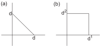
Figure 1: The Newton polytopes of (a) a polynomial with highest total degree $d$. (b) a polynomial with each $x_{a}$ having highest degree $d_{a}$.

There are two operations that can be carried out on polytopes in $\mathbb{R}^{n}$ in order to generate new ones. Let $P,Q$ be polytopes in $\mathbb{R}^{n}$ and let $\lambda\geq 0$ be a real number.

1. The Minkowski sum of $P$ and $Q$ denoted $P+Q$, is

   $$P+Q=\{p+q:p\in P\ {\rm and}\ q\in Q\},$$ (5.44)

   where $p+q$ denotes the usual vector sum in $\mathbb{R}^{n}$

2. The polytope $\lambda P$ is defined by

   $$\lambda P=\{\lambda p:p\in P\},$$ (5.45)

   where $\lambda p$ is the usual scalar multiplication on $\mathbb{R}^{n}$.

We will also define the mixed volume of a collection of polytopes $P_{1},\cdots,P_{n}$, denoted

$$MV_{n}(P_{1},\cdots,P_{n})$$ (5.46)

to be the coefficient of the monomial $\lambda_{1}\lambda_{2}\cdots\lambda_{n}$ in the volume of the polytope $P=\lambda_{1}P_{1}+\cdots+\lambda_{n}P_{n}$.

Using the notions introduced above, we can now write Bernstein’s theorem as follows [32, 33]

Given polynomials $f_{1},\ldots,f_{n}$ over $\mathbb{C}$ with finitely many common zeroes in $(\mathbb{C}^{*})^{n}$, let $P_{i}=NP(f_{i})$ be the Newton polytope of $f_{i}$ in $\mathbb{R}^{n}$. Then the number of common zeros of the $f_{i}$ in $(\mathbb{C}^{*})^{n}$ is bounded above by the mixed volume $MV_{n}(P_{1},\ldots,P_{n})$. Moreover, for generic choices of the coefficients in the $f_{i}$, the number of common solutions is exactly $MV_{n}(P_{1},\ldots,P_{n})$.

For the two cases in $\mathbb{R}^{2}$ described in figure 1 it is simple to calculate the mixed volume. Polynomials $f_{1},f_{2}$ with all terms up to order $d_{1},d_{2}$ have triangular Newton polytopes, as in figure 1(a), and their mixed volume is given by

$$MV_{n}(P_{1},P_{2})=d_{1}d_{2},$$ (5.47)

while polynomials with terms up to order $d_{i}^{1}$ in $x_{1}$ and $d_{i}^{2}$ in $x_{2}$ have square Newton polytopes as in figure 1(b), for which

$$MV_{n}(P_{1},P_{2})=d_{1}^{1}d_{2}^{2}+d_{1}^{2}d_{2}^{1}.$$ (5.48)

5.2.2 The Branches of Moduli Space

Next we will use Bernstein’s theorem to calculate the properties of the moduli space for a generic D4-brane (or several D4-branes) wrapping a 2-cycle on the compact space. We have seen that the supersymmetry condition requires the embedding of the D4-brane to be holomorphic, so the 2-cycle is given by a set of two holomorphic equations in the $z_{i}$. Since the $z_{i}$ are doubly periodic the holomorphic equations should be periodic as well. The most general elliptic function over a torus with complex structure $\tau$ can be written in terms of the periodic Weierstrass functions $w_{i}\equiv\wp(z_{i}|\tau)$ and their derivatives $w_{i}^{\prime}\equiv\wp^{\prime}(z_{i}|\tau)$. For the purposes of Berenstein’s theorem we will treat these variables as independent and add to the set of polynomials $f_{i}$ the relations

$$w_{i}^{\prime 2}-(4w_{i}^{3}+g_{2}(\tau)w_{i}+g_{3}(\tau))=0,\ \ \ i=1,2,3.$$ (5.49)

A general supersymmetric D-brane will thus be located at the zeros of (5.49) and of two holomorphic polynomials of the form

$$P(w_{i},w_{i}^{\prime})=Q(w_{i},w_{i}^{\prime})=0.$$ (5.50)

We can restrict the polynomials to have terms only up to first order in $w_{i}^{\prime}$, since higher powers can be removed using the relations (5.49). We will take the highest degree of the variable $w_{i}$ in $P$ and $Q$ to be $p_{i},q_{i}$, respectively.

Given a set of such polynomials, which describe a D4-brane, we will use Bernstein’s theorem, applied to subsets of this set, to count the wrapping number of the D-brane on the different cycles. Consider for example $N_{1}$ – the number of times the brane wraps the $z_{1}$ cycle. We will evaluate $N_{1}$ by fixing a value of $z_{1}$ and then counting how many solutions there are to the equations for this $z_{1}$ (for a generic $z_{1}$). Fixing $z_{1}$ means that we fix both $w_{1}$ and $w_{1}^{\prime}$ which satisfy the constraint (5.49) for $i=1$. This leaves us with 4 polynomials in the variables $w_{2},w_{3},{w^{\prime}}_{2},{w^{\prime}}_{3}$, on which we apply Bernstein’s theorem. The number of solutions to these equations is

$$N_{1}\sim p_{2}q_{3}+p_{3}q_{2},$$ (5.51)

and similarly for permutations of $\{1,2,3\}$.

Recall that we fix $N_{1,2,3}$ and count the dimensionality of the moduli space for this set of $N$’s. We are interested in finding the values of $p_{i}$ and $q_{i}$ for which we obtain the largest dimensionality. The dimension of the moduli space for a given set of $p_{i}$ and $q_{i}$ can be estimated by the number of different monomials in the two polynomials, which is $8p_{1}p_{2}p_{3}+8q_{1}q_{2}q_{3}$. However, the actual dimension of the moduli space is smaller, since different pairs of polynomials might have the same zero locus. If we assume $q_{i}<p_{i}$, then any multiple of $Q$ with degree smaller than $p_{i}$ can be removed from $P$. We are thus left with a moduli space of dimension

$$D\sim 8(p_{1}p_{2}p_{3}+q_{1}q_{2}q_{3}-(p_{1}-q_{1})(p_{2}-q_{2})(p_{3}-q_{3})).$$ (5.52)

To summarise, we have found that the moduli space describing a domain wall across which the flux jump by $(N_{1},N_{2},N_{3})$ units of flux, consists of different branches each parametrized by a set of 2 polynomials with degrees satisfying (5.51). The dimension of such a branch is given by (5.52).

5.2.3 The Maximal Moduli Space

It is interesting from the point of view of the dual field theory to understand how the dimension of the moduli space scales as we take large wrapping numbers, $N_{i}>>1$ (which should still be much smaller than the fluxes since we are using the probe approximation). For this we will find the dimension of the maximal branch with given wrapping numbers. We can use (5.51) to solve for $q_{i}$ in terms of the $p_{i}$ for given values of the fluxes,

$$q_{1}=\frac{-N_{1}p_{1}+N_{2}p_{2}+N_{3}p_{3}}{2p_{2}p_{3}}$$ (5.53)

and similarly for $q_{2},q_{3}$. Since the $q_{i}$’s are positive, this give some non-trivial condition on the $p_{i}$’s. The requirement $q_{i}<p_{i}$ then leads to the inequalities

$$-N_{1}p_{1}+N_{2}p_{2}+N_{3}p_{3}<2p_{1}p_{2}p_{3},$$ (5.54)

$$N_{1}p_{1}-N_{2}p_{2}+N_{3}p_{3}<2p_{1}p_{2}p_{3},$$ (5.55)

$$N_{1}p_{1}+N_{2}p_{2}-N_{3}p_{3}<2p_{1}p_{2}p_{3},$$ (5.56)

which can be brought to the form

$$N_{1}<2p_{2}p_{3}$$ (5.58)

and its permutations. In the same way we can get $N_{1}>2q_{2}q_{3}$ and its permutations.

We can now use our results in the equation (5.52) for $D$. The term with three $p_{i}$’s cancels. For the terms of the form $ppq$ we can use (5.53) to see that they scale like $N_{i}p_{i}<N_{i}N_{j}$, since $p_{i}$ can be just as large as $N_{j}$ ($j\neq i$). Next, we have $pqq<pN$ so these terms are also smaller than $N_{i}N_{j}$. Finally, the term with three $q_{i}$’s is $qqq<Nq$ and scales as the other terms. Terms with less than three $p$’s or $q$’s are smaller for the same reasons. We thus conclude that for large fluxes the dimension of moduli space behaves as

$$D\leq\sum_{i\neq j}N_{i}N_{j}.$$ (5.59)

We can actually find a configuration which saturates this bound on the dimensionality of moduli space. For instance, if all $N_{i}$ are of the same order, then by choosing all $q_{i}\sim 1$ we get $p_{i}\sim\sum N_{j}$, in which case we get $D\sim\sum_{i\neq j}N_{i}N_{j}$.

The previous analysis was done under the assumption that each $q_{i}$ is smaller than $p_{i}$ so that we can eliminate terms in the polynomial $P$ using $Q$ thus reducing the dimension of moduli space. However it is possible that this is not the case. If one of the $q_{i}$’s is larger we need to take all monomials, and the dimension of the moduli space is $D\sim p_{1}p_{2}p_{3}+q_{1}q_{2}q_{3}$. We will assume that $q_{1}$ is the large $q$ so that $q_{1}>p_{1},q_{2,3}<p_{2,3}$. We find

$$q_{1}>p_{1} \to -N_{1}p_{1}+N_{2}p_{2}+N_{3}p_{3}>2p_{1}p_{2}p_{3},$$ (5.60)

$$q_{2}<p_{2} \to N_{1}q_{1}-N_{2}q_{2}+N_{3}q_{3}>2q_{1}q_{2}q_{3}.$$ (5.61)

From the first inequality we get that $p_{1}p_{2}p_{3}<N_{i}N_{j}$ and from the second one we get that also $q_{1}q_{2}q_{3}<N_{i}N_{j}$ so that we arrive again to the same conclusion (5.59) as before.

In addition to the directions in the moduli space that change the two polynomials and control the embedding of the D-brane, there are additional dimensions of the moduli space related to Wilson lines. The number of Wilson lines is related to the 1 dimensional homology group of the Riemann surface the D-brane is wrapping. We can try to estimate this number as follows. We can think of the polynomials $P(w_{i},w_{i}^{\prime}),Q(w_{i},w_{i}^{\prime})$ as polynomials in a projective space by adding a new variable $\lambda$ and making all terms have the same weight of $p=\sum p_{i}$ and $q=\sum q_{i}$. The relations (5.49) are then of weight $3$. It is then possible using algebraic geometry methods to calculate the Euler characteristic of the complete intersection of these 5 polynomials to be

$$\chi=-27pq(2-p-q).$$ (5.62)

As before, we have $ppq\sim N_{i}p_{j}$ and $qqp\sim N_{i}q_{j}$ so that we have $\chi\sim N_{i}N_{j}$. Since the number of Wilson lines is just the genus, it scales as the Euler characteristic, and we get that

$$D_{Wilson}\sim\sum_{i\neq j}N_{i}N_{j},$$ (5.63)

as before. We thus conclude that the total dimension of the moduli space with given wrapping numbers scales in the same fashion,

$$D_{total}\sim\sum_{i\neq j}N_{i}N_{j}.$$ (5.64)

We note that this behavior may point us towards an $SU(f_{4}^{1})\times SU(f_{4}^{2})\times SU(f_{4}^{3})$ gauge theory, as the dimension of the moduli space can than be viewed as coming from the degrees of freedom of strings sitting in the bifundamental representation of any two $SU(N)$ factors.

Appendix A Supersymmetry Equations in the Bulk

In this appendix we solve the equations for supersymmetry in the bulk for the background discussed in section 2. We find the unbroken spinors and the values for the stabilized moduli.

The equations for preserved supersymmetry are given by [24, 26]

$$e^{-2A+\phi}(d+H\wedge)(e^{2A-\phi}\Psi_{+}) = 2\mu\,\mathcal{R}\mathrm{e}\!\left[\Psi_{-}\right],$$ (A.1)

$$e^{-2A+\phi}(d+H\wedge)(e^{2A-\phi}\Psi_{-}) = 3i\,\mathcal{I}\mathrm{m}\!\left[\bar{\mu}\Psi_{+}\right]+dA\wedge\bar{\Psi}_{-}$$ (A.3)

$$+\frac{\sqrt{2}}{16}e^{\phi}\left[(|a|^{2}-|b|^{2})\hat{F}+i(|a|^{2}+|b|^{2})\tilde{F}\right],$$

where $F=F_{0}+F_{2}+F_{4}+F_{6}$ are the modified RR fields defined as

$$F=e^{-B}F^{\rm bg}+dC+H\wedge C,$$ (A.5)

so that they obey the non-standard Bianchi identity $dF_{n}=-H\wedge F_{n-2}$.

Plugging our background into the first equation we get

$$H\wedge\Psi_{+}=2\mu\,\mathcal{R}\mathrm{e}\!\left[\Psi_{-}\right]$$ (A.6)

$$\Rightarrow-p\beta_{0}\wedge\frac{a\bar{b}}{8}e^{-iJ}=2\mu\,\mathcal{R}\mathrm{e}\!\left[-\frac{iab}{8}\Omega\right]$$ (A.7)

$$\Rightarrow-pa\bar{b}\beta_{0}=2\mu\,\mathcal{I}\mathrm{m}\!\left[ab\Omega\right]=\sqrt{2}\mu\frac{\sqrt{\gamma_{1}\gamma_{2}\gamma_{3}}}{3^{1/4}}(\,\mathcal{R}\mathrm{e}\!\left[ab\right]\beta_{0}+\,\mathcal{I}\mathrm{m}\!\left[ab\right]\alpha_{0}),$$ (A.8)

where $\frac{\sqrt{\gamma_{1}\gamma_{2}\gamma_{3}}}{3^{1/4}\sqrt{2}}\beta_{0}=\,\mathcal{I}\mathrm{m}\!\left[\Omega\right]$ and $\frac{\sqrt{\gamma_{1}\gamma_{2}\gamma_{3}}}{3^{1/4}\sqrt{2}}\alpha_{0}=\,\mathcal{R}\mathrm{e}\!\left[\Omega\right]$. The solution is $\,\mathcal{I}\mathrm{m}\!\left[ab\right]=0$ and

$$-pa\bar{b} = \sqrt{2}\mu\frac{\sqrt{\gamma_{1}\gamma_{2}\gamma_{3}}}{3^{1/4}}ab\Rightarrow$$ (A.10)

$$\mu = -\frac{p}{\sqrt{2}}\frac{3^{1/4}}{\sqrt{\gamma_{1}\gamma_{2}\gamma_{3}}}\frac{\bar{b}}{b}\Rightarrow\Lambda=-|\mu|^{2}=\frac{p^{2}}{2}\frac{\sqrt{3}}{\gamma_{1}\gamma_{2}\gamma_{3}}.$$ (A.11)

In the second equation we use for the left hand side

$$H\wedge\Psi_{-}=-p\beta_{0}\wedge\frac{-iab}{8}\frac{\sqrt{\gamma_{1}\gamma_{2}\gamma_{3}}}{3^{1/4}}\frac{1}{\sqrt{2}}(\alpha_{0}+i\beta_{0})=-\frac{ipab}{8\sqrt{2}}\frac{\sqrt{\gamma_{1}\gamma_{2}\gamma_{3}}}{3^{1/4}}\alpha_{0}\wedge\beta_{0}.$$ (A.12)

This equation can be split according to the rank of the forms that appear in it. The zero-form part of the equation is

$$0=3i\,\mathcal{I}\mathrm{m}\!\left[\frac{\bar{\mu}a\bar{b}}{8}\right]+\frac{\sqrt{2}}{16}e^{\phi}\left[(|a|^{2}-|b|^{2})\hat{F}_{0}-i(|a|^{2}+|b|^{2})*_{6}\hat{F}_{6}\right].$$ (A.13)

The first term is proportional to $\,\mathcal{I}\mathrm{m}\!\left[ab\right]$ so it vanishes. The real part implies

$$|a|=|b|,$$ (A.14)

assuming a non-vanishing value for $\hat{F}_{0}$, while the imaginary part of this equation requires $\hat{F}_{6}=0$ which gives, using (A.5),

$$0 = \int\hat{F}_{6}=\int H\wedge C_{3}+\hat{F}_{6}^{\rm bg}-\hat{F}_{4}^{\rm bg}\wedge B+\frac{1}{2}\hat{F}_{2}^{\rm bg}\wedge B\wedge B-\frac{1}{6}F_{0}^{\rm bg}\wedge B\wedge B\wedge B$$ (A.15)

$$= p\xi-e_{0}-e_{i}b_{i}-\frac{1}{2}\kappa b_{i}b_{j}m_{k}+\kappa m_{0}b_{1}b_{2}b_{3},$$ (A.16)

with $\{i,j,k\}$ being summed over all permutations of $\{1,2,3\}$.

The two-form part is

$$0=3i\,\mathcal{I}\mathrm{m}\!\left[\frac{\bar{\mu}a\bar{b}}{8}(-iJ)\right]+\frac{\sqrt{2}}{16}e^{\phi}\left[(|a|^{2}-|b|^{2})\hat{F}_{2}+i(|a|^{2}+|b|^{2})\tilde{F}_{2}\right],$$ (A.17)

with

$$J=\frac{\gamma_{i}}{2}(\kappa\sqrt{3})^{-1/3}\omega_{i},$$ (A.18)

$$\hat{F}_{2}=-m_{i}w_{i}+m_{0}b_{i}w_{i},$$ (A.19)

$$\tilde{F}_{2}=*_{6}\hat{F}_{4}=-\hat{e}_{i}*\tilde{\omega}^{i}=\frac{2\hat{e}_{i}\gamma_{i}^{2}}{\gamma_{1}\gamma_{2}\gamma_{3}}\left(\frac{\sqrt{3}}{\kappa^{2}}\right)^{1/3}\omega_{i},$$ (A.20)

where we used

$$\hat{F}_{4} = \int H\wedge C_{1}+\hat{F}_{4}^{\rm bg}-\hat{F}_{2}^{\rm bg}\wedge B+\frac{1}{2}\hat{F}_{0}^{\rm bg}\wedge B\wedge B$$ (A.21)

$$= (e_{i}+\kappa(m_{j}b_{k}+m_{k}b_{j})-\kappa m_{0}b_{j}b_{k})\tilde{w}^{i}=\hat{e}_{i}\tilde{w}^{i}.$$ (A.22)

Again, (A.17) splits into real and imaginary parts. The real part vanishes since $|a|=|b|$, while the imaginary part reduces to

$$0 = 3i\frac{-\bar{\mu}a\bar{b}}{8}(J)+i\frac{\sqrt{2}}{16}e^{\phi}(|a|^{2}+|b|^{2})\tilde{F}_{2}$$ (A.23)

$$= i\frac{3}{8}\frac{\gamma_{i}}{2}(\kappa\sqrt{3})^{-1/3}\omega_{i}\frac{p}{\sqrt{2}}\frac{3^{1/4}}{\sqrt{\gamma_{1}\gamma_{2}\gamma_{3}}}ab+ie^{\phi}|a|^{2}\frac{2\sqrt{2}\hat{e}_{i}\gamma_{i}^{2}}{8\gamma_{1}\gamma_{2}\gamma_{3}}\left(\frac{\sqrt{3}}{\kappa^{2}}\right)^{1/3}\omega_{i}$$ (A.24)

which gives

$$\frac{e^{-2\phi}\hat{e}_{i}\gamma_{i}}{\sqrt{\prod_{i}e^{-2\phi}\hat{e}_{i}\gamma_{i}}}=-\frac{3^{11/12}}{8}p\kappa^{1/3}\frac{ab}{|a|^{2}}$$ (A.25)

(with no summation over $i$). This can be solved to give

$$e^{-2\phi}\gamma_{i}=\frac{64}{3^{11/6}}\frac{\hat{e}_{1}\hat{e}_{2}\hat{e}_{3}}{\hat{e}_{i}p^{2}\kappa^{2/3}},$$ (A.26)

where we used $\,\mathcal{I}\mathrm{m}\!\left[ab\right]=0$ and $|a|=|b|$ to get $b=\pm a^{*}$ or $ab=\pm|a|^{2}$. We will later see that we must take the minus sign for the background to be supersymmetric.

The 4-form part of the equation is

$$0=3i\,\mathcal{I}\mathrm{m}\!\left[\frac{\bar{\mu}a\bar{b}}{8}\frac{1}{2}(-iJ)^{2}\right]+\frac{\sqrt{2}}{16}e^{\phi}\left[(|a|^{2}-|b|^{2})\hat{F}_{4}+i(|a|^{2}+|b|^{2})\tilde{F}_{4}\right].$$ (A.27)

Just as before, the first term vanishes, and since we have $\tilde{F}_{4}=*\hat{F}_{2}$ we get

$$0=\int_{[w_{i}]}F_{2}=-m_{i}+m_{0}b_{i}\ \Rightarrow\ b_{i}=\frac{m_{i}}{m_{0}}.$$ (A.28)

Plugging this back into (A.21) we get $\hat{e}_{i}=e_{i}+\kappa\frac{m_{i}m_{j}}{m_{0}}$.

Finally, the 6-form part is

$$H\wedge\Psi_{-}=3i\,\mathcal{I}\mathrm{m}\!\left[\frac{\bar{\mu}a\bar{b}}{8}\frac{1}{6}(-iJ)^{3}\right]+\frac{\sqrt{2}}{16}e^{\phi}\left[(|a|^{2}-|b|^{2})\hat{F}_{6}+i(|a|^{2}+|b|^{2})\tilde{F}_{6}\right].$$ (A.29)

We use (A.12) and

$$\tilde{F}_{6}=*_{6}\hat{F}_{0}=-m_{0}*_{6}1$$ (A.30)

$$\frac{1}{6}J^{3}=\frac{i}{8}\Omega\wedge\bar{\Omega}=\frac{1}{8}\frac{\gamma_{1}\gamma_{2}\gamma_{3}}{\sqrt{3}}\alpha_{0}\wedge\beta_{0}=*1$$ (A.31)

to get

$$0 = -H\wedge\Psi_{-}+3i\,\mathcal{I}\mathrm{m}\!\left[\frac{\bar{\mu}a\bar{b}}{8}\frac{1}{6}(-iJ)^{3}\right]+\frac{\sqrt{2}}{16}e^{\phi}\left[(|a|^{2}-|b|^{2})\hat{F}_{6}+i(|a|^{2}+|b|^{2})\tilde{F}_{6}\right]$$ (A.32)

$$= \frac{ipab}{8\sqrt{2}}\frac{\sqrt{\gamma_{1}\gamma_{2}\gamma_{3}}}{3^{1/4}}\alpha_{0}\wedge\beta_{0}+3i\frac{\bar{\mu}a\bar{b}}{8}\frac{1}{8}\frac{\gamma_{1}\gamma_{2}\gamma_{3}}{\sqrt{3}}\alpha_{0}\wedge\beta_{0}-\frac{1}{16}e^{\phi}i2|a|^{2}\sqrt{2}m_{0}\frac{1}{8}\frac{\gamma_{1}\gamma_{2}\gamma_{3}}{\sqrt{3}}\alpha_{0}\wedge\beta_{0}$$ (A.33)

$$= \frac{ipab}{8\sqrt{2}}\frac{\sqrt{\gamma_{1}\gamma_{2}\gamma_{3}}}{3^{1/4}}\alpha_{0}\wedge\beta_{0}-3i\frac{p}{\sqrt{2}}\frac{3^{1/4}}{\sqrt{\gamma_{1}\gamma_{2}\gamma_{3}}}\frac{ab}{8}\frac{1}{8}\frac{\gamma_{1}\gamma_{2}\gamma_{3}}{\sqrt{3}}\alpha_{0}\wedge\beta_{0}$$ (A.35)

$$-\frac{1}{16}e^{\phi}i2|a|^{2}\sqrt{2}m_{0}\frac{1}{8}\frac{\gamma_{1}\gamma_{2}\gamma_{3}}{\sqrt{3}}\alpha_{0}\wedge\beta_{0}$$

$$= \frac{5}{8}\frac{ipab}{8\sqrt{2}}\frac{\sqrt{\gamma_{1}\gamma_{2}\gamma_{3}}}{3^{1/4}}\alpha_{0}\wedge\beta_{0}-\frac{1}{16}e^{\phi}i2|a|^{2}\sqrt{2}m_{0}\frac{1}{8}\frac{\gamma_{1}\gamma_{2}\gamma_{3}}{\sqrt{3}}\alpha_{0}\wedge\beta_{0},$$ (A.36)

which gives us

$$e^{4\phi}\sqrt{\prod_{i}e^{-2\phi}\gamma_{i}}=\frac{5\cdot 3^{1/4}}{2}\frac{p}{m_{0}}\frac{ab}{|a|^{2}}.$$ (A.37)

Using (A.26) we can solve for $e^{\phi}$ and $\gamma_{i}$. We know that the O6-plane generates a tadpole that is canceled by the fluxes $m_{0}$ and $p$ according to (2.25), so that we find ${\rm sign}(m_{0}p)=-$. We thus must have, for supersymmetry to hold, $b=-a^{*}$ as stated in the main text. The results we got for the moduli agree with (2.26).

We note that equations (A.25), (A.37) give us the following conditions on the signs of the background fluxes,

$${\rm sign}(pe_{i})=+,\quad{\rm sign}(pm_{0})=-.$$ (A.38)

Appendix B BPS Condition

In this appendix we will consider the supersymmetric domain wall solutions found in section 4. Such a supersymmetric configuration should be a BPS state and therefore feel no radial force. We will verify this fact directly by considering the D-brane effective action. (This was independently verified in [26].) In the supersymmetric configuration the gravitational force coming from the DBI term will be canceled against the RR force coming from the WZ term, related to the charge of the D-brane.

The D-branes extend along a $2+1$ dimensional surface in $AdS_{4}$ parallel to the boundary at constant $r$, and wrap a $(p-2)$-cycle in the compact space. Their world-sheet action in the string frame is given by

$$I_{brane}=I_{DBI}+I_{WZ}~{},$$ (B.1)

where

$$I_{DBI}=-\mu_{p}\int d^{p}xe^{-\phi}\sqrt{-\det\left(G+{\cal F}\right)}$$ (B.2)

is a Dirac-Born-Infeld type action in the string frame, $\mu_{p}$ is the D-brane tension and

$${\cal F}=f+P[B]~{}.$$ (B.3)

$I_{WZ}$ is the following Wess-Zumino (WZ) type action

$$I_{WZ}=\sqrt{2}\mu_{p}\int\left({\cal C}\wedge e^{\cal F}+m_{0}\omega\right)~{},$$ (B.4)

where

$${\cal C}=\sum_{i=0}^{9}{\cal C}_{i}~{},\qquad d\omega=e^{{\cal F}}$$ (B.5)

and $m_{0}$ is the massive type IIA mass parameter. The $\sqrt{2}$ is due to the different normalization of the RR fields we use (following [13]).

As in [31], the brane action has two contributions which depend on the radial location of the brane in $AdS_{4}$. One contribution is proportional to the brane area $A$ and comes from the DBI action, the other is proportional to the volume enclosed by the brane $V$ and comes from the WZ action. Next, we are going to evaluate the different terms for wrapped D4-branes. We will assume ${\cal F}=0$.

The $D4$-brane domain walls wrap a two-cycle in the compact space. In our background there is a 3-dimensional basis for the untwisted 2-cycles given by $[\omega_{i}],\ i=1,2,3.$ For simplicity we consider wrapping the two-cycle $[\omega_{1}]$ in $T^{6}/Z_{3}^{2}$.

DBI

In this case we have

$$\sqrt{-\det\ G}=\gamma_{1}du^{1}dv^{1}\frac{r^{3}}{R_{\rm AdS}^{3}}dtdx^{1}dx^{2},$$ (B.6)

so we have

$$I_{\rm DBI}=\mu_{4}\int d^{5}xe^{-\phi}\sqrt{-\det\ G}=\mu_{4}a\gamma_{1}e^{-\phi}{r^{3}\over R_{\rm AdS}^{3}}\int d^{3}x=\mu_{4}3^{-{13\over 12}}2^{\frac{7}{2}}5^{\frac{1}{4}}{\kappa^{\frac{1}{3}}E^{\frac{3}{4}}\over e_{1}pm_{0}^{\frac{1}{4}}}\ {r^{3}\over R_{\rm AdS}^{3}}a\int d^{3}x~{},$$ (B.7)

where we define

$$a\equiv\int_{[\omega_{1}]}du^{1}dv^{1}~{}.$$ (B.8)

WZ

The only non-zero contribution to the WZ term is given by

$$\mu_{4}\sqrt{2}\int_{W_{5}}{\cal C}_{5}=\mu_{4}\sqrt{2}\int_{{\rm Vol}(W_{5})}F_{6},$$ (B.9)

where $W_{5}$ is the D4-brane worldvolume wrapping a 2-cycle in the compact space and spanning a surface of constant $r$ in the AdS space. ${\rm Vol}(W_{5})$ is the two cycle times the volume in AdS bounded by the surface of constant $r$. The other boundary of the volume, at $r\to\infty$, gives a contribution $\sim r^{-3}\to 0$ so it does not contribute.

The supergravity fields obey

$$\tilde{F}_{6}\equiv*\tilde{F}_{4}=F_{6}-C_{3}\wedge H_{3}+\frac{m_{0}}{6}B_{2}\wedge B_{2}\wedge B_{2}.$$ (B.10)

Integrating over ${\rm Vol}(W_{5})$ we get that the last two terms vanish, since there are no such background fields with indices in the non-compact space. We can then write

$$\int_{{\rm Vol}(W_{5})}*\tilde{F}_{4}=\int_{{\rm Vol}(W_{5})}F_{6}.$$ (B.11)

The right-hand side is what we want to calculate, while the left-hand side is proportional to the integration of $\tilde{F}_{4}$ over the dual cycle which we can calculate.

In massive type IIA supergravity we have

$$\tilde{F}_{4} =dC_{3}+F_{4}^{bg}-C_{1}\wedge H_{3}-\frac{m_{0}}{2}B_{2}\wedge B_{2}.$$ (B.12)

since the $B_{2}$ and $C_{1}$ are only the fluctuations and vanish in the background, we can replace $\tilde{F}_{4}$ in the integral by $F_{4}$.

In addition to a boundary term we are left with

$$\int_{w_{2}\times w_{3}}\tilde{F}_{4}=\int_{w_{2}\times w_{3}}F_{4}^{\rm bg},$$ (B.13)

and the WZ term can now be written as

$$\mu_{4}\sqrt{2}\int_{{\rm Vol}(W_{5})}*F_{4}.$$ (B.14)

Now

$$F_{4} = e_{i}\tilde{\omega}^{i}=-\left({3\over\kappa}\right)^{\frac{1}{3}}e_{1}(dz^{2}\wedge d\bar{z}^{2})\wedge(dz^{3}\wedge d\bar{z}^{3})+\dots,$$ (B.15)

$$\ast F_{4} = -4\left({3\over\kappa}\right)^{\frac{1}{3}}e_{1}{\gamma_{1}\over\gamma_{2}\gamma_{3}}\Omega_{AdS_{4}}\wedge(du^{1}\wedge dv^{1})+\dots~{}$$ (B.16)

$$= -2e_{i}\gamma_{i}\frac{\gamma_{i}}{\gamma_{1}\gamma_{2}\gamma_{3}}\left(\frac{\sqrt{3}}{\kappa^{2}}\right)^{1/3}\omega_{i},$$ (B.17)

where $\Omega_{AdS_{4}}$ is the volume form in $AdS$. We find

$$I_{\rm WZ} = \mu_{4}\sqrt{2}\int_{W}{{\cal C}_{5}}=-\mu_{4}4\sqrt{2}\left(3\over\kappa\right)^{\frac{1}{3}}{a\over 2\kappa^{\frac{1}{3}}3^{\frac{1}{6}}}{e_{1}v_{1}\over v_{2}v_{3}}{r^{3}\over R_{AdS}^{4}}\int d^{3}x$$ (B.18)

$$= -\mu_{4}3^{-{13\over 12}}2^{\frac{7}{2}}5^{\frac{1}{4}}{\kappa^{\frac{1}{3}}E^{\frac{3}{4}}\over e_{1}pm_{0}^{\frac{1}{4}}}\ {r^{3}\over R_{\rm AdS}^{3}}a\int d^{3}x=-I_{DBI}.$$ (B.19)

Thus, the gravitational force due to the DBI term is canceled exactly by the force from the WZ term, as must be the case for a BPS configuration.

The analysis is very similar for a more general cycle, and we will not write it down explicitly here.

Appendix C Other Domain Walls

Here we consider D2 and D6-branes in domain wall configurations and study their supersymmetry equations. We show that a D2-brane can never be supersymmetric. A D6-brane can classically be supersymmetric, however due to flux quantization there are generically no such solutions with integer values for the flux.

C.1    D2-Brane as a Supersymmetric Domain Wall

The $\kappa$-symmetry equation (4.1) takes a simple form when we consider D2-branes, since they are not extended along any compact dimension. In order for these domain walls to be supersymmetric we need

$$\gamma_{\underline{012}}\epsilon_{-}=\epsilon_{+}.$$ (C.1)

This can be brought to the form

$$\gamma_{\underline{012}}\theta_{+}\otimes b^{*}\eta_{-}=\theta_{-}\otimes a^{*}\eta_{-}.$$ (C.2)

The $AdS_{4}$ part of the equation is the same as for D4-branes, which results in the equation

$$b^{*}=\alpha a^{*}=-{\rm sign}(p)i\frac{b^{*}}{b}a^{*}\quad\to\quad b=-{\rm sign}(p)ia^{*},$$ (C.3)

which contradicts our supersymmetric condition in the bulk, $b=-a^{*}$. Therefore we conclude that D2-branes cannot be supersymmetric domain walls in this background.

C.2    D6-Brane as a Supersymmetric Domain Wall

Consider now a D6-brane which extends as a domain wall in the AdS and wraps (for instance) the 4-torus spanned by $z_{1},z_{2}$. Its embedding may be chosen as

$$\sigma^{1}=x^{1},\quad\sigma^{2}=y^{1},\qquad\sigma^{3}=x^{2},\quad\sigma^{4}=y^{2},$$ (C.4)

with the induced metric being

$$\gamma_{1}(d\sigma^{1})^{2}+\gamma_{1}(d\sigma^{2})^{2}+\gamma_{2}(d\sigma^{3})^{2}+\gamma_{2}(d\sigma^{4})^{2},$$ (C.5)

and the pullback of $J$ given by

$$P[J]=\gamma_{1}d\sigma^{1}\wedge d\sigma^{2}+\gamma_{2}d\sigma^{3}\wedge d\sigma^{4}.$$ (C.6)

Plugging into the supersymmetry condition (4.7) and taking ${\cal F}=0$ as for the D4-branes, we have on the right-hand side

$$-a^{*}\alpha\sqrt{\det(P[g]+{\cal F})}d\sigma^{1}\wedge d\sigma^{2}\wedge d\sigma^{3}\wedge d\sigma^{4}=-{\rm sign}(p)ib^{*}\gamma_{1}\gamma_{2}d\sigma^{1}\wedge d\sigma^{2}\wedge d\sigma^{3}\wedge d\sigma^{4}$$ (C.7)

while on the left-hand side we have

$$\{b^{*}P[e^{-iJ}])\wedge e^{\cal F}\}_{4}=b^{*}\frac{1}{2}(-iP[J])\wedge(-iP[J])=b^{*}\frac{1}{2}(P[J])\wedge(P[J]))$$ (C.8)

$$=b^{*}\gamma_{1}\gamma_{2}d\sigma^{1}\wedge d\sigma^{2}\wedge d\sigma^{3}\wedge d\sigma^{4}.$$ (C.9)

Since the first is purely imaginary and the second is real they cannot be equal, and the domain walls are not supersymmetric. A more generic embedding will not be able to compensate for the factor of $i$, and so even the general case is not supersymmetric. However as we have seen for the D4-branes, adding non trivial ${\cal F}$ can add a relative phase between the two sides. With ${\cal F}=f_{1}d\sigma^{1}\wedge d\sigma^{2}+f_{2}d\sigma^{3}\wedge d\sigma^{4}$ the $\kappa$-symmetry equation becomes

$$b^{*}(f_{1}-i\gamma_{1})(f_{2}-i\gamma_{2})=-{\rm sign}(p)ib^{*}\sqrt{(\gamma_{1}^{2}+f_{1}^{2})(\gamma_{2}^{2}+f_{2}^{2})}.$$ (C.10)

Writing $f-i\gamma=\sqrt{f^{2}+\gamma^{2}}e^{-\tan^{-1}(\gamma/f)}$ we get that for positive $p$

$$\tan^{-1}(\gamma_{1}/f_{1})+\tan^{-1}(\gamma_{2}/f_{2})=\pi/2$$ (C.11)

which has a solution for $f_{i}>0$. For negative $p$ the right hand side should be $3\pi/4$ so there are solutions for $f_{i}>-\gamma_{i}$. Classically such supersymmetric configurations exist, however generically there are no such configurations consistent with flux quantization.

References

- [1] A. R. Frey, “Warped strings: Self-dual flux and contemporary compactifications,” arXiv:hep-th/0308156.
- [2] E. Silverstein, “TASI / PiTP / ISS lectures on moduli and microphysics,” arXiv:hep-th/0405068.
- [3] M. Grana, “Flux compactifications in string theory: A comprehensive review,” Phys. Rept. 423, 91 (2006) [arXiv:hep-th/0509003].
- [4] J. Polchinski, “The cosmological constant and the string landscape,” arXiv:hep-th/0603249.
- [5] M. R. Douglas and S. Kachru, “Flux compactification,” Rev. Mod. Phys. 79, 733 (2007) [arXiv:hep-th/0610102].
- [6] F. Denef, M. R. Douglas and S. Kachru, “Physics of string flux compactifications,” Ann. Rev. Nucl. Part. Sci. 57, 119 (2007) [arXiv:hep-th/0701050].
- [7] T. Banks, “Landskepticism or why effective potentials don’t count string models,” arXiv:hep-th/0412129.
- [8] J. M. Maldacena, “The large N limit of superconformal field theories and supergravity,” Adv. Theor. Math. Phys. 2, 231 (1998) [Int. J. Theor. Phys. 38, 1113 (1999)] [arXiv:hep-th/9711200].
- [9] E. Witten, “Anti-de Sitter space and holography,” Adv. Theor. Math. Phys. 2, 253 (1998) [arXiv:hep-th/9802150].
- [10] S. S. Gubser, I. R. Klebanov and A. M. Polyakov, “Gauge theory correlators from non-critical string theory,” Phys. Lett. B 428, 105 (1998) [arXiv:hep-th/9802109].
- [11] M. Fabinger and E. Silverstein, “D-Sitter space: Causal structure, thermodynamics, and entropy,” JHEP 0412 (2004) 061 [arXiv:hep-th/0304220].
- [12] E. Silverstein, “AdS and dS entropy from string junctions or the function of junction conjunctions,” arXiv:hep-th/0308175.
- [13] O. DeWolfe, A. Giryavets, S. Kachru and W. Taylor, “Type IIA moduli stabilization,” JHEP 0507, 066 (2005) [arXiv:hep-th/0505160].
- [14] D. Lust and D. Tsimpis, “Supersymmetric AdS(4) compactifications of IIA supergravity,” JHEP 0502, 027 (2005) [arXiv:hep-th/0412250].
- [15] B. S. Acharya, F. Benini and R. Valandro, “Fixing moduli in exact type IIA flux vacua,” JHEP 0702 (2007) 018 [arXiv:hep-th/0607223].
- [16] T. Banks and K. van den Broek, “Massive IIA flux compactifications and U-dualities,” JHEP 0703 (2007) 068 [arXiv:hep-th/0611185].
- [17] C. Kounnas, D. Lust, P. M. Petropoulos and D. Tsimpis, “AdS4 flux vacua in type II superstrings and their domain-wall solutions,” JHEP 0709, 051 (2007) [arXiv:0707.4270 [hep-th]].
- [18] L. J. Dixon, J. A. Harvey, C. Vafa and E. Witten, “Strings On Orbifolds,” Nucl. Phys. B 261, 678 (1985).
- [19] A. Strominger, “Topology Of Superstring Compactification,” NSF-ITP-85-109 Presented at Santa Barbara Workshop on Unified String Theories, Santa Barbara, CA, Jul 29 - Aug 16, 1985
- [20] R. Blumenhagen, L. Gorlich and B. Kors, “Supersymmetric 4D orientifolds of type IIA with D6-branes at angles,” JHEP 0001, 040 (2000) [arXiv:hep-th/9912204].
- [21] L. J. Romans, “Massive N=2a Supergravity In Ten-Dimensions,” Phys. Lett. B 169, 374 (1986).
- [22] T. W. Grimm and J. Louis, “The effective action of type IIA Calabi-Yau orientifolds,” Nucl. Phys. B 718, 153 (2005) [arXiv:hep-th/0412277].
- [23] M. Grana, R. Minasian, M. Petrini and A. Tomasiello, “Supersymmetric backgrounds from generalized Calabi-Yau manifolds,” JHEP 0408, 046 (2004) [arXiv:hep-th/0406137].
- [24] M. Grana, R. Minasian, M. Petrini and A. Tomasiello, “Generalized structures of N=1 vacua,” JHEP 0511, 020 (2005) [arXiv:hep-th/0505212].
- [25] L. Martucci and P. Smyth, “Supersymmetric D-branes and calibrations on general N = 1 backgrounds,” JHEP 0511, 048 (2005) [arXiv:hep-th/0507099].
- [26] P. Koerber and L. Martucci, “D-branes on AdS flux compactifications,” JHEP 0801, 047 (2008) [arXiv:0710.5530 [hep-th]].
- [27] P. Koerber, “Stable D-branes, calibrations and generalized Calabi-Yau geometry,” JHEP 0508, 099 (2005) [arXiv:hep-th/0506154].
- [28] E. Bergshoeff and P. K. Townsend, “Super D-branes,” Nucl. Phys. B 490, 145 (1997) [arXiv:hep-th/9611173].
- [29] H. Lu, C. N. Pope and P. K. Townsend, “Domain walls from anti-de Sitter spacetime,” Phys. Lett. B 391, 39 (1997) [arXiv:hep-th/9607164].
- [30] H. Lu, C. N. Pope and J. Rahmfeld, “A construction of Killing spinors on S**n,” J. Math. Phys. 40, 4518 (1999) [arXiv:hep-th/9805151].
- [31] N. Seiberg and E. Witten, “The D1/D5 system and singular CFT,” JHEP 9904, 017 (1999) [arXiv:hep-th/9903224].
- [32] David Cox, John Little, Donal O’shea, Using Algebraic Geometry (Graduate Texts in Mathematics).
- [33] D. Bernstein, ”The number of roots of a system of equations,” Functional Anal. Appl. 9 (1975), 1-4.