Tachyon-Chaplygin inflationary universe model

Abstract

Tachyonic inflationary universe model in the context of a Chaplygin gas equation of state is studied. General conditions for this model to be realizable are discussed. By using an effective exponential potential we describe in great details the characteristic of the inflationary universe model. The parameters of the model are restricted by using recent astronomical observations.

I Introduction

It is well known that inflation is to date the most compelling solution to many long-standing problems of the Big Bang model (horizon, flatness, monopoles, etc.) guth ; infla . One of the success of the inflationary universe model is that it provides a causal interpretation of the origin of the observed anisotropy of the cosmic microwave background (CMB) radiation, and also the distribution of large scale structures astro .

In concern to higher dimensional theories, implications of string/M-theory to Friedmann-Robertson-Walker (FRW) cosmological models have recently attracted great deal of attention, in particular, those related to brane-antibrane configurations such as space-like branessen1 . In recent times a great amount of work has been invested in studying the inflationary model with a tachyon field. The tachyon field associated with unstable D-branes might be responsible for cosmological inflation in the early evolution of the universe, due to tachyon condensation near the top of the effective scalar potential sen2 , which could also add some new form of cosmological dark matter at late times Sami_taq . In fact, historically, as was empathized by Gibbons gibbons , if the tachyon condensate starts to roll down the potential with small initial velocity, then a universe dominated by this new form of matter will smoothly evolve from a phase of accelerated expansion (inflation) to an era dominated by a non-relativistic fluid, which could contribute to the dark matter detected in these days.

On the other hand, the generalized Chaplygin gas has been proposed as an alternative model for describing the accelerating of the universe. The generalized Chaplygin gas is described by an exotic equation of state of the form Bento

$$p_{ch}=-\frac{A}{\rho_{ch}^{\beta}},$$ (1)

where $\rho_{ch}$ and $p_{ch}$ are the energy density and pressure of the generalized Chaplygin gas, respectively. $\beta$ is a constant that lies in the range $0<\beta\leq 1$, and $A$ is a positive constant. The original Chaplygin gas corresponds to the case $\beta=1$ 2 . Inserting this equation of state into the relativistic energy conservation equation leads to an energy density given by Bento

$$\rho_{ch}=\left[A+\frac{B}{a^{3(1+\beta)}}\right]^{\frac{1}{1+\beta}},$$ (2)

where $a$ is the scale factor and $B$ is a positive integration constant.

The Chaplygin gas emerges as a effective fluid of a generalized d-brane in a (d+1, 1) space time, where the action can be written as a generalized Born-Infeld action Bento . These models have been extensively studied in the literature other . The model parameters were constrained using currents cosmological observations, such as, CMB CMB and supernova of type Ia (SNIa) SIa .

In the model of Chaplygin inspired inflation usually the scalar field, which drives inflation, is the standard inflaton field, where the energy density given by Eq.(2), can be extrapolate for obtaining a successful inflation period with a Chaplygin gas modelIc . Recently, the dynamics of the early universe and the initial conditions for inflation in a model with radiation and a Chaplygin gas was studied in Ref.Monerat:2007ud . As far as we know, a Chaplygin inspired inflationary model in which a tachyonic field is considered has not been studied. The main goal of the present work is to investigate the possible realization of a Chaplygin inflationary universe model, where the energy density is driven by a tachyonic field. We use astronomical data for constraining the parameters appearing in this model.

The outline of the paper is a follows. The next section presents a short review of the modified Friedmann equation by using a Chaplygin gas, and we present the tachyon-Chaplygin inflationary model. Section III deals with the calculations of cosmological perturbations in general term. In Section IV we use an exponential potential for obtaining explicit expression for the model. Finally, Sect.V summarizes our findings.

II The modified Friedmann equation and the Tachyon-Chaplygin Inflationary phase.

We start by writing down the modified Friedmann equation, by using the FRW metric. In particular, we assume that the gravitational dynamics give rise to a modified Friedmann equation of form

$$H^{2}=\kappa\left[A+\rho_{\phi}^{(1+\beta)}\right]^{\frac{1}{1+\beta}},$$ (3)

where $\kappa=8\pi G/3=8\pi/3m_{p}^{2}$ (here $m_{p}$ represents the Planck mass), $\rho_{\phi}=\frac{V(\phi)}{\sqrt{1-\dot{\phi}^{2}}}$, and $V(\phi)=V$ is the scalar tachyonic potential. The modification is realized from an extrapolation of Eq.(2), where the density matter $\rho_{m}\sim a^{-3}$ in introduced in such a way that we may write

$$\rho_{ch}=\left[A+\rho_{m}^{(1+\beta)}\right]^{\frac{1}{1+\beta}},$$ (4)

and thus, we identifying $\rho_{m}$ with the contributions of the tachyon field for give Eq.(3). The generalized Chaplygin gas model may be viewed as a modification of gravity, as described in Ref.Ber , and for chaotic inflation, in Ref.Ic . Different modifications of gravity have been proposed in the last few years, and there has been a lot of interest in the construction of early universe scenarios in higher-dimensional models motivated by string/M-theory Ran . It is well-known that these modifications can lead to important changes in the early universe. In the following we will take $\beta=1$ for simplicity, which means the usual Chaplygin gas.

From Eq.(3), the dynamics of the cosmological model in the tachyon-Chaplygin inflationary scenario is described by the equations

$$H^{2}=\kappa\,\sqrt{A+\rho_{\phi}^{2}}=\kappa\,\sqrt{A+\frac{V^{2}}{1-\dot{\phi}^{2}}},$$ (5)

and

$$\frac{\ddot{\phi}}{1-\dot{\phi}^{2}}+\,3H\;\dot{\phi}+\frac{V^{\prime}}{V}=0,$$ (6)

where dots mean derivatives with respect to the cosmological time and $V^{\prime}=\partial V(\phi)/\partial\phi$. For convenience we will use units in which $c=\hbar=1$.

During the inflationary epoch the energy density associated to the tachyon field is of the order of the potential, i.e. $\rho_{\phi}\sim V$. Assuming the set of slow-roll conditions, i.e. $\dot{\phi}^{2}\ll 1$ and $\ddot{\phi}\ll 3H\dot{\phi}$ gibbons ; Fairbairn:2002yp , the Friedmann equation (5) reduces to

$$H^{2}=\kappa\,\sqrt{A+\rho_{\phi}^{2}}\approx\kappa\,\sqrt{A+V^{2}},$$ (7)

and Eq. (6) becomes

$$3H\dot{\phi}\approx-\frac{V^{\prime}}{V}.$$ (8)

Introducing the dimensionless slow-roll parameters Hwang:2002fp , we write

$$\varepsilon=-\frac{\dot{H}}{H^{2}}\simeq\frac{1}{6\kappa}\,\frac{V^{\prime 2}}{(A+V^{2})^{3/2}},$$ (9)

$$\eta=-\frac{\ddot{\phi}}{H\,\dot{\phi}}\simeq\,\frac{1}{3\kappa\sqrt{A+V^{2}}}\left[\frac{V^{\prime\prime}}{V}-\frac{V^{\prime 2}}{V^{2}}-\frac{1}{2}\frac{V^{\prime 2}}{(A+V^{2})}\right],$$ (10)

and

$$\gamma=-\frac{V^{\prime}\,\dot{\phi}}{2\,H\,V}\simeq\frac{1}{6\kappa}\,\frac{V^{\prime 2}}{V^{2}\,(A+V^{2})^{1/2}}.$$ (11)

The condition under which inflation takes place can be summarized with the parameter $\varepsilon$ satisfying the inequality $\varepsilon<1.$, which is analogue to the requirement that $\ddot{a}>0$. This condition could be written in terms of the tachyon potential and its derivative $V^{\prime}$, which becomes

$$(A+V^{2})^{3/2}>\frac{V^{\prime 2}}{6\kappa}.$$ (12)

Inflation ends when the universe heats up at a time when $\varepsilon\simeq 1$, which implies

$$(A+V_{f}^{2})^{3/2}\simeq\frac{V_{f}^{\prime}\,{}^{2}}{6\kappa}.$$ (13)

The number of e-folds at the end of inflation is given by

$$N=-3\;\kappa\,\int_{\phi_{*}}^{\phi_{f}}\frac{\sqrt{A+V^{2}}}{V^{\prime}}\,V\,d\phi^{\prime},$$ (14)

or equivalently

$$N=-3\;\kappa\,\int_{V_{*}}^{V_{f}}\frac{\sqrt{A+V^{2}}}{V^{\prime 2}}\,V\,d\,V.$$ (15)

In the following, the subscripts $*$ and $f$ are used to denote the epoch when the cosmological scales exit the horizon and the end of inflation, respectively.

III Perturbations

In this section we will study the scalar and tensor perturbations for our model. The general perturbed metric about the flat FRW background Bar is :

$$ds^{2}=-(1+2A)dt^{2}+2a(t)B_{,\,i}dx^{i}dt+a(t)^{2}[(1-2\psi)\delta_{ij}+2E_{,\,i,\,j}+2h_{ij}]dx^{i}dx^{j}\,,$$ (16)

where $A$, $B$, $\psi$ and $E$ correspond to the scalar-type metric perturbations, and $h_{ij}$ characterizes the transverse-traceless tensor-type perturbation. We introduce comoving curvature perturbations, $\cal{R}=\psi+H\delta\phi/\dot{\phi}$, where $\delta\phi$ is the perturbation of the scalar field $\phi$. For a tachyon field the power spectrum of the curvature perturbations is given in the slow-roll approximation by following expression Hwang:2002fp

$${\cal{P}_{R}}\simeq\left(\frac{H^{2}}{2\pi\dot{\phi}}\right)^{2}\,\frac{1}{V}\simeq\frac{9\kappa^{3}}{4\pi^{2}}\,\left[\frac{V\,(A+V^{2})^{3/2}}{V^{\prime 2}}\right].$$ (17)

The scalar spectral index $n_{s}$ is given by $n_{s}-1=\frac{d\ln\,{\cal{P}_{R}}}{d\ln k}$, where the interval in wave number is related to the number of e-folds by the relation $d\ln k(\phi)=-dN(\phi)$. From Eq.(17), we get, by using the slow-roll parameters,

$$n_{s}\approx\,1\,-2(2\varepsilon-\eta-\gamma),$$ (18)

or equivalently

$$n_{s}\approx\,1\,-\frac{1}{\kappa\,(A+V^{2})^{1/2}}\,\left[\frac{V^{\prime 2}}{(A+V^{2})}+\frac{V^{\prime 2}}{3\,V^{2}}-\frac{2}{3}\frac{V^{\prime\prime}}{V}\right].$$ (19)

Note that in the limit $A\rightarrow 0$, the scalar spectral index $n_{s}$ coincides with that corresponding to a single tachyon field Sami_taq .

One of the interesting features of the three-year data set from Wilkinson Microwave Anisotropy Probe (WMAP) is that it hints at a significant running in the scalar spectral index $dn_{s}/d\ln k=\alpha_{s}$ astro . From Eq.(18) we get that the running of the scalar spectral index becomes

$$\alpha_{s}=\left(\frac{4\,(A+V^{2})}{V\;V^{\prime}}\right)\,[2\varepsilon_{,\,\phi}-\eta_{,\,\phi}-\gamma_{,\,\phi}]\;\varepsilon.$$ (20)

In models with only scalar fluctuations the marginalized value for the derivative of the spectral index is approximately $-0.05$ from WMAP-three year data only astro .

On the other hand, the generation of tensor perturbations during inflation would produce gravitational waves and its amplitudes are given by Bar

$${\cal{P}}_{g}=24\kappa\,\left(\frac{H}{2\pi}\right)^{2}\simeq\frac{6}{\pi^{2}}\,\kappa^{2}\,(A+V^{2})^{1/2},$$ (21)

where the spectral index $n_{g}$ is given by $n_{g}=\frac{d{\cal{P}}_{g}}{d\,\ln k}=-2\,\varepsilon$.

From expressions (17) and (21) we write the tensor-scalar ratio as

$$R(k)=\left.\left(\frac{{\cal{P}}_{g}}{P_{\cal R}}\right)\right|_{k=k_{*}}\simeq\left.\left(\frac{24\kappa\,V\,\dot{\phi}^{2}}{H^{2}}\right)\right|_{\,k=k_{*}}=\left.\left(\frac{8}{3\,\kappa}\,\frac{V^{\prime 2}}{V\;(A+V^{2})}\right)\right|_{\,k=k_{*}}.$$ (22)

Here, $k_{*}$ is referred to $k=Ha$, the value when the universe scale crosses the Hubble horizon during inflation. Note that the consistency relation for the tensor-scalar ratio, $R=-8\,n_{g}$, becomes similar to that corresponding to the standard scalar field Steer:2003yu .

Combining WMAP three-year dataastro with the Sloan Digital Sky Survey (SDSS) large scale structure surveys Teg , it is found an upper bound for $R$ given by $R(k_{*}\simeq$ 0.002 Mpc^-1)$<0.28\,(95\%CL)$, where $k_{*}\simeq$0.002 Mpc^-1 corresponds to $l=\tau_{0}k\simeq 30$, with the distance to the decoupling surface $\tau_{0}$= 14,400 Mpc. The SDSS measures galaxy distributions at red-shifts $a\sim 0.1$ and probes $k$ in the range 0.016 $h$ Mpc^-1$<k<$0.011 $h$ Mpc^-1. The recent WMAP three-year results give the values for the scalar curvature spectrum $P_{\cal R}(k_{*})\simeq 2.3\times\,10^{-9}$ and the scalar-tensor ratio $R(k_{*})=0.095$. We will make use of these values to set constrains on the parameters appearing in our model.

IV Exponential potential in a Tachyon-Chaplygin gas.

Let us consider a tachyonic effective potential $V(\phi)$, with the properties satisfying $V(\phi)\longrightarrow$ 0 as $\phi\longrightarrow\infty$. The exact form of the potential is $V(\phi)=\left(1+\alpha\phi\right)\exp(-\alpha\phi)$, which in the case when $\alpha\rightarrow 0$, we may use the asymptotic exponential expression. This form for the potential is derived from string theory calculationsku ; sen2 . Therefore, we simple use

$$V(\phi)=V_{0}e^{-\alpha\phi},$$ (23)

where $\alpha$ and $V_{0}$ are free parameters. In the following we will restrict ourselves to the case in which $\alpha>0$. Note that $\alpha$ represents the tachyon mass Fairbairn:2002yp ; delaMacorra:2006tm . In Ref.Sami_taq is given an estimation of these parameters in the limit $A\rightarrow 0$. Here, it was found $V_{0}\sim 10^{-10}m_{p}^{4}$ and $\alpha\sim 10^{-6}m_{p}$. We should mention here that the caustic problem with multi-valued regions for scalar Born-Infeld theories with an exponential potential results in high order spatial derivatives of the tachyon field, $\phi$, become divergentko .

From Eq.(15) the number of e-folds results in

$$N=\frac{3\kappa}{\alpha^{2}}\;[h(V_{f})-h(V_{*})],$$ (24)

where

$$h(V)=\left(\sqrt{A}\;\ln\left[\frac{2(\sqrt{A}+W)}{A\,V}\right]-W\right),$$ (25)

and $W=W(V)=(A+V^{2})^{1/2}$.

On the other hand, we may establish that the end of inflation is governed by the condition $\varepsilon=1$, from which we get that the square of the scalar tachyon potential becomes

$$V^{2}(\phi=\phi_{f})=V_{f}^{2}=\frac{1}{108\kappa^{2}}\,\left[\alpha^{4}-108\,A\,\kappa^{2}+\frac{\alpha^{8}-216\,A\,\kappa^{2}\,\alpha^{4}}{\Im}+\Im\right].$$ (26)

Here, $\Im$ is given by

$$\Im=\alpha^{4/3}\;[\alpha^{8}-324\,A\kappa^{2}\alpha^{4}+17496\,A^{2}\,\kappa^{4}\,+648\sqrt{3}\,A^{3/2}\kappa^{3}\,\sqrt{243A\kappa^{2}-\alpha^{4}}\,]^{1/3}.$$

Note that in the limit $A\rightarrow 0$ we obtain $V_{f}=\frac{\alpha^{2}}{6\kappa}$, which coincides with that reported in Ref.Sami_taq .

From Eq.(17) we obtain that the scalar power spectrum is given by

$$P_{\cal R}(k)\approx\left.\;\frac{9\kappa^{3}}{4\pi^{2}\,\alpha^{2}}\left[\frac{(A+V^{2})^{3/2}}{V}\right]\right|_{\,k=k_{*}},$$ (27)

and from Eq.(22) the tensor-scalar ratio becomes

$$R(k)\approx\;\left.\frac{8}{3\kappa}\left[\frac{\alpha^{2}\;V}{(A+V^{2})}\right]\right|_{\,k=k_{*}}.$$ (28)

By using the WMAP three year data where $P_{\cal R}(k_{*})\simeq 2.3\times 10^{-9}$ and $R(k_{*})=0.095$, we obtained from Eqs.(27) and (28) that

$$A\simeq\,\frac{10^{-19}}{\kappa^{4}}\left[1-\frac{2\times 10^{-22}}{\kappa^{2}\,\alpha^{4}}\right]\;,$$ (29)

and

$$V_{*}\simeq\,\frac{5\times 10^{-21}}{\alpha^{2}\,\kappa^{3}}.$$ (30)

From Eq.(29) and since $A>0$, $\alpha$ satisfies the inequality $\alpha>10^{-6}m_{p}$. This inequality allows us to obtain an upper limit for the tachyon potential $V(\phi)$ evaluate when the cosmological scales exit the horizon, i.e. $\kappa^{2}\,V_{*}<5\times 10^{-10}$. Note that in the limit $A\rightarrow 0$, the constrains $\alpha\sim 10^{-6}m_{p}$ and $V_{*}\sim 10^{-11}m_{p}^{4}$ are recovered Sami_taq .

By using an exponential potential we obtain from Eq.(19)

$$\frac{(2V^{2}-A)^{2}}{(V^{2}+A)^{3}}=\frac{9\kappa^{2}}{\alpha^{4}}\,(n_{s}-1)^{2}.$$ (31)

This expression has roots that can be solved analytically for the tachyonic potential $V$, as a function of $n_{s}$, $A$ and $\alpha$. For a real root solution for $V$, and from Eq.(29) and (20) we obtain a relation of the form $\alpha_{s}=f(n_{s})$ for a fixed value of $\alpha$. In Fig. 1 we have plotted the running spectral index $\alpha_{s}$ versus the scalar spectrum index $n_{s}$. In doing this, we have taken two different values for the parameter $\alpha$. Note that for $\alpha>10^{-5}m_{p}$ and for a given $n_{s}$ the values of $\alpha_{s}$ becomes far from that registered by the WMAP three-year data. For example, for $\alpha=10^{-4}m_{p}$ and $n_{s}=0.97$ we obtained that $\alpha_{s}\simeq-7\times 10^{4}$. Note also that from Fig. 1 the WMAP-three data favors the parameter $\alpha$ lies in the range $10^{-6}<\alpha/m_{p}\lesssim 10^{-5}$. The lower limit for $\alpha$ results by considering $A>0$ and its upper limit from the relation $\alpha_{s}=f(n_{s})$ (see Fig. 1). In example, for $\alpha=4\times 10^{-6}m_{p}$ and $n_{s}=0.97$ we get the values $A\simeq 2\times 10^{-23}m_{p}^{8}$, $V_{*}\simeq 5\times 10^{-13}m_{p}^{4}$ and $\alpha_{s}\simeq-0.02$. Also, the number of e-folds, $N$, becomes of the order of $N\sim 41$. This lower value is not a problem since, in the context of the tachyonic curvaton reheating, the e-folding could be of the order of $40$ or $50$, due to the inflationary scale is lower Campuzano:2005qw . We should note also that the $A$ parameter becomes smaller by fourth order of magnitude when it is compared with the case of Chaplygin inflation with a standard scalar field Ic .

Of particular interest is the quantity known as the reheating temperature. The reheating temperature is associated to the temperature of the universe when the Big Bang scenario begins ( the radiation epoch). In general, this epoch is generated by the decay of the inflaton field which leads to creation of particles of different kindsAbb . The stage of oscillations of the scalar field is a essential part for the standard mechanism of reheating BB . However, this mechanic does not work when the inflaton potential does not have a minimum K . These models are known in the literature like non oscillating models, or simply NO models 7 ; 8 . An alternative mechanism of reheating in NO models is the introduction of the curvaton field 14 . In the following, let us brief comment on this and we give an estimation of the reheating temperature for our model. We follow a similar procedure described in Refs.Campuzano:2005qw and RH .

In the context of the curvaton scenario, reheating does occur at the time when the curvaton decays, but only in the period when the curvaton dominates. In contrast, if the curvaton decays before its density dominates the universe, reheating occurs when the radiation due to the curvaton decay manages to dominate the universe. During the epoch in which the curvaton decays after it dominates it is found that the reheating temperature, $T_{rh}$, is of the order of $T_{rh}\sim 10^{-10}m_{p}$. Here, we have used that the curvaton field $\sigma_{*}$ becomes the order of $\sigma_{*}\sim m_{p}$, $A=2\times 10^{-23}m_{p}^{8}$, $V_{*}\simeq 5\times 10^{-13}m_{p}^{4}$ and from Eq.(7), $H_{*}\sim 10^{-14}GeV$. We should note that this value for $T_{rh}$ could be modified, if the decay of the curvaton field happens after domination (see Ref.RH ).

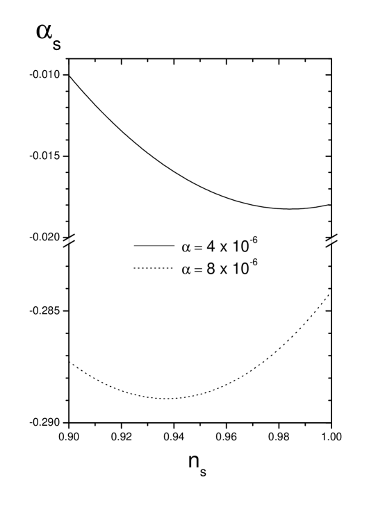
Figure 1: Evolution of the running scalar spectral index $\alpha_{s}$ versus the scalar spectrum index $n_{s}$, for two different values of the parameter $\alpha$.

V Conclusions

In this paper we have studied the tachyon-Chaplygin inflationary model. In the slow-roll approximation we have found a general relation between the tachyonic potential and its derivative. This has led us to a general criterium for inflation to occur (see Eq.(12)). We have also obtained explicit expressions for the corresponding scalar spectrum index $n_{s}$ and its running $\alpha_{s}$.

By using an exponential potential with $\alpha$ fixed (see Eq.(23)) and from the WMAP three year data, we found the values of the parameter $A$ and an upper limit for the tachyon potential $V_{*}$. In order to bring some explicit results we have taken $\alpha=4\times 10^{-6}m_{p}$ and $n_{s}=0.97$, from which we get the values $A\simeq 2\times 10^{-23}m_{p}^{8}$, $V_{*}\simeq 5\times 10^{-13}m_{p}^{4}$ and $\alpha_{s}\simeq-0.02$. The restrictions imposed by currents observational data allowed us to establish a small range for the parameter $\alpha$, which become $10^{-6}<\alpha/m_{p}\lesssim 10^{-5}$. From this range, and from Eqs.(29) and (30), we obtained the ranges $0<A/m_{p}^{8}\lesssim 10^{-23}$ and $8.5\times 10^{-14}\lesssim V_{*}/m_{p}^{4}<8.5\times 10^{-12}$.

In the context of the curvaton scenario, we gave an estimation of the reheating temperature, when the curvaton decay occurs after it dominates. However, a more accurate calculation for the reheating temperature $T_{rh}$ in the curvaton scenario, would be necessary for establishing some constrains on other parameters appearing in our model. We hope to return to this point in the near future.

- (1) A. Guth, Phys. Rev. D 23, 347 (1981).
- (2) A. Albrecht and P. J. Steinhardt, Phys. Rev. Lett. 48, 1220 (1982); A complete description of inflationary scenarios can be found in the book by A. Linde , Particle physics and inflationary cosmology (Gordon and Breach, New York, 1990).
- (3) D. N. Spergel, Astrophys. J. Suppl. 148, 175 (2003); H.V. Peiris, Astrophys. J. Suppl. 148, 213 (2003); D. N. Spergel et al., Astrophys. J. Suppl. 170, 377 (2007).
- (4) A. Sen, JHEP 0204, 048 (2002).
- (5) A. Sen, Mod. Phys. Lett. A 17, 1797 (2002).
- (6) M. Sami , P. Chingangbam and T. Qureshi, Phys. Rev. D 66, 043530 (2002).
- (7) G. W. Gibbons, Phys. Lett. B 537, 1 (2002).
- (8) M. C. Bento, O. Bertolami and A. Sen, Phys. Rev. D 66, 043507 (2002).
- (9) A. Kamenshchik, U. Moschella and V. Pasquier, Phys. Lett. B 511, 265 (2001); N. Bilic, G. B. Tupper and R. D. Viollier, Phys. Lett. B 535, 17 (2002).
- (10) H. B. Benaoum, arXiv:hep-th/0205140; A. Dev, J.S. Alcaniz and D. Jain, Phys. Rev. D 67 023515 (2003); G. M. Kremer, Gen. Rel. Grav. 35, 1459 (2003); R. Bean, O. Dore, Phys. Rev. D 68, 023515 (2003); Z.H. Zhu, Astron. Astrophys. 423, 421 (2004); H. Sandvik, M. Tegmark, M. Zaldarriaga and I. Waga, Phys. Rev. D 69, 123524 (2004) ; L. Amendola, I. Waga and F. Finelli, JCAP 0511, 009 (2005); P.F. Gonzalez-Diaz, Phys. Lett. B 562, 1 (2003) ; L.P. Chimento, Phys. Rev. D 69, 123517 (2004); L.P. Chimento and R. Lazkoz, Phys. Lett. B 615, 146 (2005); U. Debnath, A. Banerjee and S. Chakraborty, Class. Quant. Grav. 21, 5609 (2004); W. Zimdahl and J.C. Fabris, Class. Quant. Grav. 22, 4311 (2005); P. Wu and H. Yu,Class. Quant. Grav. 24, 4661 (2007); M. R. Setare, Phys. Lett. B 654, 1 (2007); M. Bouhmadi-Lopez and R. Lazkoz, Phys. Lett. B 654, 51 (2007).
- (11) M.C. Bento, O. Bertolami and A. Sen, Phys. Lett. B 575, 172 (2003); M.C. Bento, O. Bertolami and A.A. Sen, Phys. Rev. D67, 063003 (2003).
- (12) M. Makler, S.Q. de Oliveira and I. Waga, Phys. Lett. B 555, 1 (2003); J.C. Fabris, S.V.B. Goncalves and P.E. de Souza, arXiv:astro-ph/0207430; M. Biesiada, W. Godlowski and M. Szydlowski, Astrophys. J. 622, 28 (2005); Y. Gong and C.K. Duan, Mon. Not. Roy. Astron. Soc. 352, 847 (2004); Y. Gong, JCAP 0503, 007 (2005) .
- (13) O. Bertolami and V. Duvvuri, Phys. Lett. B 640, 121 (2006).
- (14) G. A. Monerat et al., Phys. Rev. D 76, 024017 (2007).
- (15) T. Barreiro, A.A. Sen, Phys. Rev. D 70, 124013 (2004).
- (16) L. Randall and R. Sundrum, Phys. Rev. Lett. 83, 4690 (1999); T. Shiromizu, K. Maeda and M. Sasaki, Phys. Rev. D 62, 024012 (2000); D. Dvali, G. Gabadadze and M. Porrati, Phys.Lett. B 485, 208 (2000); K. Freese and M. Lewis, Phys. Lett. B 540, 1 (2002); R. Maartens, Lect. Notes Phys. 653 213 (2004); A. Lue, Phys. Rept. 423, 1 (2006).
- (17) M. Fairbairn and M. H. G. Tytgat, Phys. Lett. B 546, 1 (2002).
- (18) J. C. Hwang and H. Noh, Phys. Rev. D 66, 084009 (2002).
- (19) J.M. Bardeen, Phys. Rev. D 22, 1882 (1980); B. A. Bassett, S. Tsujikawa and D. Wands, Rev. Mod. Phys. 78, 537 (2006).
- (20) D. A. Steer and F. Vernizzi, Phys. Rev. D 70, 043527 (2004).
- (21) M. Tegmark et al., Phys. Rev. D 69, 103501 (2004).
- (22) D. Kutasov, M. Marino and G. W. Moore, JHEP 0010, 045 (2000).
- (23) A. de la Macorra, U. Filobello and G. German, Phys. Lett. B 635, 355 (2006)
- (24) G. N. Felder, L. Kofman and A. Starobinsky, JHEP 0209, 026 (2002).
- (25) C. Campuzano, S. del Campo, and R. Herrera, Phys. Rev. D 72, 083515 (2005), [Erratum-ibid. D 72, 109902 (2005)]; C. Campuzano, S. del Campo and R. Herrera, Phys. Lett. B 633, 149 (2006).
- (26) L. F. Abbott, E. Fahri and M. Wise Phys. Lett. B 117, 29 (1982); F. Di Marco, F. Finelli and R. Brandenberger, Phys. Rev. D 67, 063512 (2003).
- (27) B. A. Bassett, S. Tsujikawa and D. Wands, Rev. Mod. Phys. 78, 537 (2006).
- (28) L. Kofman and A. Linde, JHEP 0207, 004 (2002).
- (29) G. Felder, L. Kofman and A. Linde, Phys. Rev. D 60, 103505 (1999).
- (30) B. Feng and M. Li, Phys. Lett. B 564, 169 (2003).
- (31) F. Lucchin and S. Matarrese, Phys. Rev. D 32, 1316 (1985); S. Mollerach, Phys. Rev. D 42, 313 (1990); D. H. Lyth and D. Wands, Phys. Lett. B 524, 5 (2002); G. Efstathiou, Mon. Not. Roy. Astron. Soc. 346, L26 (2003); A. Mazumdar and M. Postma, Phys. Lett. B 573, 5 (2003) [Erratum-ibid. B 585, 295 (2004)].
- (32) C. Campuzano, S. del Campo and R. Herrera, JCAP 0606, 017 (2006); S. del Campo and R. Herrera, Phys. Rev. D 76, 103503 (2007); J. C. Bueno Sanchez and K. Dimopoulos, JCAP 11, 007 (2007).