Nonlinear force-free magnetic field extrapolations: comparison of the Grad-Rubin and Wheatland-Sturrock-Roumeliotis algorithm

Abstract

We compare the performance of two alternative algorithms which aim to construct a force-free magnetic field given suitable boundary conditions. For this comparison, we have implemented both algorithms on the same finite element grid which uses Whitney forms to describe the fields within the grid cells. The additional use of conjugate gradient and multigrid iterations result in quite effective codes.

The Grad-Rubin and Wheatland-Sturrock-Roumeliotis algorithms both perform well for the reconstruction of a known analytic force-free field. For more arbitrary boundary conditions the Wheatland-Sturrock-Roumeliotis approach has some difficulties because it requires overdetermined boundary information which may include inconsistencies. The Grad-Rubin code on the other hand loses convergence for strong current densities. For the example we have investigated, however, the maximum possible current density seems to be not far from the limit beyond which a force free field cannot exist anymore for a given normal magnetic field intensity on the boundary.

1 Introduction

With the advent of vector magnetographs which measure the line-of-sight component of the photospheric magnetic field and, except for a 180^∘ ambiguity, also its component normal to the line-of-sight, the interest in extrapolating these measurements into the corona have grown enormously.

The line-of-sight component of the photospheric magnetic field has been observed for decades now but these measurements alone supply only boundary information at best sufficient for a Laplace field model of the coronal magnetic field. The vector magnetograph observations now available considerably constrain the photospheric horizontal field and allow estimates also of the coronal current density. As a consequence much more realistic coronal field models can be based on these observations.

Since the magnetic field, at least in the lower corona, completely dominates the plasma forces, a “force-free” approximation of the field for stationary situations seems to be a tolerable assumption. “Force” in this context means the magnetic Lorentz force $\vec{j}\!\times\!\vec{B}$. All other MHD forces like gravity, pressure, etc. are neglected because they are about three orders of magnitude smaller than $jB$. Hence, the current and magnetic field vectors should be aligned to better than half a degree.

These simplifications accepted, the magnetic field in some domain $V$ of the corona may be described by

$$\boldsymbol{\nabla}\!\cdot\!\vec{B}=0\;;\quad\boldsymbol{\nabla}\!\times\!\vec{B}=\vec{j}\;;\quad\vec{j}\!\times\!\vec{B}=0\,.$$ (1)

The alignment of current and magnetic field causes the problem to be nonlinear, hence the questions which boundary information is to be supplied and how to solve (1) are by no means trivial.

Boundary conditions which seem necessary and sufficient for (1) are (Boulmezaoud and Amari,, 2000)

$$\vec{n}\!\cdot\!\vec{B}\hskip 5.0pt\mbox{on}\hskip 5.0pt\partial V\;;\quad\vec{n}\!\cdot\!\boldsymbol{\nabla}\!\times\!\vec{B}\hskip 5.0pt\mbox{on}\hskip 5.0pt(\partial V)^{-}\hskip 5.0pt\mbox{or}\hskip 5.0pt(\partial V)^{+}\,,$$ (2)

where $(\partial V)^{\pm}$ is that part of the surface of $V$ where $\vec{n}\!\cdot\!\vec{B}$ is either $>$ 0 or $<$ 0. But not all the boundary values which comply with (2) are allowed. The field line twist which can be stationarily maintained, i.e., $\vec{n}\!\cdot\!\boldsymbol{\nabla}\!\times\!\vec{B}$ on $\partial V$, is limited by the field energy sustained from the exterior, i.e., by $\vec{n}\!\cdot\!\vec{B}$ (see section 5.2).

Quite some effort has gone into attempts to solve (1) for given boundary values either in the form (2) or differently. Among the most promising schemes are those suggested a long time ago by Grad and Rubin (1958, abbreviated GR) and more recently by Wheatland, Sturrock, and Roumeliotis (2000, abbreviated WSR). The GR code has first been implemented by Sakurai (1981) and further developed by Amari et al. (1999), Régnier et al. (2002) and Wheatland (2004). The WSR scheme has been extended by Wiegelmann (2004) and Wiegelmann and Inhester (2003). The development still is an active area of research. A comparison and description of codes in use and other alternative approaches can be found in Schrijver et al. (2006).

A difficulty for a thorough comparison of the various schemes, however, is the fact that they are often implemented very heterogeneously and also include many different details which could easily speed up or slow down their performance and sometimes may even obscure the basic advantages or disadvantages of an approach.

In order the make the two schemes comparable, we apply them to the same problem defined on exactly identical grids. Error norms to measure the performance are exactly the same. The special grid which we use is explained in section 2. We are convinced that it has many advantages for electromagnetic problems like (1).

The WSR and the GR algorithms have been extensively described elsewhere, so that in sections 3 and 4 we restrict ourselves to the basics and rather emphasize some or the details of our implementation. The numerical results obtained for two different examples are presented and discussed in the final parts 5 and 6.

2 The grid

For the problem we want to investigate the choice of the grid and the representation of the fields is very crucial. We found most suitable for our purposes a finite element grid which allows to transform standard vector analysis consistently into discrete space. It is related to finite difference grids with staggered field components and similar grids based on Yee’s scheme (Yee,, 1966). In part of the mathematical literature these special finite elements are called discrete Whitney forms (Bossavit,, 1988) because they have very much in common with continuous differential forms. In fact, some of the finite elements have been known for a long time, however, the way they are related among each other by differentiation operations and to their dual space analogues is relatively new and a matter of current research (Hiptmair,, 2001; Grădinaru,, 2002). The elements are particularly suited for a numerical treatment of electromagnetic fields (Teixeira,, 2001).

We here use the elements in the most simple form to lowest order and on a regular cubic grid which spans our computational domain, a square box $V$ = $[0,1]\times[0,1]\times[0,1]$. The $n$$\times$$n$$\times$$n$ grid cells each have a size $h$ = $1/n$. The cell vertices are located at $ih$, $i=0,n$; the cell centres are at $(i-0.5)h$, $i=1,n$.

Figure 1: Lowest order Whitney forms for a square grid cell.

In Figure 1 we present the four types of finite elements which we use here. Each form a Hilbert space of either scalar or vector valued piecewise first or zero order polynomials determined by a set of parameters which are representative averages of the field to be described. The respective averaging areas are indicated in colour.

Lagrangian elements (0-forms) have as parameters the function values at the 8 vertices of a cell. The element function is linear inside the grid cell such that the correct values are met at the vertices.

The Nédélec elements (1-forms, Nédélec, 1986) are a discrete representation of a vector field. Its element parameters are the averages of a field component over a cell edge along the respective component direction. The element function is constant along the edge and varies linearly in transverse direction matching the right values at the four cell edges of the given direction.

The Raviart-Thomas element (2-forms, Raviart and Thomas, 1977) has as element parameters the face averages of the field component normal to the face. The element function varies linearly in this normal direction and is constant across the face plane.

The last element we need is a finite volume element (3-form) for a scalar function approximation. It has only a single parameter per grid cell which represents the average of the scalar over the entire cell.

Every vector differential operation transforms an $n$-form element in a natural way into a $n\!+\!1$-form element:

As for continuous differential forms, a double differentiation gives exactly a zero field and insures thus that curl$\circ$grad and div$\circ$curl vanish identically also for the discrete forms. This vanishing of double differentiation is not a consequence of the precision with which we approximate the differentiation of discrete forms but is due to the fact that the boundary of a boundary is an empty set, hence is a consequence of geometry alone (Jänich,, 2001). It is therefore not surprising that this rule holds also for discrete forms.

Figure 2: Dual grid cell in relation to a primary (coloured) grid cell.

In order to allow for Laplacians, the alternative combination of vector differential operators, we need to introduce the dual grid as opposed to the primary grid described above. The dual grid is in case of the regular square primary grid again a square grid but shifted by half a grid size in each axis direction such that vertices of the dual grid are located at the cell centres of the primary grid (see Figure 2). Hence there is a natural association between primary 3-forms and dual 0-forms. This association also holds for the other forms, between the $n$-forms of the dual grid and primary $(3-n)$-forms. For general grids this association is manifested by the Hodge (or $\star$) transform (Hiptmair,, 2001). For the square grid we use here, the Hodge transform is simple because the finite element parameters of the dual form are the same as the corresponding parameters of the primary element (except for domain boundary effects). Note, however, that while the finite element parameters remain unaltered under this transformation, their interpretation and their functional representation changes.

Of course, the forms of the dual grid are connected among each other by differentiations in the same way as for the primary grid. The final pattern of forms together with the mappings among them yields

In this scheme, the usual 6-point stencil of a discrete Laplacian operated on a 0-form can be realized by div$\star$grad where the star denotes the Hodge transform and the result is a dual 3-form. Likewise, the Laplacian on a 1-form can be written as div$\star$grad $-$ curl$\star$curl and returns a dual 2-form. Except for boundary effects, the primary and dual grids are on equal footing.

For our problem, the magnetic field $\vec{B}$ is considered a primary 1-form (or dual 2-form). The current density $\vec{j}$ then is a primary 2-form. With these prescriptions, we can perform all differential operation on scalar and on vector fields in a consistent way.

We just mention in passing that these forms can be equally well constructed on an irregular grid and element functions can be higher order polynomials if more element parameters are adequately provided. Hence high order difference formulas can be set up in a systematic way. Multigrid extensions of the Whitney forms are a matter of current research (Grădinaru,, 2002).

3 The Wheatland-Sturrock-Roumeliotis (WSR) algorithm

The algorithm proposed by Wheatland, Sturrock, and Roumeliotis (2000) tries to find the force-free field $\vec{B}$ from the argument which minimizes a penalty function $L$, i.e.,

$$\vec{B}=\mathrm{argmin}(L)\;,\quad L(\vec{B})=\int\limits_{V}|w\vec{j}\!\times\!\vec{B}|^{2}+\int\limits_{V}|\boldsymbol{\nabla}\!\cdot\!\vec{B}|^{2}\,.$$ (3)

In fact, the integrals can be looked upon as a Hilbert product on the respective finite element space defined in the previous section. This conception helps greatly when programming $L$ and its derivatives. The calculation of $\boldsymbol{\nabla}\!\cdot\!\vec{B}$ and $\boldsymbol{\nabla}\!\times\!\vec{B}$ throughout $V$ requires the knowledge of $\vec{n}\!\cdot\!\vec{B}$ and $\vec{n}\!\times\!\vec{B}$ on the whole of the surface $\partial V$. This is more than (2) prescribes and the problem of minimising $L$ under these restrictive conditions is clearly overdetermined. If inconsistent boundary conditions are imposed on (3), a decent minimum may never be reached. We therefore allow for the option in our program to vary the normal and/or tangential field components on individual faces of $V$. This essentially is equivalent to setting $\vec{n}\!\cdot\!\vec{B}$ from $\boldsymbol{\nabla}\!\cdot\!\vec{B}$ = 0 and $\vec{n}\!\times\!\vec{B}$ consistent with a vanishing Lorentz force on the respective boundary face.

In this sense the second integral in (3) is calculated from the squared (dual) 3-form $\boldsymbol{\nabla}\!\cdot\!\vec{B}$ defined at the cell vertices by summing over all vertices. Vertices on a domain surface, edge or corner are especially weighted with factor 0.5, 0.25 and 0.125 respectively.

Figure 3: Finite element parameters entering into the calculation of the $z$ component of $\vec{j}\!\times\!\vec{B}$ at the cell centre. The red arrows on the cell edges denote magnetic field components, the blue face centered arrows the current components involved.

The $\vec{j}\!\times\!\vec{B}$ integral is a little more involved. Formally the exterior product of a 1-form and a 2-form should give a 3-form. Hence the $\times$ product here has not the property of an exterior product in differential geometry. Yet a 3-form, however one for each component of $\vec{j}\!\times\!\vec{B}$ individually, gives the most compact stencil for this expression. In Figure 3 we show the element parameters which are needed for the $z$ component of the Lorentz force at a cell centre. E.g., the contribution $j_{x}B_{y}$ is obtained from an average over the two $x$-faces of the cell. For each of these faces, $j_{x}B_{y}$ is calculated by multiplying $j_{x}$ at its centre with the average of the two $B_{y}$ values from the two $y$-edges of this face. The integral in (3) then is a simple sum over all three components of the Lorentz force. For each component, the respective squared 3-form elements are summed over all cell centres.

In order to obtain argmin $L(\vec{B})$, WSR proposed a simple Landweber scheme by iteratively advancing

$$\vec{B}^{(i+1)}=\vec{B}^{(i)}+s\,\delta\vec{B}^{(i)}\;,\quad\delta\vec{B}^{(i)}=-\frac{\partial L}{\partial\vec{B}}(\vec{B}^{(i)})\,,$$ (4)

which guarantees that $L$ decreases at every step provided step size $s$ is small enough. In this scheme, improvements of $\vec{B}$ are strictly along the negative gradient direction and step sizes are only guessed and reduced if necessary.

We have instead implemented an unpreconditioned conjugate gradient iteration which at every iteration step performs an exact line search to the minimum of $L^{\prime}(s)$ = $L(\vec{B}+s\,\delta\vec{B})$ along the respective search direction. Moreover, it selects an improved search direction $\delta\vec{B}$ instead of the gradient as in (4).

Note that in contrast to existing implementations of this scheme by Wheatland, Sturrock, and Roumeliotis, (2000) or Wiegelmann (2004) who programmed the discretization of the analytical derivative (4), we always calculate the numerically more consistent derivative of the discretized function $L$.

Conjugate gradient solvers are optimal for linear problems for which the objective function $L$ depends to second order on the components of $\vec{B}$. Our problem, however, is nonlinear and (3) is of fourth order in $\vec{B}$ through the $\vec{j}\!\times\!\vec{B}$ term. We make use of our formulation of (3) on the special grid introduced in the previous section in order to calculate all five polynomial coefficients of $L^{\prime}(s)$ in one go. This enables us to perform the exact line search at every step without much effort by a single function call. From the new minimum, the new search direction $\delta\vec{B}^{(i+1)}$ is chosen so that it is a descent direction and also $H$-orthogonal to the previous search direction $\delta\vec{B}^{(i)}$. $H$ here is the local Hessian $\partial^{2}L/\partial B_{i}\partial B_{j}$ at the line search minimum. Likewise, we can also choose the Hestenes-Stiefel variant which yields a new search direction which is $H$-orthogonal with respect to some average Hessian $H$.

A parameter still to be determined in (3) is $w$. Its choice will be discussed later along with the presentation of the results. In fact, it will turn out to be favourable to make it a space-dependent $w(\vec{x})$. This is another difference with respect to the implementations of Wheatland, Sturrock, and Roumeliotis, (2000) and Wiegelmann(2004), who took $w$ a function of $\vec{B}$.

4 The Grad-Rubin (GR) algorithm

Several variations of this algorithm exist. While the previous approach to find a force-free field reduced the problem to a formal optimization procedure, the approach by Grad and Rubin (1958) is inspired by a quasi-physical relaxation: at any time in the iteration the current $\vec{j}$ = $\alpha^{(n)}\vec{B}^{(n)}$ produces via the Biot-Savart law a new field $\vec{B}^{(n+1)}$. According to the differences between $\vec{B}^{(n+1)}$ and $\vec{B}^{(n)}$, $\alpha$ is then redistributed along the new field lines giving rise to a new current and hence a new Biot-Savart field.

In our code, we distribute $\alpha$ along given field lines by solving

$$\vec{B}^{(n)}\!\cdot\!\boldsymbol{\nabla}\alpha^{(n)}=0$$ (5)

for given $\vec{B}^{(n)}$ and boundary values for $\alpha$ on $\partial V$. In the next step we correct the field by solving for the vector potential $\delta\vec{A}$ of the field update

$$\Delta\,\delta\vec{A}=\delta\vec{j}\,,$$ (6)

$$\hskip 5.0pt\mbox{where}\hskip 5.0pt\boldsymbol{\nabla}\!\cdot\!\,\delta\vec{A}=0\hskip 5.0pt\mbox{and}\hskip 5.0pt\delta\vec{j}=\boldsymbol{\nabla}\!\times\!\vec{B}^{(n)}-\alpha^{(n)}\vec{B}^{(n)}\,,$$

with boundary conditions $\vec{n}\!\times\!\,\delta\vec{A}$ = 0 and $(\vec{n}\cdot\boldsymbol{\nabla})\,(\vec{n}\!\cdot\!\delta\vec{A})$ = 0. These boundary conditions insure that $\boldsymbol{\nabla}\!\cdot\!\,\delta\vec{A}$ vanishes also on the domain boundaries. In the subsequent field correction

$$\vec{B}^{(n+1)}=\vec{B}^{(n)}+\boldsymbol{\nabla}\!\times\!\,\delta\vec{A}\,,$$ (7)

the normal components of $\vec{B}$ on the domain boundaries remain unchanged.

In terms of the forms introduced above, the scheme looks as follows:

The scheme basically starts form a potential solution on the left and then cycles the square at the centre. Any time $\vec{B}$ has been updated, $\alpha$ is remapped using (5) before the residual current $\delta\vec{j}$ is calculated. Due to numerical discretization errors in the integration of $\alpha$ in (5), $\delta\vec{j}$ may have a spurious divergence which is checked and if necessary, eliminated by iterating $\boldsymbol{\nabla}\!\cdot\!\delta\vec{j}$ = 0 a few times while preserving normal boundary conditions and $\boldsymbol{\nabla}\!\times\!\delta\vec{j}$.

While the Poisson equation (6) can efficiently be solved with a multigrid solver, the major computational effort is spent in solving (5) to the required precision. Since (5) is first order, boundary values need only be supplied at one end of the field line (or characteristic). With (2) this is automatically satisfied, however this choice of boundary conditions deprives us of the freedom to emphasize those boundary areas where we assume the observations to be more reliable. We therefore do not make the distinction between $(\partial V)^{+}$ and $(\partial V)^{-}$ as in (2) but we safeguard our solver of (5) against inconsistent boundary values for $\alpha$ by attaching a weight with every boundary value for $\alpha$. The final value on the characteristic is the according weighted average from both end points. This way, the influence from uncertain boundary values on the side walls or from imprecise measurements on the bottom (photospheric) boundary can be suppressed.

In principle, (5) is solved by mapping every cell centre along a field line to the boundary and interpolating the boundary values to its foot point. To minimise the number of field line calculations, we store the $\alpha$ value also in every cell the calculated field line intersects along with the intersection coordinates. For about 2/3 of the cells, the field line calculation from their centre then can be discarded, because they have previously been intersected by so many field lines, that their $\alpha$ value can reliably be interpolated form the intersection information stored.

5 Results

We have tested our codes with two different model fields. The first is the Low and Lou (1990) field model, one of the few analytic force free field solutions which now has almost become a standard for tests of force-free reconstruction schemes. For the second test model, a twisted flux tube, we do not have an analytic solution. For the existence of a solution we rely on the symmetry of the boundary conditions supplied.

5.1 Low and Lou model

As a test case model we use the analytical nonlinear force-free field solution of Low and Lou (1990). The field results form a multipole with eigenvalue $a^{2}$ = 0.42659. We placed it at a depth of $l$ = 0.2 below the centre of the ground plane and with orientation in the $x$-$z$ plane with 45 degrees inclination to the $x$ and $z$ axes. The field was scaled so that at the ground plane the vertical field strength ranges between -9.95 and 5.09, the alpha values between -16.9 and 5.61 and the vertical current density between -67.9 and 106. A field line plot of this model is shown in the upper left of Figure 4.

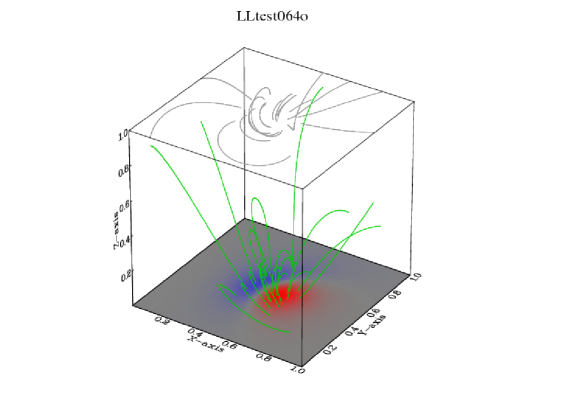
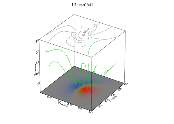
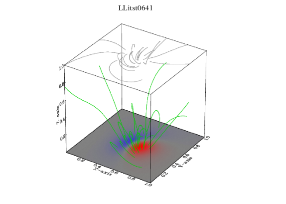
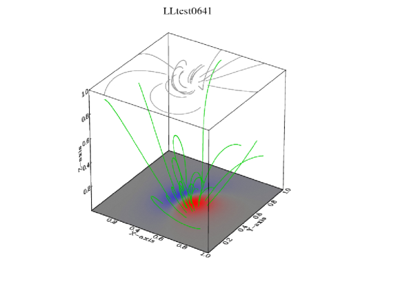
Figure 4: Representative field lines of the original Low and Lou (1990) model (upper left), the result of the WSR iteration with $w$ = const(upper right), the result of the WSR iteration with $w$ = $1/|B_{\mathrm{pot}}|$ (lower left), the result of the GR iteration (lower right). The colour code at the bottom represents $B_{z}$, the top plane shows the vertical projection of the field lines.

The result of the extrapolation is displayed in the other three panels, all for a grid size $n$ = 64. We find that the WSR iteration is strongly biased towards regions where the field strength is large. This very probably is due to the Lorentz force term in (3) which increases with ${\cal O}(B^{4})$. For this reason, the original object function $L$ proposed by WSR (Wheatland, Sturrock, and Roumeliotis,, 2000) had $w$ $\sim$ $1/|\vec{B}|$. This choice, however, makes $L$ a rational function of the $B$ components which we expect to slow down the convergence of the minimization iteration. We therefore prefer the choice $w$ $\sim$ $1/|\vec{B}_{\mathrm{pot}}|$ where $\vec{B}_{\mathrm{pot}}$ is the potential field consistent with the normal component of the given boundary magnetic field. The potential field is obtained easily and our choice of $w$ similarly reduces the influence of regions where the field is expected to be strong. Since $w$ is not changed during the iteration, it does not destroy the analytic properties of $L(\vec{B})$.

The effect of this weighting is remarkable, since $B_{\mathrm{pot}}$ varies by three orders of magnitude between 0.027 and 28 throughout $V$. In Figure 4 we show the result of the WSR iteration with $w$ = const (upper right) and $w$ = const$/|\vec{B}_{\mathrm{pot}}|$ (lower left). The discrepancy of the former at larger heights in regions of small magnetic field strength is immediately apparent. The lower right panel shows the result of the GR iteration. It reproduces the original in weak and strong field regions equally well to at least the plotting precision. Details in the original field lines are reproduced exactly.

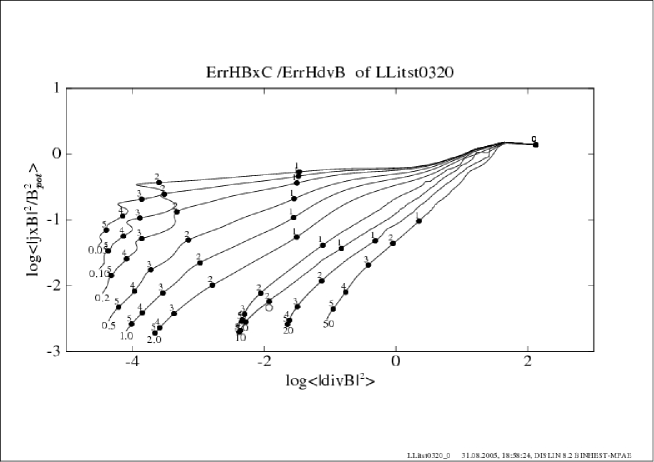
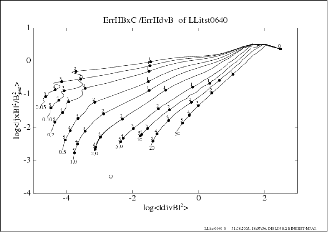
Figure 5: Decrease of the two integral terms in (3) during the conjugate gradient iteration for a grid $n$ = 32 (top) and $n$ = 64 (bottom). The weight function was chosen $w$ = const/$|\vec{B}_{\mathrm{pot}}|$ with different values for the constant as marked at the lower left end of the curves. The tick marks along the curve indicate every 50${th}$ ($n$=32) or 100${th}$ ($n$=64) iteration step. The circle in each diagram indicates the integral values of the analytic model calculated on the respective grid.

For the WSR iteration the question remains how to choose the constant in the weighting factor $w$. In Figure 5 we display the iteration history of the two integral terms in (3) for different constants in $w$ = const$/|\vec{B}_{\mathrm{pot}}|$ and for two different grid sizes $n$ = 32 and 64. The iterations were started with an initial $\vec{B}^{(0)}$ = 0 inside $V$ and the right boundary conditions for the normal and tangential fields on $\partial V$. Note that for $\vec{B}^{(0)}$ the divergence and the Lorentz force do not vanish because of these boundary values imposed.

A value const $\sim$ 1 seems optimal which is not surprising because with this choice of $w$ both terms are of the same order $B^{2}/h$. Smaller values of the constant lead to a faster reduction of the div$\vec{B}$ term, larger values yield a bias towards the elimination of the Lorentz force. In Figure 5 we have chosen the axes scales for the ordinate and the abscissa equally, so that the curve (const $\sim$ 20) which decreases closest to 45 degrees eliminates both integral terms at about equal rates.

For the case $w$ = const similar plots can be produced as in Figure 5 and the optimal constant then is around 0.05. It depends, however, on the magnetic field strength of the model since now the two terms in (3) have different units.

The number of iterations performed in Figure 5 was 10$\times n$ where $n$ is the number of cells along each coordinate axis. From the similarity of both diagrams we conclude that roughly the number of iterations needed to reduce $L$ by a given factor increases proportional to $n$. This result seems to differ from previous implementations of the WSR algorithm which used a Landweber iteration with a more or less effective step size control (Schrijver et al.,, 2006). For these codes, the number of iterations was found to increase with $n^{2}$. Note, however, that these authors measured the number of steps until the magnitude of $\delta\vec{B}$ fell below a given limit rather than the convergence speed (i.e., the fractional decrease of $L$ per iteration step).

Of course, the precision of the analytic model, calculated on the respective grid positions increases with higher grid resolution (see circles in the diagrams in Figure 5). For the $n$ = 32 grid this precision is reached already after 100 iterations with const = 10, while for $n$ = 64 the much higher analytical precision seems to be out of reach.

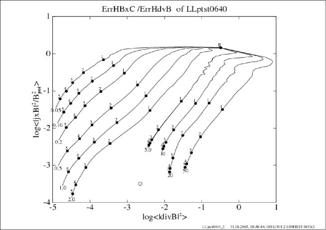
Figure 6: Same as lower diagram in Figure 5, but with a potential field as initial $\vec{B}$ for the iteration.

It is well known that it depends among other details also on the initial iterate $\vec{B}^{(0)}$ how closely a desired solution can be approached by Krylov-type iteration schemes (e.g., Landweber, steepest descent or conjugate gradients). During the iteration, the search directions $\delta\vec{B}^{(i)}$ build up a subspace of the Hilbert space for $\vec{B}$ and discrepancies between the iterate $\vec{B}^{(i)}$ and the solution can at best be eliminated inside this subspace, usually called Krylov space (Saad,, 2003). Differences between $\vec{B}^{(0)}$ and the solution which fall out of the Krylov space cannot be corrected. A good choice of the initial $\vec{B}^{(0)}$ therefore does not only save computation time but may be a necessity to reach a solution at all, at least for ill-posed problems for which the Krylov space remains limited. In Figure 6 we show a diagram similar to the $n$ = 64 case in Figure 5, but here the initial $\vec{B}^{(0)}$ was chosen to be the potential field inside $V$ for the given normal component boundaries but with the tangential field components on $\partial V$ expected for the final force-free field. Note that again the Lorentz force and the divergence of the initial $\vec{B}^{(0)}$ do not vanish because the final, non-potential tangential field boundary values on $\partial V$ have been enforced.

The diagram shows that with this improved initial field, it is no problem to reach the error bounds of the analytical model if const $<$ 5. Note, however, a larger value for the constant, i.e., a greater bias towards the Lorentz force in (3) during the iteration does not necessarily produce a smaller final error of the Lorentz force term.

For the GR scheme, the iterates $\vec{B}^{(i)}$ are always numerically divergence free and at any step they satisfy the normal boundary conditions. We therefore cannot start this iteration from $\vec{B}^{(0)}$ = 0 but take the potential field as a starting point instead. Since the information about the tangential boundary field is stored in the boundary values of $\alpha$, the divergence of $\vec{B}^{(0)}$ and the current $\vec{j}^{(0)}$ exactly vanish in contrast to the WSR initial field.

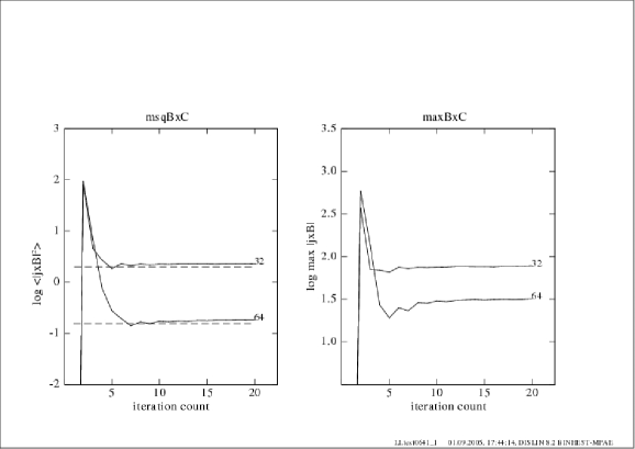
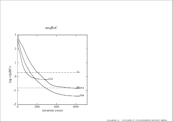
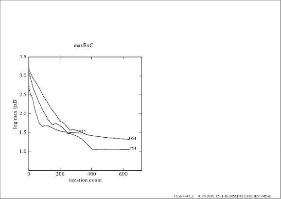
Figure 7: Mean square Lorentz force $<\!|\vec{j}^{(i)}\!\times\!\vec{B}^{(i)}|^{2}\!>$ in the course of the GR (left) and the WSR (right) iteration. For the WSR iteration the constant was chosen to be 2. The curves are the result for the $n$ = 32 and 64 grid as marked. For the latter we show results for an initial $\vec{B}^{(0)}$ = 0 (064) and $\vec{B}^{(0)}$ = $\vec{B}_{\mathrm{pot}}$ (P64) except for the boundary values. The dashed lines denote the respective residual Lorentz force for the discretized Low and Lou (1990) solution $\vec{B}_{\mathrm{org}}$.

Figure 8: Same as Figure 8, but the maximum Lorentz force max$|\vec{j}^{(i)}\!\times\!\vec{B}^{(i)}|$ in $V$ for the GR iteration (left) and the WSR scheme (right).

The GR scheme converges much more rapidly than the WSR algorithm. However, the GR iteration scheme does not guarantee a continuous decrease of a certain object function, such as $L$ for the WSR case. Less than 10 iterations were needed to eliminate the residual Lorentz forces to the level of the discrete Low and Lou solution (see Figure 8 and 8). However, once this level has been reached, the Lorentz forces could not be lowered any further but even increased slightly again. This holds both for the mean and the maximum residual Lorentz force. Note that in Figs. 8 we show the mean square Lorentz force without weight $w$ $\sim$ $1/|B_{\mathrm{pot}}|$ as in Figure6.

From our calculations we may conclude therefore that with a WSR code and a potential field as initial iterate smaller residual Lorentz forces may eventually be reached than with the GR approach, provided the WSR code is supplied with consistent and exact boundary conditions of, e.g., a known analytic force free field. In this case a minimum $L$ = 0 exists and we are confident that our code will approach towards it due to its exact line search capabilities. The number of iterations though may be prohibitive in some cases.

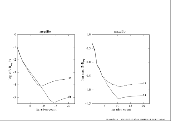
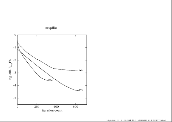
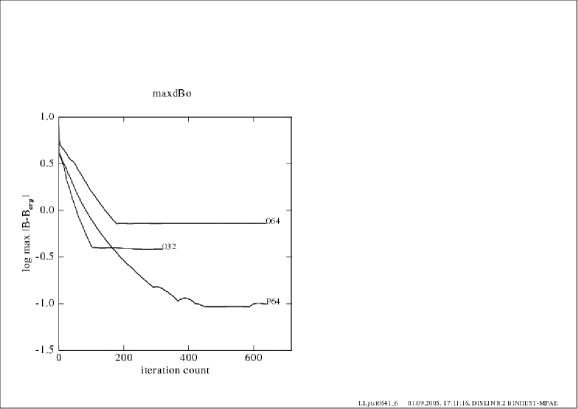
Figure 9: Mean square difference $<\!(\vec{B}^{(i)}-\vec{B}_{\mathrm{org}})^{2}\!>$ of the iterated field to the original Low and Lou (1990) solution for the GR iteration (left) and the WSR scheme (right). The coding of the curves refer to the same calculations as in Figures 8 and 8.

Figure 10: Same as Figure 10, but the maximum difference max$|\vec{B}^{(i)}-\vec{B}_{\mathrm{org}}|$ of the iterated field to the original Low and Lou (1990) solution for the GR iteration (left) and the WSR scheme (right).

We have seen in the field line plots, that the GR result, even though it retains residual Lorentz forces, approaches the discrete Low and Lou solution extremely well. This can be confirmed if the difference $\vec{B}^{(i)}-\vec{B}_{\mathrm{org}}$ is monitored during the iteration. As is shown in Figs. 10 and 10 the GR code here performs much better than WSR. The mean square error it achieves is almost an order of magnitude smaller than the WSR code can reach, even with the potential initial field. It seems that the most consistent field with the least Lorentz forces is reached after only 5 ($n$ = 32) or $\sim$ 7 ($n$ = 64) iterations. Continuation of the iteration brings the field still closer to the Low and Lou solution but increases the level of the Lorentz force slightly. After about 10-14 iterations the difference $\vec{B}^{(i)}-\vec{B}_{\mathrm{org}}$ is minimized and rises thereafter. A critical point for a practical application of the GR code is therefore when to stop the iteration. The saturation of the residual Lorentz forces seems to be a helpful indication.

To measure differences of our final iterate with the original Low and Lou field, we calculate the following two error norms:

$$E_{D}=\frac{\sum\limits_{\mathrm{elements}}\;\sum\limits_{i\in\{x,y,z\}}|B_{i}-(\vec{B}_{\mathrm{org}})_{i}|}{\sum\limits_{\mathrm{elements}}\;\sum\limits_{i\in\{x,y,z\}}|(\vec{B}_{\mathrm{org}})_{i}|}\,,$$

$$E_{C}=\frac{\sum\limits_{\mathrm{elements}}\;\sum\limits_{i\in\{x,y,z\}}|B_{i}\!\cdot\!(\vec{B}_{\mathrm{org}})_{i}|}{\sum\limits_{\mathrm{elements}}\;\sum\limits_{i\in\{x,y,z\}}(\vec{B}_{\mathrm{org}})_{i}^{2}}\,.$$

$E_{D}$ measures a normalized difference to the original field, $E_{C}$ a correlation with it. The two error measures are not independent: for small errors, $1-E_{C}$ $\sim$ $E_{D}^{2}$. Note that we do not subtract or correlate vectors but every individual component because from our grid, we obtain the values for different components at different locations. For the final GR result on a $n$ = 64 grid, we obtain

$$E_{D}=3.81\;10^{-3}\;;\quad E_{C}=1.000034$$

after 14 iteration steps which took 18 minutes of calculation on a 667 MHz Pentium IV Linux operated single processor with 256 MB Ram. The residual Lorentz forces of the reconstructed field had the same level as the discretized original Low and Lou field and the divergence was of the order of the numerical roundoff error.

The equivalent WSR computations starting from $\vec{B}^{(0)}$ = $\vec{B}_{\mathrm{pot}}$ yield

$$E_{D}=1.81\;10^{-2}\;;\quad E_{C}=0.99947$$

after 640 iteration steps and 22 minutes of calculation time on the same computer. The mean square residual Lorentz forces of the reconstructed field could be reduced to about a third of those of the discretized original Low and Lou field, its divergence to 1/80 of $<\!(\boldsymbol{\nabla}\!\cdot\!\vec{B}_{\mathrm{org}})^{2}\!>$.

5.2 Twisted loop

As a second experiment we tried to model a twisted magnetic loop with the $\alpha$ amplitude as a free parameter. The boundary conditions for the GR iterations were chosen in the following way:

$$\vec{n}\!\cdot\!\vec{B}=0\hskip 5.0pt\mbox{and}\hskip 5.0pt\alpha=0\hskip 5.0pt\mbox{on}\hskip 5.0pt\partial V/\{\vec{x}\,|\,z=0\}\,,$$

$$\hat{\vec{z}}\!\cdot\!\vec{B}=\sum_{\sigma=\pm}\sigma\exp-\frac{(\vec{x}-\vec{x}_{\sigma})^{2}}{r^{2}}\hskip 5.0pt\mbox{and}\hskip 5.0pt\alpha=\alpha_{\mathrm{max}}|\hat{\vec{z}}\!\cdot\!\vec{B}|\hskip 5.0pt\mbox{on}\hskip 5.0pt\partial V\!\cap\!\{\vec{x}\,|\,z=0\}\,,$$ (8)

where $\vec{x}_{\sigma}$ = $(0.5-0.2\sigma,0,0)^{T}$ and $r$ = 0.1. Since $|\hat{\vec{z}}\!\cdot\!\vec{B}|$ has a maximum of 1, $\alpha_{\mathrm{max}}$ measures the maximum magnitude of $\alpha$ of our boundary values. We also rely on the symmetry of the boundary conditions and do not make the distinction between $(\partial V)^{\pm}$ as is formally necessary (see eq. 2). Rather, we would like to see our weighting mechanism (see section 4) at work. All weights were set to unity. The grid size was chosen as $n$ = 64.

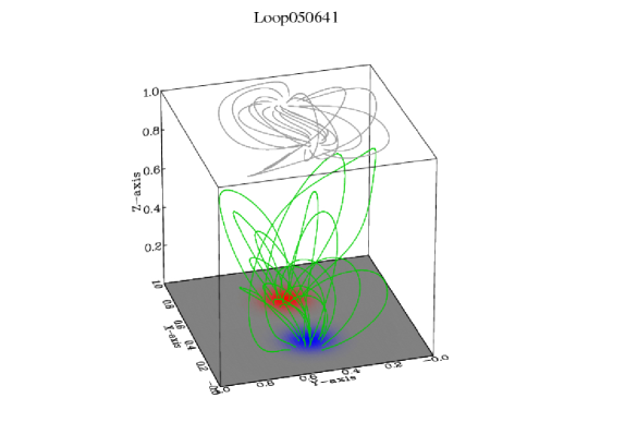
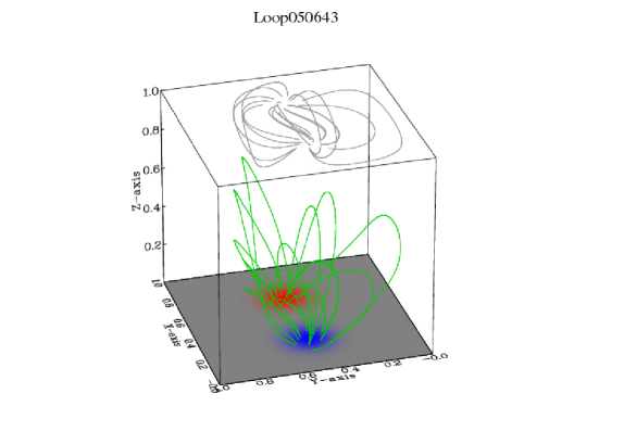
Figure 11: Representative field lines of the reconstructions of the twisted loop model by the GR (left) and WSR (right) algorithms. In both cases $\alpha_{\mathrm{max}}$ = 5 was chosen. The colour code at the bottom represents $B_{z}$, the top plane shows the vertical projection of the field lines. The starting points of the field lines were chosen identically for both model results.

For the equivalent WSR calculations, we need to transform (8) into the full field vector on the domain boundary. However only the in-plane curl, $\vec{n}\!\times\!\boldsymbol{\nabla}\!\times\!\vec{B}$ on $\partial V$ is determined by the $\alpha$ boundary values. We therefore use the boundary fields from the GR results as boundary conditions for the WSR calculations. The local maximum discrepancy between $\alpha$ as prescribed in (8) and the GR result was less than 10%.

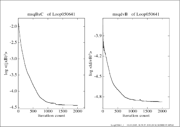
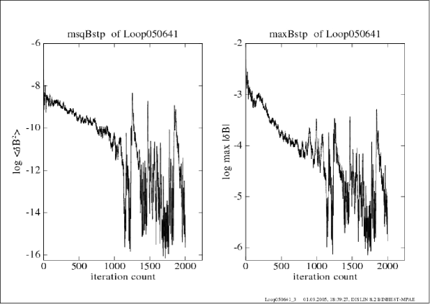
Figure 12: Mean square Lorentz force (left) and magnetic field correction step $\delta\vec{B}$ (right) for the twisted loop model reconstruction by the WSR code. The boundary conditions chosen correspond to $\alpha_{\mathrm{max}}$ = 5.

In Figure 11 we present the results of the different algorithms for a value $\alpha_{\mathrm{max}}$ = 5. A visual inspection reveals that the low lying loops correspond well in shape, however the outer loops from the GR reconstruction show much more twist than those produced with the WSR code. The reasons for this difference may be twofold: The WSR result has the larger residual Lorentz forces (see Figure 12) and it took almost 2000 iterations until a level was reached from which $<\!(\vec{j}\!\times\!\vec{B})^{2}\!>$ could not be lowered any further. In the course of this WSR iteration we observed that the twist of the outer field lines developed only very late. A continuation of the iteration may therefore bring a slight improvement towards the shape of the GR produced field lines.

The GR iterations, on the other hand, probably overtwist the outer loops. The reason is the integration of $\alpha$ along field lines in (5). On the ground surface the vertical current density $\alpha B_{z}$ is confined to only two small concentrated spots $\sim$ $\exp-2(\delta\vec{x}/r)^{2}$ of less than 10 grid spacings in diameter. Even though we take great care to follow as closely as possible the characteristics when we solve (5), a slight diffusion of $\alpha$ off the characteristics can probably not be avoided. The diffused current density probably causes a stronger twist for the outer field lines than is realistic.

The twisted loop model was designed to see how the codes behave when $\alpha$ is enhanced. We pursued this question only for the GR code. The amount of twist with which a field line can be charged, i.e., the magnitude of $\alpha_{\mathrm{max}}$ is limited by the virial theorem (Molodensky,, 1969). The virial theorem states that for a sphere of radius $R$

$$\int\limits_{V}|\vec{B}|^{2}=R\int\limits_{\partial V}\big{(}|\vec{n}\!\cdot\!\vec{B}|^{2}-|\vec{n}\!\times\!\vec{B}|^{2}\big{)}\,.$$ (9)

For a half space (i.e., $R$ $\rightarrow$ $\infty$) this reduces to

$$\int\limits_{z=0}\big{(}|\hat{\vec{z}}\!\cdot\!\vec{B}|^{2}-|\hat{\vec{z}}\!\times\!\vec{B}|^{2}\big{)}\;\downarrow\;0\,.$$ (10)

This is in fact one of the relations enforced by the preprocessing scheme for the boundary data by Wiegelmann et al. (2005). We can express the surface field in terms of a potential and a stream function

$$\hat{\vec{z}}\!\times\!\vec{B}=\hat{\vec{z}}\!\times\!\boldsymbol{\nabla}\phi-\boldsymbol{\nabla}\psi\,,$$

and it is clear that both $\phi$ and $\psi$ will depend on the shape and amplitude of the $\alpha$ boundary condition at $z$ = 0. If the boundary conditions are chosen as in (8), then

$$\Delta\psi(\alpha)=\hat{\vec{z}}\!\cdot\!\vec{j}=\alpha(\hat{\vec{z}}\!\cdot\!\vec{B})=\alpha_{\mathrm{max}}|\hat{\vec{z}}\!\cdot\!\vec{B}|(\hat{\vec{z}}\!\cdot\!\vec{B})\,.$$

The last step is due to the rigid connection between $\alpha$ and $B_{z}$ in (8). Hence the stream function $\psi$ is directly proportional to $\alpha_{\mathrm{max}}$ and invariable in its shape. To keep the balance in (10), $|\boldsymbol{\nabla}\phi(\alpha_{\mathrm{max}})|$ has to decrease as $|\boldsymbol{\nabla}\psi(\alpha_{\mathrm{max}})|$ grows with $\alpha_{\mathrm{max}}$. Setting $\psi(\alpha_{\mathrm{max}})$ = $\alpha_{\mathrm{max}}\psi(1)$ and making use of the orthogonality (due to the symmetry in (8) about $x$ = 0.5) of the two fields $\hat{\vec{z}}\!\times\!\boldsymbol{\nabla}\phi$ and $\boldsymbol{\nabla}\psi$ on the plane $z$ = 0 we obtain from (10):

$$\alpha_{\mathrm{max}}^{2}\leq\frac{\int\limits_{z=0}\big{(}|B_{z}|^{2}-|\boldsymbol{\nabla}\phi(\alpha_{\mathrm{max}})|^{2}\big{)}}{\int\limits_{z=0}|\boldsymbol{\nabla}\psi(1)|^{2}}\leq\frac{\int\limits_{z=0}|B_{z}|^{2}}{\int\limits_{z=0}|\boldsymbol{\nabla}\psi(1)|^{2}}\,.$$

A definite upper bound for $|\alpha_{\mathrm{max}}|$ is therefore reached when $|\boldsymbol{\nabla}\phi(\alpha_{\mathrm{max}})|$ has declined to 0. Numerically, we obtain for (8): $\int_{z=0}|B_{z}|^{2}$ = 0.031 and $\int_{z=0}|\boldsymbol{\nabla}\psi(1)|^{2}$ = 0.00011 which gives $|\alpha_{\mathrm{max}}|$ $\lesssim$ 16 as upper bound. Since $|\boldsymbol{\nabla}\phi(\alpha_{\mathrm{max}})|^{2}$ probably never becomes zero, a realistic upper bound is much less than this crude estimate.

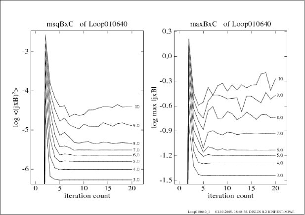
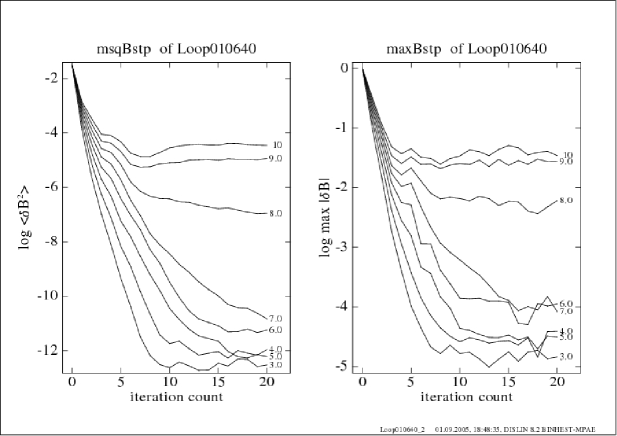
Figure 13: Mean square Lorentz force (left) and magnetic field correction step $\delta\vec{B}$ (right) for the twisted loop model with different amplitudes $\alpha_{\mathrm{max}}$ in the course of the GR iteration. The respective values of $\alpha_{\mathrm{max}}$ are attached to the curve. Note the different ordinate scales compared to Figure 12.

In the GR iterations of the twisted loop model we varied $|\alpha_{\mathrm{max}}|$ in the range [0,10]. We observe that the convergence drastically decreases and comes to a halt between $|\alpha_{\mathrm{max}}|$ = 7 and 8 (see Figure 13). We presume that this loss of convergence is not a failure of the code but it rather indicates the upper limit of feasible values of $|\alpha_{\mathrm{max}}|$. Beyond this limit, a stationary force-free solution with a boundary as in (8) probably is not possible. Note that this transition is not so well visible in the residual Lorentz forces which continually rise as $|\alpha_{\mathrm{max}}|$ and hence the general level of the current density increases.

A point worthy of investigation is how the above estimate of the maximum current density of a stationary force free flux tube complies with the kink instability threshold for twisted flux tubes (e.g., Mikić, Schnack, and van Hoven,, 1990; Van Hoven, Mok, and Mikić, ). This instability criterium predicts stationarity only if the number of turns a field makes around the flux tube axis is less than about 2.4.

6 Discussion

Force-free extrapolation codes available nowadays are capable to compute a field model in boxes as big as 256$\times$256$\times$256 (e.g., Schrijver et al.,, 2006). Compared to the resolution of modern vector magnetograms with pixel arrays of 1000$\times$1000, the calculated extrapolation models are most often quite limited in their resolution. Keeping in mind that they have to oversample the observation in order to limit the discretization error, the observed data typically has to be smoothed before it can serve as boundary condition for an extrapolation (Wiegelmann, Inhester, and Sakurai,, 2005). There is therefore a definite need for fast and effective force-free reconstruction codes which can handle bigger models in order to make proper use of the resolution which the observations provide.

In this paper we have implemented and tested two alternative schemes for the extrapolation of a force-free field from boundary data. The algorithms differ considerably and in order to compare these different approaches unobscured by differences in the numerical coding, we implemented them as far as possible in a similar way. The discretization on a finite element grid by means of Whitney forms results in codes with a very efficient performance. In addition, we have improved the WSR code considerably using an efficient conjugate gradient iteration.

The two schemes differ not only in their approach towards a solution, but they also differ in the boundary information which has to be supplied. The WSR code requires boundary information which clearly overdetermines the problem unless parts of the boundary fields are left to be varied. But the full magnetic field vector on even part of the boundary is a very strong constraint and there is a great danger to impose inconsistent boundary values. This may be one reason why the WSR code converges well for known solutions like the Low and Lou model (Low and Lou,, 1990) where precise and consistent boundary values are supplied, while a little less reliable boundary values like those we retrieved from the result of a GR extrapolation slow down the WSR convergence speed markedly.

The WSR code has as a free parameter the weight between the Lorentz force and the divergence term in (3). In our implementation it is hidden in the constant of the weight function $w$. We found const $\sim$ 1 a good value for the problems which we have delt with here. However, since the (1) is nonlinear, the performance and also the optimal parameters may vary with the problem studied. As an example, note the difference in the iteration history for the Low and Lou model for const = 2 and 5 in Figure 6. Here, the convergence changes drastically if the constant is modified by only a small amount.

Typical computation times on a $n$ = 64 grid with our code are about 20 minutes on an ordinary home computer. At present, the codes still include some checkout overhead, which could be dispensed with. Major improvements can probably be obtained by spreading the calculation onto multiple grids. We have made first tests with the WSR code for an adaptive enhancement of the grid resolution. Here, the solution on the lower grid $n$ was used as initial iterate on the next finer grid $2n$. We estimate that this way the computation time can be reduced by about a factor 1/3. Even more can probably be gained if the a true multigrid scheme is used.

Acknowlegdements

The work of Thomas Wiegelmann was supported by DLR grant 50 OC 0501.

References

- Amari et al., (1999) Amari T., Boulmezaoud, T.Z., and Mikić, Z.: 1999, Astron. Astrophys. 350, 1051.
- Bossavit, (1988) Bossavit, A.: 1988, In: Whiteman, J. (ed) The mathemetics of finite elements and applications, Academic Press, London, p. 137.
- Boulmezaoud and Amari, (2000) Boulmezaoud, T.Z., and Amari, T.: 2000, Zeitschr. für angew. Mathem. Physik 51, 942.
- Grad and Rubin, (1958) Grad, H. and Rubin, H.: 1958, Proc. 2nd. Intern. Conf. on Peaceful Uses of Atomic Energy, 31, 190.
- Grădinaru, (2002) Grădinaru, V.C.: 2002, PhD thesis, Eberhard-Karls-Universität, Tübingen, Tübingen, Germany.
- Hiptmair, (2001) Hiptmair, R.: 2001, Num. Mathem.90, 265.
- Jänich, (2001) Jänich, K.: 2001, Vektoranalysis, Springer Verlag.
- Low and Lou, (1990) Low, B.C. and Lou, Y.Q.: 1990, Astrophys. J. 352, 343.
- Mikić, Schnack, and van Hoven, (1990) Mikić, Z., Schnack, D.D., and van Hoven, G.: 1990, Astrophys. J., 361, 690.
- Molodensky, (1969) Molodensky, M.M.: 1969, Soviet Astron. 12, 585.
- Nédélec, (1986) Nédélec, J.C.: 1986, Num. Mathem. 50, 57.
- Régnier et al., (2002) Régnier, S., Amari, T., and Kersalé, E.: 2002, Astron. Astrophys. 392, 1119.
- Raviart and Thomas, (1977) Raviart, P.A. and Thomas, J.M.: 1977, Lecture Notes in Mathematics, 606. Springer Verlag.
- Saad, (2003) Saad, Y.: 2003, Iterative methods for sparse linear systems, SIAM.
- Sakurai, (1981) Sakurai, T.: 1981, Solar Phys. 69, 342.
- Schrijver et al., (2006) Schrijver, C.J., DeRosa, M.L., Metcalf, T.R., Liu, Y., McTiernan, J., Régnier, S., Valori, G., Wheatland, M.S., and Wiegelmann, T.: 2006, Solar Phys., in press.
- Teixeira, (2001) Teixeira, F.L.: 2001, Prog. Electromagn. Res.32, 171.
- (18) Van Hoven, G., Mok, Y., and Mikić, Z.: 1995, Astrophys. J. Lett. 440, L105.
- Wheatland, (2004) Wheatland, M.S.: 2004, Solar Phys. 222, 247.
- Wheatland, Sturrock, and Roumeliotis, (2000) Wheatland, M.S., Sturrock, P.A., and Roumeliotis, G.: 2000, Astrophys. J. 540, 1150.
- Wiegelmann, (2004) Wiegelmann, T.: 2004, Solar Phys. 219, 87.
- Wiegelmann and Inhester, (2003) Wiegelmann, T. and Inhester, B.: 2003, Solar Phys. 214, 287.
- Wiegelmann, Inhester, and Sakurai, (2005) Wiegelmann, T., Inhester, B., and Sakurai, T.: 2005, Solar Phys., in press.
- Yee, (1966) Yee, K.S.: 1966, IEEE Trans. Antennas Propagation AP-14, 302