Including stereoscopic information in the reconstruction of coronal magnetic fields

Abstract

We present a method to include stereoscopic information about the three dimensional structure of flux tubes into the reconstruction of the coronal magnetic field. Due to the low plasma beta in the corona we can assume a force free magnetic field, with the current density parallel to the magnetic field lines. Here we use linear force free fields for simplicity. The method uses the line of sight magnetic field on the photosphere as observational input. The value of $\alpha$ is determined iteratively by comparing the reconstructed magnetic field with the observed structures. The final configuration is the optimal linear force solution constrained by both the photospheric magnetogram and the observed plasma structures. As an example we apply our method to SOHO MDI/EIT data of an active region. In the future it is planned to apply the method to analyse data from the SECCHI instrument aboard the STEREO mission.

1 Introduction

Due to the low average plasma $\beta$ the structure of the corona is determined by the coronal magnetic field. Knowledge of the structure of the coronal magnetic field is therefore of prime importance to understand the physical processes in the solar corona.

At the present time there is no general method available which allows the direct and accurate measurement of the magnetic field at an arbitrary point in the corona, although some progress has been made using radio observations above active regions (e.g. golub97). We therefore have to extrapolate the coronal magnetic field from measurements taken at photospheric or chromospheric level.

If we want to do this we have to make assumptions about the current density in the corona. The low average plasma $\beta$ allows us to assume that to lowest order the magnetic field is force-free, i.e. the current density is aligned with the magnetic field. With a few exceptions (e.g. zhao93; zhao94; petrie00; zhao00; rudenko01b), most of the extrapolation and reconstruction methods proposed so far are based on this assumption including the use of potential fields (${\bf j}={\bf 0}$) (e.g. schmidt64; semel67; schatten69; sakurai82; rudenko01a), linear force-free fields (e.g. nakagawa72; chiu77; seehafer78; semel88; gary89; lothian95) and nonlinear force-free fields (e.g. sakurai81; wu85; roumeliotis96; amari97; mcclymont97; wheatland00; yan00).

Ideally, the information contained in a (perfect) vector magnetogram together with the force-free condition would be sufficient to calculate the coronal magnetic field. However, despite the increasing availability of vector magnetogram data, we are still far from this ideal situation due to both the quality of the data and to the difficulty of the calculation. It is therefore still easier to use line-of-sight magnetograms as input for potential or force-free extrapolation.

Potential fields are completely determined by fixing the line-of-sight component of the magnetic field [Semel (1967)], but do not necessarily give good fits to observed emission structures. In the case of linear force-free fields, the normal (e.g. chiu77) or line-of-sight component [Semel (1988)] is not sufficient to determine the field uniquely and one has the freedom to choose a value for the linear force-free parameter $\alpha$. Even though some methods have been suggested to determine $\alpha$ by using the ambiguity of the full linear force-free solution to fit vector magnetogram data [Amari et al. (1997), Wheatland (1999)], the usual method is to try to choose the value for $\alpha$ in such a way that a subset of the field lines matches the observed emission pattern as good as possible (e.g. pevtsov95).

So far, our information about the emitting plasma structures has been largely limited to two-dimensional projections of intrinsically three-dimensional objects. However, within the next few years the STEREO mission will hopefully give us the possibility to get three-dimensional information about the coronal plasma structures, in addition to magnetogram data which are routinely taken by ground- or space-based instruments.

In the present paper we want explore the possibility to determine a value of $\alpha$ for a linear force-free field by comparing the reconstructed magnetic field to the observed three-dimensional structure of coronal plasma loops. This is done by defining one or several three-dimensional curves in space representing the spatial structure of the observed loops, and a mathematical measure of the deviation of the reconstructed magnetic field lines from these three-dimensional space curves. The value of $\alpha$ is then determined by minimising the deviation from the observed loops. We emphasise that this is to be considered as a first step only and that a generalisation of the method to non-linear force-free fields is planned. As the STEREO mission is yet to be launched, the method is tested using the loop shapes deducted by aschwanden99 from applying dynamic stereoscopy to the solar active region NOAA 7986 using SOHO/MDI and SOHO/EIT data taken on 29, 30 and 31 August 1996.

The outline of the paper is as follows. In section 2 we describe the basic algorithm of the reconstruction method. A brief description of the method used to calculate the linear force-free fields is given in section 3. The code is then applied to the data of aschwanden99 in section 4. Conclusions and an outlook to future research is given in section 5.

2 The reconstruction method

Our aim is to develop a method of coronal magnetic field reconstruction based on linear force-free fields which uses as input photospheric line-of-sight magnetograms and which optimises the value of the force-free parameter $\alpha$ in such way that the resulting field fits the three-dimensional shape of a coronal loop.

Figure 1.: Schematic diagram of algorithm

The presently planned use of the SECCHI instrument will allow the reconstruction of loops, or sections of loops, as curves in 3D space in the following way (B. Inhester, SECCHI Team, private communication). Once identified in each of the simultaneous SECCHI images, each image of a loop projected onto the viewing direction defines a surface on which the sources of the emission must lie. The intersection of the surfaces from both images then yields once more 3D curves as the solution to the stereoscopic reconstruction problem. The solution obviously may not be unique so that additional information has to be taken into account to select those curves along which physically meaningful field lines may be oriented. The benefit of the magnetic field reconstruction method that we intend to develop is thus two-fold: For once it yields the full magnetic field structure of those stereoscopic solutions that are acceptable. Secondly it helps to eliminate unphysical multiple solutions if a force-free magnetic field cannot be reconstructed in accordance with the photospheric magnetic field. The method followed in this paper is outlined in the diagram shown in figure 1. The different steps used in this method are shown as boxes in figure 1. The details of these steps used in the method are the following. We describe the method only for a single observed loop. The generalisation to several loops is straightforward and will be briefly explained in section 4.2. The numbers of the steps correspond to the numbers in the boxes in figure 1. For the iterative algorithm to work we need a three-dimensional space curve ${\bf R}_{\mbox{Stereo}}(\tau)$ representing the loop shape.

Here $\tau$ is a parameter which has the value $\tau=0$ at one foot-point of the loop and the value $\tau=L_{l}$ at the other foot-point if the complete loop shape is known. If only a section of the loop is known the value $\tau=0$ should correspond to one end point of this section (not necessarily a foot point) and $\tau=L_{l}$ to the other end point of the observed section of the loop. Then $L_{l}$ does of course not refer to the total loop length in this case, but only to the length of the observed section.

We emphasize that the use of $\tau$ as a parameter is only one way of parametrizing the space curve, in this case using a multiple of the loop arc length. For comparison of ${\bf R}_{\mbox{Stereo}}(\tau)$ with other 3D space curves it makes sense to use the same parameter for the other space curves because it ensures that any measure of the distance (in the mathematical sense of a norm) between two curves will vanish if the curves coincide. Of course, the parametrisation of the other 3D space curves is in principle completely arbitrary, but we believe that for the methods described in this paper our choice is the most practicable one.

1. The observed photospheric (line-of-sight) magnetic field $B_{z}(x,y,0)$ is used as boundary condition for the magnetic field calculation.

2. We start by calculating the potential field ($\alpha=0$) corresponding to the given magnetogram.

3. At later steps during the iteration $\alpha$ will be non-zero and we have to calculate the linear force-free field corresponding to the value of $\alpha$ and the boundary condition given by the (line-of-sight) magnetogram. We use the method of seehafer78 for determining the linear force-free field. Details are described in section 3.

4. Based on the magnetic field ${\bf B}_{\alpha}(x,y,z)$ calculated in step 3, we calculate a field line ${\bf R}_{\alpha}(\tau)$ starting on or close to the given stereoscopic loop. In this paper we have taken either the top of the observed loop or one of the foot-points as starting point for the integration. We emphasize that the method will also work if the known section of the observed loop does not start at the photosphere. In this case the integration starts at one end point of the observed loop section and ends at the other end point. The arc length of the calculated field-line is then normalised to a fixed value $L_{l}$ corresponding to the length of the observed space curve.

5. The information about the observed loop in the corona is provided in the form of a three-dimensional space curve ${\bf R}_{\mbox{Stereo}}(\tau)$. The arc length of the loop is normalised to the same value ($L_{l}$) as the field-line calculated in step 4.

6. In this step the quality of the reconstructed field is assessed by comparing the observed loop and the reconstructed magnetic field. In the ideal both space curves would be identical, but this cannot be generally expected due to possible errors in the observations and the fact that only a linear force-free field is used here.

   In this paper we use two different methods to assess the quality of the reconstructed field and determine an optimal value for $\alpha$ :

   1. A simple way to compare the two space curves is to use one observed foot-point as start-point for calculating ${\bf R}_{\alpha}(\tau)$ and to determine the $\alpha$ which minimises the distance between the second foot-point of ${\bf R}_{\alpha}(\tau)$ and ${\bf R}_{\mbox{Stereo}}(\tau)$, i.e. to minimise $f(\alpha)=\left|{\bf R}_{\alpha}(\tau=L_{l})-{\bf R}_{\mbox{Stereo}}(\tau=L_{l})\right|$ (Eric Priest, private communication). Whereas this ensures that one of the foot-points of the two space curves is identical and the other foot-point as close as possible to the observed location, the curves as such could have totally different shapes.

      This method works only if complete loops including the foot points are actually known.

   2. A more sophisticated way to optimise the magnetic field is to compare the full 3D structure of the observed and one or several reconstructed space curves (field lines). The reconstructed space curves ${\bf R}_{\alpha}(\tau)$ are determined by first selecting one or several starting points for the field line integration and then integrating the field lines passing through these points numerically. The starting points for the integration can be either points on the observed loop, e.g. the top or the end points of the observed curve, or other points close by. We then compare the calculated and the observed curves by integrating their spatial distance along the complete length of the curves from $\tau=0$ to $\tau=L_{l}$ leading to

      $$C(\alpha)=\frac{1}{L_{l}^{2}}\,\int\limits_{0}^{L_{l}}\sqrt{\left({\bf R}_{\mbox{Stereo}}(\tau)-{\bf R}_{\alpha}(\tau)\right)^{2}}d\tau.$$

      The value of $\alpha$ for the best fitting field line is then determined by minimising $C(\alpha)$. If several field lines are compared with the same observed curve, the total minimum of all field lines is chosen. A possible variant not used in the present paper is to minimise the sum of all individual $C(\alpha)$ for a set of field lines.

      This method can also be applied to loop sections in cases where the complete loop has not been observed. It should be noted, however, that the method becomes less and less meaningful with decreasing length of the observed loop sections.

      $C(\alpha)$ as defined above is dimensionless and its value also provides a measure of how much the reconstructed field line and the observed space curve differ for a given value of $\alpha$. We have normalised $C(\alpha)$ to by the length of the observed loop (or loop section) so that the values of $C$ should be more or less independent of the loop length. In this case values of $C$ of the order of or less than unity indicate good fits, whereas higher values of $C(\alpha)$ indicate bad fits.

      It can be useful to calculate $C(\alpha)$ for different values of $\alpha$ to determine suitable initial values for a Newton iteration to determine the minimum of $C(\alpha)$ (see next step).

7. The optimal value for $\alpha$ is determined by minimising $C(\alpha)$. This is done by calculating the zeros of $C^{{}^{\prime}}(\alpha)$. As we are interested in the absolute minimum of $C(\alpha)$ the knowledge gained in the previous step is very helpful to see whether there are several minima, and which values of $\alpha$ are useful as starting points.

   $C^{\prime}(\alpha)$ and $C^{\prime\prime}(\alpha)$ are calculated numerically. If the current $\alpha$ minimises $C(\alpha)$ (YES arrow in figure 1) the optimal linear force-free solution has been found.

   If the minimum has not been found to within the desired accuracy (NO arrow in figure 1), the next iteration step is carried out (see step 8).

8. A new value for $\alpha$ is determined by a Newton-Raphson iteration step

   $$\alpha_{n+1}=\alpha_{n}-\frac{C^{\prime}(\alpha_{n})}{C^{\prime\prime}(\alpha_{n})}.$$

   This new value for $\alpha$ is then used as input for the field solver (step 3).

The iteration is continued until $C(\alpha)$ has been minimised to the desired degree of accuracy.

The resulting magnetic field can be considered as the optimal linear force-free magnetic field under the constraints that it satisfies the boundary conditions given by the magnetogram and that it minimises the difference between a particular field line and the observed loop shape.

3 The linear force-free field solver

We use the method of seehafer78 for calculating the linear force-free field for a given magnetogram and a given value of $\alpha$. This method gives the components of the magnetic field for a semi-finite column of rectangular cross-section in terms of a Fourier series.

The observed magnetogram which covers a rectangular region extending from $0$ to $L_{x}$ in $x$ and $0$ to $L_{y}$ in $y$ is artificially extended onto a rectangular region covering $-L_{x}$ to $L_{x}$ and $-L_{y}$ to $L_{y}$ by taking an antisymmetric mirror image of the original magnetogram in the extended region, i.e.

$$B_{z}(-x,y) = -B_{z}(x,y)$$

$$B_{z}(x,-y) = -B_{z}(x,y).$$

The advantage of taking the antisymmetric extension of the original magnetogram is that the extended magnetogram is automatically flux balanced. The method has the further advantage that a Fast Fourier Transformation (FFT) scheme (see also alissandrakis81) can be used to determine the coefficients of the Fourier series. For more details regarding this method see seehafer78, and a comparison of the performance of the method with other reconstruction methods has been given by seehafer82.

The expression for the magnetic field is given by

$$B_{x} = \sum_{m,n=1}^{\infty}\frac{C_{mn}}{\lambda_{mn}}\exp\left(-r_{mn}z\right)\cdot\left[\alpha\frac{\pi n}{L_{y}}\sin\left(\frac{\pi mx}{L_{x}}\right)\cos\left(\frac{\pi ny}{L_{y}}\right)-\right.$$ (1)

$$\left.-r_{mn}\frac{\pi m}{L_{x}}\cos\left(\frac{\pi mx}{L_{x}}\right)\sin\left(\frac{\pi ny}{L_{y}}\right)\right]$$

$$B_{y} = -\sum_{m,n=1}^{\infty}\frac{C_{mn}}{\lambda_{mn}}\exp\left(-r_{mn}z\right)\cdot\left[\alpha\frac{\pi m}{L_{x}}\cos\left(\frac{\pi mx}{L_{x}}\right)\sin\left(\frac{\pi ny}{L_{y}}\right)+\right.$$ (2)

$$\left.+r_{mn}\frac{\pi n}{L_{y}}\sin\left(\frac{\pi mx}{L_{x}}\right)\cos\left(\frac{\pi ny}{L_{y}}\right)\right]$$

$$B_{z} = \sum_{m,n=1}^{\infty}C_{mn}\exp\left(-r_{mn}z\right)\cdot\sin\left(\frac{\pi mx}{L_{x}}\right)\sin\left(\frac{\pi ny}{L_{y}}\right)$$ (3)

with $\lambda_{mn}=\pi^{2}(m^{2}/L_{x}^{2}+n^{2}/L_{y}^{2})$ and $r_{mn}=\sqrt{\lambda_{mn}-\alpha^{2}}$.

The coefficients $C_{mn}$ are obtained by comparing Equation (3) for $z=0$ with a FFT of the magnetogram data. The numerical method has to cut-off the Fourier series at some maximum values for $m_{\mbox{max}}$ and $n_{\mbox{max}}$. For the example present in section 4 $m_{\mbox{max}}=n_{\mbox{max}}=40$ was used. Further Fourier coefficients could be taken into account if very small scale structures have to be resolved, which is not the case in the present paper.

We use the SI-system throughout the paper, with the exception of the magnetic field strength to which we refer in Gauss ($1$ Gauss = $10^{-4}$ Tesla). Due to the antisymmetry of the extended magnetogram the first term contributing to the magnetic field is the $m=n=1$ term. Therefore the maximum value of $\alpha^{2}$ for given $L_{x}$ and $L_{y}$ is

$$\alpha^{2}_{\mbox{max}}=\pi^{2}\left(\frac{1}{L_{x}^{2}}+\frac{1}{L_{y}^{2}}\right).$$

To normalise $\alpha$ we choose the harmonic mean $L$ of $L_{x}$ and $L_{y}$ defined by

$$\frac{1}{L^{2}}=\frac{1}{2}\left(\frac{1}{L_{x}^{2}}+\frac{1}{L_{y}^{2}}\right).$$

For $L_{x}=L_{y}$ we have $L=L_{x}=L_{y}$. With this normalisation the values of $\alpha$ fall into the range $-\sqrt{2}\pi<\alpha<\sqrt{2}\pi$.

We would like to emphasize that our optimisation method does not rely on the way the linear force-free field is calculated, i.e. any other method, for example a Green’s function method, can be used as well. We have chosen the Seehafer (1978) method only for computational convenience.

4 Applications

4.1 Application to a single loop

In principle the method described in section 2 could be tested by using any reasonable three-dimensional space curve as a model loop shape. However, we considered it more challenging to apply the method to a more realistic situation. Before the launch of the STEREO mission, true stereoscopic data will not be available, and we therefore used the loop shapes determined by aschwanden99 using the method of dynamic stereoscopy. Dynamic stereoscopy uses the solar rotation to get different viewing angles at different observation times to derive the three-dimensional loop shapes. The fundamental assumption of dynamic stereoscopy is that the shapes of the loop structures vary only very slowly over the period of time of the observations.

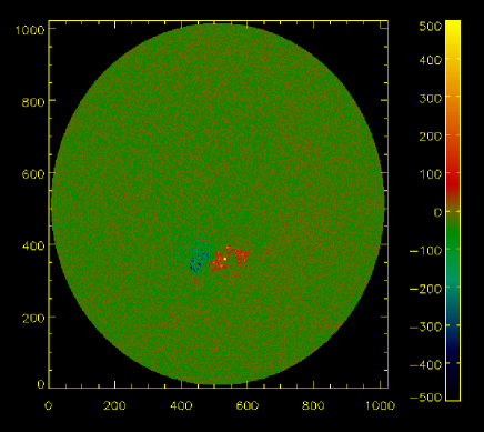
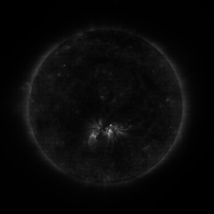
Figure 2.: Top: Full disk MDI magnetogram for 30 August 1996, bottom: Full disk EIT (wavelength171 A) image for 30 August 1996. The active region NOAA 7986 is clearly visible somewhat below the disk centre.

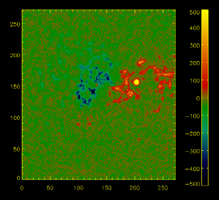
Figure 3.: Part of the full disk MDI magnetogram for 30 August 1996 with the active region extracted.

aschwanden99 applied the method of dynamic stereoscopy to the active region NOAA 7986 observed on 30 August 1996 with the EIT and MDI instruments aboard the SOHO spacecraft (see figure 2). To derive the three-dimensional loop structure on the 30 August 1996, aschwanden99 use EIT observations of the same active region taken on 29 August 1996 and 31 August 1996.

In total aschwanden99 reconstructed thirty loops, but only one loop (Loop 1 in aschwanden99) was traced along its whole length. It seems natural to choose this loop as a reference case to check the capabilities of the reconstruction method described in section 2 (e.g. iteration of $\alpha$).

For the reconstruction method we consider only a part of the full disc magnetogram close to the active region. We use Cartesian coordinates, with the $z$ axis pointing in the direction perpendicular to the photosphere. The considered area is shown in figure 3 and corresponds to the pixels $330<x<602,\quad 203<y<475$ of the full disk $1024\times 1024$ pixel MDI-image. The same region has been used in the corresponding EIT-image by aschwanden99 for the dynamic stereoscopy. This corresponds to a normalising length scale for $\alpha$ of $L=L_{x}=L_{y}=385$ Mm. The corresponding values of $\alpha$ in SI units are $|\alpha|<1.154\cdot 10^{-8}$ m^-1.

We applied both the method of minimising the distance of foot-points and the preferable method of minimising the distance of loop segments between the observed and calculated loop. In the first case we start the field line integration at one of the foot points of the observed loop, in the second case we start the field line integration at the top of the observed loop and integrate in both directions down to the photosphere ($z=0$).

Figure 4.: The functions $f(\alpha)$ (left) and $C(\alpha)$ (right) for loop 1 of aschwanden99. The function $f(\alpha)$ (foot point distance method) has a minimum at $\alpha=3.0$ and $C(\alpha)$ (loop distance method) has a minimum at $\alpha=3.5$. The rapid increase of the functions, in particular of $f(\alpha)$, for larger $\alpha$ values is caused by the rapid change of the magnetic field as the limiting value of $\alpha=\sqrt{2}\pi\simeq 4.44$ is approached.

Figure 4 shows the corresponding functions $f(\alpha)$ for the foot-point method on the left-hand side and and $C(\alpha)$ for the loop distance method on the right-hand side. The minimum of $f(\alpha)$ occurs at $\alpha=3.0$ and the minimum of $C(\alpha)$ at $\alpha=3.5$. We point out that the minimum for the $C(\alpha)$ is very flat (see right-hand side in figure 4) which means that we can expect that values of $\alpha$ which differ slightly from the minimum value will still give fits of similar quality. As the limiting value $\alpha=\sqrt{2}\pi\simeq 4.44$ is approached, both functions show a rapid increase, in particular of $f(\alpha)$. This is caused by the rapid change of the magnetic field close the limiting value of $\alpha$.

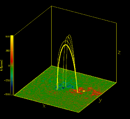
Figure 5.: Some field lines for different values of $\alpha$ and the observed loop (thick line). The $z$-axis has been stretched by a factor of $5$ to make the comparison of the observed loop and the field lines easier. In the top panel we have used the foot point distance method to determine the optimum value $\alpha=3.0$. The two other field lines shown start at the same foot point, but are for $\alpha=0.0$ and $\alpha=-2.0$. In the bottom panel the optimal value $\alpha=3.5$ has been determined by the loop distance method with starting point of integration at the loop top. The other field lines shown start at the same point but are for $\alpha=0.0$ and $\alpha=-2.0$.

Figure 5 shows the loop shape as deduced from the data (thick line) and field lines of the reconstructed coronal magnetic field for different values of $\alpha$. The top panel corresponds to the foot-point method and the bottom panel to the loop distance method. The reconstructed field-lines for the optimal values of $\alpha$ nearly coincide with the observed loops. For the foot-point method the optimal reconstructed loop is slightly higher than the observed loop. In figure 5, the $z$-axis has been stretched by a factor of $5$ to facilitate the comparison between the observed loop and the calculated field lines.

For the loop distance method one observes some deviation between observed loop and the optimal reconstructed loop at the foot-points. These deviations are slightly bigger at the left foot-point. This mismatch of the foot-points has to be balanced against the fact that the position of the observed end points of the loop is only accurate to about $10\%$ of the total observed length of the loop [Aschwanden et al. (1999)]. One also has to account for the fact that it is not clear whether the observed end points of the loop coincide with its foot points, i.e. those points where the field lines of the loop meet the photosphere.

In both cases, we also show field lines with the same starting points, but values of $\alpha$ which are different from the optimal value. It is obvious that the match between those field lines and the observed loop is not as good as that of the optimal reconstructed field.

In order to see how robust the loop distance method is with respect to changes in the integration start point of the field line used for calculating $C(\alpha)$, we have calculated $C(\alpha)$ for a grid of start points on and around the observed loop $1$ of aschwanden99. In particular, we have chosen starting points on the observed loop at $1/5$, $2/5$, $3/5$, and $4/5$ of the observed loop length plus eight further starting points at each of these distances along the loop, but at a given distance form the loop position. Four of these eight start points are located at a distance of $1/50$ of the loop length in a plane perpendicular to the local tangent of the loop. The angles between the lines connecting to neighbouring start points with the loop is $\pi/2$. The other four start points at each of the distances along the loop are arranged in the same way, but at twice the distance from the loop. Thus we have $36$ field lines and we now seek the optimum value of $\alpha$ over the complete set of field lines.

Figure 6.: The functions $C_{i}(\alpha)$ calculated for the $36$ different starting points for field line integration close to the observed loop $1$ of aschwanden99. The optimum value of $\alpha$ is around $3.0$ in this case. The lower values of $C_{i}(\alpha)$ correspond to field lines starting very close to the top of the observed loop.

The functions $C_{i}(\alpha)$, $i=1,\ldots,36$, are shown in figure 6. The optimum value of $\alpha$ derived by this method is approximately $\alpha\simeq 3.0$. The best fitting field lines all have starting points which are on or very close to the top of the observed loop. This method gives a value of $\alpha$ which is very similar to the values previously derived (within a range of $\pm 0.5$), which indicates that the exact value of the starting point for the field line integration does not influence the value of $\alpha$ very much. In particular, figure 6 shows that the minimum of all $C_{i}(\alpha)$ is relatively close to $\alpha\simeq 3.0$.

4.2 Application to multiple loops

We have so far applied the method only to one single loop. If this particular loop by chance does not represent the generic properties of the magnetic field, this may lead to a misleading value for $\alpha$ and a misrepresentation of the field. We therefore want to extend the methods described in section 2 to multiple loops. This is easily done by using the sum over several loops of either $f(\alpha)$ or $C(\alpha)$ in the minimisation process.

Table 1.: Values of $\alpha$ for all $30$ loops (loop number in first column) by aschwanden99 determined by a) applying loop distance method to each loop individually (second column, value of $C(\alpha)$ in third column), b) applying the loop distance method to groups of loops (fourth column, value of $C(\alpha)$ in fifth column), and c) applying the foot point distance method to individual loops (sixth column, value of $f(\alpha)$ seventh column).

Loop	Optimal $\alpha$	$C(\alpha)$	group $\alpha$	$C(\mbox{group}\ \alpha)$	Optimal $\alpha$	$f(\alpha)$
1	$3.5$	$0.033$	$2.5$	$0.035$	$3.0$	$0.066$
2	$2.0$	$0.026$	$2.5$	$0.027$	$2.0$	$0.048$
3	$3.0$	$0.058$	$2.5$	$0.058$	$2.0$	$0.043$
4	$2.0$	$0.076$	$2.5$	$0.076$	$2.0$	$0.017$
5	$3.0$	$0.030$	$2.5$	$0.032$	$2.0$	$0.019$
6	$3.0$	$0.027$	$2.5$	$0.030$	$2.5$	$0.015$
7	$2.5$	$0.081$	$2.5$	$0.081$	$2.5$	$0.027$
8	$1.5$	$0.312$
9	$0.5$	$0.077$	$0.0$	$0.079$	$1.0$	$0.051$
10	$2.0$	$0.280$
11	$3.0$	$0.226$
12	$-0.5$	$0.300$
13	$-1.0$	$0.048$	$-2.0$	$0.056$	$-1.0$	$0.010$
14	$-0.5$	$0.308$
15	$-1.5$	$0.261$
16	$-2.0$	$0.077$	$-2.0$	$0.077$	$-2.0$	$0.059$
17	$-2.5$	$0.064$	$-2.0$	$0.070$	$-2.5$	$0.030$
18	$-4.0$	$0.122$
19	$-1.0$	$0.228$
20	$-3.0$	$0.045$	$-2.0$	$0.051$	$-3.0$	$0.037$
21	$-1.0$	$0.043$	$-2.0$	$0.045$	$-1.5$	$0.038$
22	$-1.0$	$0.997$
23	$2.5$	$0.421$
24	$-2.0$	$0.411$
25	$-4.0$	$0.235$
26	$0.5$	$0.311$
27	$2.0$	$0.299$
28	$1.0$	$0.308$
29	$1.0$	$0.323$
30	$1.0$	$0.315$

For comparison we first apply the method described in section 4.1 to all thirty loops found by aschwanden99 individually. A list of the $\alpha$ value for each loop can be found in Table 1 together with the value $C(\alpha)$. Due to the very shallow minimum in $C(\alpha)$ and due to the uncertainties in the determination of the observed loop shapes, we only determined the $\alpha$ values in half integer steps.

aschwanden99 only traced loop $1$ fully and assumed a circular loop shape for the non-traced parts of the other loops. For some loops less than $10\%$ of their length has been traced (see Table 1 in aschwanden99). Certainly force free loops will usually not be circular, and if the ad hoc assumption of circular loop shapes is wrong for a poorly traced loop, one cannot expect a satisfactory a agreement with the results of our method. However, since in the present paper we are mainly interested in testing our method we have therefore included the results for poorly traced loops in Table 1. We considered values of $C<0.1$ (in the normalisation used) as small enough, because checking the fits to the observed loops still gave acceptable results for this value. The values of $\alpha$ for all other loops have to be regarded with caution.

In this sense, we are able to fit $13$ of the $30$ loops with reasonable accuracy, as indicated by relatively small values of the individual $C(\alpha)$. We emphasize that our assumption of linear force-free fields may also be too restrictive for some loops. This once more indicates the necessity to extend the method to nonlinear force free fields.

The results for the individual loops indicate that two basic subgroups of loops can be identified, namely the loops 1-7 (subgroup 1) which all have positive values of $\alpha$ and the loops $13,16,17,20,21$ (subgroup 2) which have negative values of $\alpha$. Subgroup 2 contains only loops for which only a very small part of the total loop has been observed so that the circular extension is only determined by an almost straight line. It is therefore doubtful whether the derived $\alpha$ values are really meaningful for subgroup 2. Since we are mainly interested in testing the method in this paper, we have nevertheless included the results for subgroup 2, but the results are more interesting from a methodological point-of-view. A difference between the two subgroups is their inclination angle with the direction perpendicular to the solar surface (see figure 7).

In addition we notice that loop 9 is nearly potential and belongs to neither of these subgroups. We point out that for these loops the foot-point method and the loop distance method lead to similar optimal values of $\alpha$ as can be seen by comparing the first and the last two rows of Table 1.

To assess the possible differences between fitting single loops and groups of several loops, we minimised the sum of the individual $C$’s over the loop subgroups, $C(\alpha)=C_{1}(\alpha)+C_{2}(\alpha)+\dots$, $i=$ loop number, for both subgroups identified above. As the loops in the two subgroups are individually fitted best by $\alpha$ values with opposite sign, it does not make sense to try and fit both groups simultaneously. This is an obvious limitation of the method imposed by the linear force-free field extrapolation which can only be overcome by non-linear force-free field extrapolation allowing for a spatial variation of $\alpha$.

We found the optimal values of $\alpha=2.5$ for subgroup 1 and $\alpha=-2.0$ for subgroup 2. As in the individual cases the sign of $\alpha$ for the two loop subgroups is different. The value of $\alpha$ for subgroup 1 is slightly lower than the average value of the optimal $\alpha$ for that subgroup ($\bar{\alpha}\approx 2.7$). For the second subgroup, the optimal value of $\alpha$ has to be compared to an average of the individual values of $\bar{\alpha}\approx-1.9$.

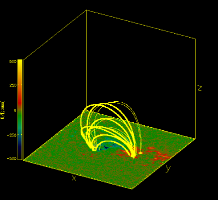
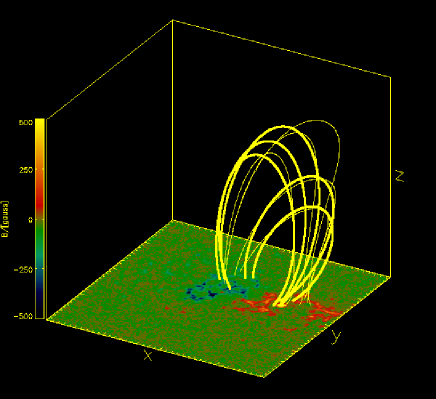
Figure 7.: Upper panel: loops 1-7 and fitted magnetic field lines for $\alpha=2.5$. Lower panel: loops 13,16,17,20,21 and fitted magnetic field lines for $\alpha=-2.0$

The values of $C_{i}(\alpha)$ for the optimal group $\alpha$ for each loop in a group are only slightly larger (about $5-10\%$) than the optimal values for single loop optimisation. We therefore conclude that the magnetic field close to subgroup 1 can be represented with a reasonable accuracy by a linear force-free field with $\alpha=2.5$ and the field of subgroup 2 by $\alpha=-2.0$. A three-dimensional view of the loops and the fitted field lines is shown in figure 7 where the upper panel corresponds to subgroup 1 and the lower panel to subgroup 2. The observed loops are indicated by thick lines and the optimised reconstructed field lines by thin lines.

As can be clearly seen in figure 7 the main difference between the loops in the two subgroups is that all loops in subgroup 1 have a negative inclination angle with the vertical whereas all loops in subgroup 2 have a positive inclination angle (see also Table 1 in aschwanden99). As shown above this corresponds to a positive value of $\alpha$ for subgroup 1 and a negative $\alpha$ for subgroup 2. Figure 7 also shows that the two subgroups occupy different spatial regions although their foot points are generally not too far apart.

We would like to emphasize again that all the results presented in this section depend on the circular loop extrapolation used by aschwanden99. Therefore all derived $\alpha$ values can be considered only as accurate as the shape of the corresponding loop used for the determination of $\alpha$. In particular, extrapolations based only on small observed parts of loops have to be regarded with great caution. However, we were mainly interested in testing our method and under the assumption that the extrapolated loops are correct, the method seems to give consistent results.

5 Conclusions and Outlook

In this paper we undertook a first step towards including three-dimensional information from stereoscopic observations into a reconstruction of coronal magnetic fields from photospheric magnetic field measurements. Due to the low plasma $\beta$ in the solar corona force-free magnetic fields can be used and in the present paper, we restricted our analysis to linear force-free fields for simplicity. The extrapolation method uses the line-of-sight photospheric magnetic field as a boundary condition.

As the coronal plasma has a very high conductivity, the magnetic field is frozen into the plasma. Therefore one can assume that the coronal plasma structures also outline the magnetic field. This is the fundamental assumption of our method. The idea of our reconstruction method is to take both the photospheric magnetogram and the three-dimensional stereoscopic information into account to derive the magnetic field configuration in the solar corona. The magnetogram provides information regarding the strength and the distribution of the magnetic fields, whereas the three-dimensional loop shapes restrict the current density. The method works iteratively in that we first calculate a magnetic field configuration from the line of sight magnetogram for a given value of $\alpha$ without considering the stereoscopic information. To test the configuration we compare a magnetic loop of this magnetic field with the stereoscopic observations. This can be done in various ways of which we have presented two (foot-point method and loop distance method). The value of $\alpha$ is then systematically optimised by minimising the difference between the observed and the reconstructed loop shape.

We have applied this method to loops deduced by aschwanden99 using the method of dynamic stereoscopy for the active region NOAA 7986 observed with SOHO/MDI and EIT on 1996 August 30. For the future we are planing to apply our method to data taken by the SECCHI instrument aboard the STEREO mission.

The results obtained for the aschwanden99 data are promising, but indicate the need for improving the method further by the use of non-linear force-free fields. Work along these lines is in progress and will be presented in a forthcoming publication.

We thank Bernd Inhester, Fabrice Portier-Fozzani, Eric Priest and Rainer Schwenn for useful discussions. We also thank the referee for insightful comments. The data used have been provided by the SOHO/MDI and SOHO/EIT Consortia. SOHO is a joint ESA/NASA program. This work was supported by an EC Marie-Curie-Fellowship (TW) and a PPARC Advanced Fellowship (TN).

References

- Alissandrakis (1981) Alissandrakis, C.E.: 1981, Astron. Astrophys. 100, 197.
- Amari et al. (1997) Amari, T., Aly, J.J., Luciani, J.F., Boulmezaoud, T.Z., Mikic, Z.: 1997, Solar Phys. 174, 129.
- Aschwanden et al. (1999) Aschwanden, M.J., Newmark, J.S., Delaboudiniere,J-P., Neupert, W.M., Klimchuk, J.A., Gary, G.A., Portier-Fozzani, F., Zucker, A.: 1999, Astrophys. J. 515, 842.
- Chiu and Hilton (1977) Chiu, Y.T., Hilton, H.H.: 1977, Astrophys. J. 212, 821.
- Gary (1989) Gary, G.A.: 1989, Astrophys. J. Suppl. 69, 323.
- Golub and Pasachoff (1997) Golub, L. and Pasachoff, J.M.: 1997, The Solar Corona, Cambridge University Press, Cambridge, p. 167.
- Lothian and Browning (1995) Lothian, R.M. and Browning, P.K.: 1995, Solar Phys. 161, 289.
- McClymont, Jiao, and Mikic (1997) McClymont, A.N., Jiao, L., Mikic, Z.: 1997, Solar Phys. 174, 191.
- Nakagawa and Raadu (1972) Nakagawa, Y. and Raadu, M.A.: 1972, Solar Phys. 25, 127.
- Petrie and Neukirch (2000) Petrie, G.J.D. and Neukirch, T.: 2000, Astron. Astrophys. 356, 735.
- Pevtsov, Canfield, and Metcalf (1995) Pevtsov, A.A., Canfield, R.C., and Metcalf, T.R.: 1995, Astrophys. J. 440, L109.
- Rädler (1974) Rädler, K.-H.: 1974, Astron. Nachr. 295, 73.
- Roumeliotis (1996) Roumeliotis, G.: 1996, Astrophys. J. 473, 1095.
- Rudenko (2001a) Rudenko, G.V.: 2001a, Solar Phys. 198, 5.
- Rudenko (2001b) Rudenko, G.V.: 2001b, Solar Phys. 198, 279.
- Sakurai (1981) Sakurai, T.: 1981, Solar Phys. 69, 343.
- Sakurai (1982) Sakurai, T.: 1982, Solar Phys. 76, 301.
- Schatten, Wilcox, and Ness (1969) Schatten, K.H., Wilcox, J.M., and Ness N.F.: 1969, Solar Phys. 6, 442.
- Schmidt (1964) Schmidt, H.V.: 1964 in W.N. Ness (ed.), ASS-NASA Symposium on the Physics of Solar Flares, NASA SP-50, p. 107.
- Seehafer (1978) Seehafer, N.: 1978, Solar Phys., 58, 215.
- Seehafer (1982) Seehafer, N.: 1982, Solar Phys., 81, 69.
- Semel (1967) Semel, M.: 1967, Ann. Astrophys. 30, 513.
- Semel (1988) Semel, M.: 1988, Astron. Astrophys. 198, 293.
- Wheatland (1999) Wheatland, M.S.: 1999, Astrophys. J. 518, 948.
- Wheatland, Sturrock, and Roumeliotis (2000) Wheatland, M.S., Sturrock, P.A., and Roumeliotis, G.: 2000, Astrophys. J. 540, 1150.
- Wu, Chang, and Hagyard (1985) Wu, S.T., Chang, H.M., Hagyard, M.J.: 1985, in M.J. Hagyard (ed.), Measurements of Solar Magnetic Fields, NASA CP-2374, p. 17.
- Yan and Sakurai (2000) Yan, Y. and Sakurai, T.: 2000, Solar Phys. 195, 89.
- Zhao and Hoeksema (1993) Zhao, X. and Hoeksema, J.T.: 1993, Solar Phys. 143, 41.
- Zhao and Hoeksema (1994) Zhao, X. and Hoeksema, J.T.: 1994, Solar Phys. 151, 91.
- Zhao, Hoeksema, and Scherrer (2000) Zhao, X., Hoeksema, J.T., and Scherrer, P.H.: 2000, Astrophys. J. 538, 932.