11email: belloche,kmenten,ccomito,schilke,sthorwirth,chieret@mpifr-bonn.mpg.de 22institutetext: I. Physikalisches Institut, Universität zu Köln, Zülpicher Str. 77, D-50937 Köln, Germany
22email: hspm@ph1.uni-koeln.de 33institutetext: National Radio Astronomy Observatory, 520 Edgemont Road, Charlottesville, VA 22903-2475, USA
33email: jott@nrao.edu 44institutetext: California Institute of Technology, 1200 E. California Blvd., Caltech Astronomy, 105-24, Pasadena, CA 91125-2400, USA 55institutetext: CSIRO Australia Telescope National Facility, Cnr Vimiera Pembroke Roads, Marsfield NSW 2122, Australia
Detection of amino acetonitrile in Sgr B2(N) ††thanks: Based on observations carried out with the IRAM Plateau de Bure Interferometer, the IRAM 30m telescope, the Australia Telescope Compact Array, and the NRAO Very Large Array. IRAM is supported by INSU/CNRS (France), MPG (Germany) and IGN (Spain). The Australia Telescope Compact Array is part of the Australia Telescope which is funded by the Commonwealth of Australia for operation as a National Facility managed by CSIRO. The National Radio Astronomy Observatory is a facility of the National Science Foundation operated under cooperative agreement by Associated Universities, Inc.
Abstract
Context. Amino acids are building blocks of proteins and therefore key ingredients for the origin of life. The simplest amino acid, glycine (NH2CH2COOH), has long been searched for in the interstellar medium but has not been unambiguously detected so far. At the same time, more and more complex molecules have been newly found toward the prolific Galactic center source Sagittarius B2.
Aims. Since the search for glycine has turned out to be extremely difficult, we aimed at detecting a chemically related species (possibly a direct precursor), amino acetonitrile (NH2CH2CN).
Methods. With the IRAM 30m telescope we carried out a complete line survey of the hot core regions Sgr B2(N) and (M) in the 3 mm range, plus partial surveys at 2 and 1.3 mm. We analyzed our 30m line survey in the LTE approximation and modeled the emission of all known molecules simultaneously. We identified spectral features at the frequencies predicted for amino acetonitrile lines having intensities compatible with a unique rotation temperature. We also used the Very Large Array to look for cold, extended emission from amino acetonitrile.
Results. We detected amino acetonitrile in Sgr B2(N) in our 30m telescope line survey and conducted confirmatory observations of selected lines with the IRAM Plateau de Bure and the Australia Telescope Compact Array interferometers. The emission arises from a known hot core, the Large Molecule Heimat, and is compact with a source diameter of 2 (0.08 pc). We derived a column density of cm-2, a temperature of 100 K, and a linewidth of 7 km s-1. Based on the simultaneously observed continuum emission, we calculated a density of cm-3, a mass of 2340 M⊙, and an amino acetonitrile fractional abundance of . The high abundance and temperature may indicate that amino acetonitrile is formed by grain surface chemistry. We did not detect any hot, compact amino acetonitrile emission toward Sgr B2(M) or any cold, extended emission toward Sgr B2, with column-density upper limits of and cm-2, respectively.
Conclusions. Based on our amino acetonitrile detection toward Sgr B2(N) and a comparison to the pair methylcyanide/acetic acid both detected in this source, we suggest that the column density of both glycine conformers in Sgr B2(N) is well below the best upper limits published recently by other authors, and probably below the confusion limit in the 1-3 mm range.
Key Words.:
Astrobiology – Astrochemistry – Line: identification – Stars: formation – ISM: individual objects: Sagittarius B2 – ISM: molecules1 Introduction – general methods
Among the still growing list of complex molecules found in the interstellar medium, so-called “bio”molecules garner special attention. In particular, the quest for interstellar amino acids, building blocks of proteins, has engaged radio and millimeter wavelength astronomers for a long time. Numerous published and unpublished searches have been made for interstellar glycine, the simplest amino acid (Brown et al. 1979; Hollis et al. 1980; Berulis et al. 1985; Combes et al 1996; Ceccarelli et al. 2000; Hollis et al. 2003; Jones et al. 2007; Cunningham et al. 2007). Its recent “detection” claimed by Kuan et al. (2003) has been persuasively rebutted by Snyder et al. (2005). Since the early days of molecular radio astronomy, Sagittarius B2 has been a favorite target in searches for complex molecules in space.
1.1 The target: Sagittarius B2
Sagittarius B2 (hereafter Sgr B2 for short) is a very massive (several million solar masses) and extremely active region of high-mass star formation at a projected distance of pc from the Galactic center. Its distance from the Sun is assumed to be the same as the Galactic center distance, . Reid (1993), reviewing various methods to determine , arrived at a “best estimate” of 8.0 0.5 kpc, a value that we adopt in this article. It is supported by recent modeling of trajectories of stars orbiting the central black hole, which yields 7.94 0.42 kpc (Eisenhauer et al. 2003).
There are two major centers of activity, Sgr~B2(M) and Sgr~B2(N) separated by pc. In each of them, recent star formation manifests itself in a multitude of Hii regions of many sizes, from hypercompact to compact (Gaume et al. 1995), and there is abundant material to form new stars evident by massive sources of molecular line and submillimeter continuum emission from dust (Lis et al. 1991, 1993).
1.1.1 Sgr B2 as part of the Central Molecular Zone
Some of the first detections of interstellar organic molecules (at cm-wavelengths!) were made toward Sgr B2 (see Menten 2004 for a historical perspective). The low intrinsic line strengths make these cm lines unlikely candidates for detection. However, the situation is helped, first, by the fact that many of the transitions in question may have inverted levels (Menten 2004) and amplify background radio continuum emission which is very intense at cm wavelengths (Hollis et al. 2007). Second, the spatial distributions of many species are characterized by spatially extended emission covering areas beyond Sgr B2 itself, filling single dish telescope beams, thus producing appreciable intensity even when observed with low spatial resolution (Cummins, Linke, & Thaddeus 1986; Jones et al. 2008). This emission is characterized by low rotation temperatures, favoring lower frequency lines. Recent identifications of “new” species include glycolaldehyde CH2OHCHO (Hollis et al. 2000, 2001), ethylene glycol HOCH2CH2OH (Hollis et al. 2002), and vinyl alcohol CH2CHOH (Turner & Apponi 2001).
Sgr B2 and its surroundings are part of the Central Molecular Zone (CMZ) of our Galaxy, a latitude wide band stretching around the Galactic center from longitude to (see, e.g., Morris & Serabyn 1996). The CMZ contains spatially extended emission of many complex organic molecules (Minh et al. 1992; Dahmen et al. 1997; Menten 2004; Requena-Torres et al. 2006).
1.1.2 The Large Molecule Heimat
Near Sgr B2(N), there is a hot, dense compact source that has a mm-wavelength line density second to no other known object. This source, for which Snyder, Kuan, & Miao (1994) coined the name “Large Molecule Heimat” (LMH), is characterized by very high densities ( cm-3) and gas temperatures ( K). In recent years arcsecond resolution interferometry with the BIMA array has resulted in the detection and imaging of increasingly complex organic species toward the LMH, such as vinyl cyanide CH2CHCN, methyl formate HCOOCH3, and ethyl cyanide CH3CH2CN (Miao et al. 1995; Miao & Snyder 1997), formamide NH2CHO, isocyanic acid HNCO, and methyl formate HCOOCH3 (Kuan & Snyder 1996), acetic acid CH3COOH (Mehringer et al. 1997; Remijan et al. 2002), formic acid HCOOH (Liu et al. 2001), and acetone (CH3)2CO (Snyder et al. 2002). All the interferometric observations are consistent with a compact (few arcsec diameter) source that had already been identified as the source of high-density-tracing non-metastable ammonia line emission by Vogel et al. (1987) and thermal methanol emission by Mehringer & Menten (1997 , their source “i”). The LMH also hosts a powerful H2O maser region (Reid et al. 1988), which provides evidence that it is very young (see Sect. 4.1).
1.2 The complex spectra of complex molecules
Complex molecules in general have large partition functions, in particular for the elevated temperatures ( K) in molecular hot cores, dense and compact cloud condensations internally heated by a deeply embedded, young high-mass (proto)stellar object. Therefore, most individual spectral lines are weak and might easily get hidden in the “line forest” found toward these frequently extremely line-rich sources. To a large part, this forest consists of rotational lines, many of them presently unidentifiable, from within relatively low-lying vibrational states of molecules. Most of the candidate molecules from which these lines originate are known to exist in these sources, but laboratory spectroscopy is presently lacking for lines from the states in question. At this point in the game, unequivocally identifying a species in a spectrum of a hot core covering a wide spectral range requires the following steps: as described in detail in Sect. 3.2, assuming Local Thermodynamic Equilibrium (LTE) (which applies at the high densities in hot cores) a model spectrum is calculated for an assumed rotation temperature, column density, line width and other parameters. This predicts lines of a given intensity at all the known frequencies. Then at least two conditions have to be fulfilled: (i) All predicted lines should have a counterpart in the observed spectrum with the right intensity and width – no single line should be missing. (ii) Follow-up observations with interferometers have to prove whether all lines from the candidate species are emitted from the same spot. Given the chemical variety in hot core regions, this is a powerful constraint. Moreover, interferometer images tend to have less line confusion, since many lines that are blended in larger beam single-dish spectra arise from different locations or are emitted by an extended region that is spatially filtered out. Using an interferometer for aiding molecule identifications was pioneered by L. Snyder and collaborators who (mostly) used the Berkeley-Illinois-Maryland-Array (BIMA) to clearly identify a number of species in the Sgr B2(N) Large Molecule Heimat (see Sect. 1.1.2).
We carried out a complete line survey of the hot core regions Sgr B2(N) and (M) with the IRAM 30m telescope at 3 mm, along with partial surveys at 2 and 1.3 mm. One of the overall goals of our survey was to better characterize the molecular content of both regions. It also allows searches for “new” species once we have identified the lines emitted by known molecules (including vibrationally and torsionally excited states). In particular, many complex molecules have enough lines in the covered frequency ranges to apply criterion (i) above. Once a species fulfils this criterion, interferometer measurements of selected lines can be made to check criterion (ii).
1.3 Amino acetonitrile
One of our target molecules was amino acetonitrile (NH2CH2CN), a molecule chemically related to glycine. Whether it is a precursor to the latter is under debate (see Sect. 4.3). Not many astronomical searches for amino acetonitrile have been reported in the literature. In his dissertation, Storey (1976) reported searches for the and transitions at 1350.5 and 9071.7 MHz, respectively with the Parkes 64 m telescope. On afterthought, the only chance of success for their observations would have been if amino acetonitrile existed on large spatial scales, similar to the molecules described in Sect. 1.1.1 (see Sect. 3.7 for further limits on extended amino acetonitrile emission). Recently, Wirström et al. (2007) reported unsuccessful searches of a number of mm-wavelength transitions of amino acetonitrile toward a number of hot cores.
Here, we report our detection of warm compact emission from amino acetonitrile in Sgr B2(N) with the IRAM 30m telescope, the Plateau de Bure Interferometer (PdBI) and the Australia Telescope Compact Array (ATCA), and upper limits on cold, spatially extended emission from amino acetonitrile that we obtained with the NRAO Very Large Array (VLA). Section 2 summarizes the observational details. We present our results in Sect. 3. Implications in terms of interstellar chemistry are discussed in Sect. 4. Our conclusions are summarized in Sect. 5.
2 Observations and data reduction
2.1 Single-dish observations and data reduction
We carried out millimeter line observations with the IRAM 30m telescope on Pico Veleta, Spain, in January 2004, September 2004 and January 2005. We used four SIS heterodyne receivers simultaneously, two in the 3 mm window connected to the autocorrelation spectrometer VESPA and two in the 1.3 mm window with filter banks as backends. A few selected frequency ranges were also observed with one SIS receiver at 2 mm in January 2004. The channel spacing and bandwidth were 0.313 and 420 MHz for each receiver at 3 and 2 mm, and 1 and 512 MHz for each receiver at 1.3 mm, respectively. The observations were done in single-sideband mode with sideband rejections of –3 at 3 mm, –7 at 2 mm, and –8 at 1.3 mm. The half-power beamwidths can be computed with the equation HPBW () = . The forward efficiencies were 0.95 at 3 mm, 0.93 at 2 mm, and 0.91 at 1.3 mm, respectively. The main-beam efficiencies were computed using the Ruze function , with , , and the wavelength in mm (see the IRAM 30m telescope system summary on http:www.iram.es). The system temperatures ranged from 96 to 600 K at 3 mm, from 220 to 720 K at 2 mm (except at 176 GHz where they ranged from 2400 to 3000 K), and from 280 to 1200 K at 1.3 mm. The telescope pointing was checked every hours on Mercury, Mars, 1757240 or G10.62, and found to be accurate to 2–3 (rms). The telescope focus was optimized on Mercury, Jupiter, Mars or G34.3+0.2 every –3 hours. The observations were performed toward both sources Sgr B2(N) (=17h47m200, =2219.0, = 64 km s-1) and Sgr B2(M) (=17h47m204, =2307.0, = 62 km s-1) in position-switching mode with a reference position offset by (,)=(,) with respect to the former. The emission toward this reference position was found to be weak: (12CO 10) 2 K, (CS 21) 0.05 K, (12CO 21) 1.5 K, (13CO 21) 0.1 K, and it is negligible for higher excitation lines and/or complex species.
We observed the full 3 mm window between 80 and 116 GHz toward both sources. The step between two adjacent tuning frequencies was 395 MHz, which yielded an overlap of 50 MHz. The autocorrelator VESPA produces artificial spikes with a width of 3–5 channels at the junction between subbands (typically 2 or 3 spikes per spectrum). To get rid of these artefacts, half of the integration time at each tuning frequency was spent with the backend shifted by 50 MHz, so that we could, without any loss of information, systematically remove in each spectrum 5 channels at each of the 6 junctions between subbands that were possibly affected by this phenomenon. At 2 mm, we observed at only 8 selected frequencies, and removed the artificial spikes in the same way as at 3 mm. At 1 mm, we covered the frequency ranges 201.8 to 204.6 GHz and 205.0 to 217.7 GHz, plus a number of selected spots at higher frequency. For each individual spectrum, we removed a 0th-order (constant) baseline by selecting a group of channels which seemed to be free of emission or absorption. However, many spectra are full of lines, especially at 1.3 mm where we reached the confusion limit, and we may have overestimated the level of the baseline for some of them.
In scale, the rms noise level achieved towards Sgr B2(N) is about 15–20 mK below 100 GHz, 20–30 mK between 100 and 114.5 GHz, and about 50 mK between 114.5 and 116 GHz. At 1.3 mm, we reached the confusion limit for most of the spectra. The data were reduced with the CLASS software, which is part of the GILDAS software package (see http://www.iram.fr/IRAMFR/GILDAS).
2.2 Interferometric observations with the PdBI
We observed Sgr B2(N) with the PdBI for 4.7 hours on February 7th, 2006 with 6 antennas in the high-resolution configuration (E24E68E04N46W27N29). The coordinates of the phase center were , . The 3 and 1.2 mm receivers were tuned to 81.982 and 245.380 GHz, respectively, in single side band mode. At 3 mm, there were two spectral windows centered at 81.736 and 82.228 GHz with a bandwidth of 80 MHz and a channel separation of 0.313 MHz, and two continuum windows of 320 MHz bandwidth centered at 81.852 and 82.112 GHz. The atmospheric phase stability was good for the 3 mm band but bad for the 1.2 mm band. Therefore we do not analyze the 1.2 mm data. The system temperatures were typically 150–220 K at 3 mm in the lower sideband. The (naturally-weighted) synthesized half-power beam width was with P.A. 10∘, and the primary beam was FWHM. The correlator bandpass was calibrated on the quasar 3C 273. Phase calibration was determined on the nearby sources NRAO 530 and 1622297. The time-dependent amplitude calibration was done on 1622297, NRAO 530, 1334127, and 1749096, while the absolute flux density scale was derived from MWC 349. The absolute calibration uncertainty is estimated to be 15. The data were calibrated and imaged using the GILDAS software. The continuum emission was estimated on line-free portions of the bands and removed in the uv plane. The deconvolution was performed with the CLEAN method (Clark 1980).
2.3 Interferometric observations with the ATCA
We observed Sgr B2(N) with the ATCA on May 17th, 2006 in the hybrid H 214 configuration for 6 hours, for 7 hours on July 30th, 2006 in the H 168 configuration, and for 6 hours in the compact H 75 configuration on September 25th, 2006. The coordinates of the phase center were , . The 3 mm receiver was alternately tuned to three frequency pairs of 90.550 and 93.200 GHz, 90.779 and 93.200 GHz, and 99.978 and 97.378 GHz in single side band mode, where only the first frequency of each pair was in spectral line mode with 32 MHz bandwidth and 128 channels. The second frequency of each pair was configured for continuum observations with 128 MHz bandwidth each. The system temperatures were typically 60 K. The (naturally-weighted) synthesized half-power beam width was with P.A. for H 214, with P.A. for H 168, and with P.A. for H 75. The combination of H 214 and H 168 yields a synthesized half-power beam width of with P.A. , and the combination of all three configurations a synthesized half-power beam width of with P.A. . The primary beam was FWHM. The correlator bandpass was calibrated on PKS 1253055. The phase and gain calibration was determined on the nearby source PKS 175939. The absolute flux density scale was derived from Uranus. The absolute calibration uncertainty is estimated to be 20. The data were calibrated, continuum subtracted, imaged, and deconvolved using the software package MIRIAD (Sault et al. 1995).
Our ATCA data are affected by two problems. First, the tuning frequency used in May was not updated for the new observatory velocity in July and September. As a result, the observed bands were shifted by +12 and +16 MHz in rest frequency in the H 168 and H 75 configurations with respect to the H 214 configuration. Second, we suspect a technical problem with the tuning at 99 GHz in May and July because we do not detect any line in the H 214 and H 168 configurations while we easily detect two lines in the H 75 configuration: one unidentified line and one line from CH3CH3CO, vt=1 according to our line survey with the IRAM 30m telescope. Comparing this band to the two other bands where we detect every line in each configuration (albeit with different intensities due to variable spatial filtering), we consider it to be very unlikely that the two lines detected at 99 GHz in the H 75 configuration are completely filtered out in the H 214 and H 168 configurations. Since the amino acetonitrile transition is shifted out of the H 75 band at 99 GHz (due to the variation of the observatory velocity), we do not analyze this dataset in the present article.
2.4 Interferometric observations with the VLA
We used the NRAO Very Large Array to search for the multiplet of amino acetonitrile at 9071.208 MHz and examine the possibility of cold extended emission from this molecule. The VLA data were taken over a 1.5 h interval on February 13th, 2003 when the array was in its lowest-resolution () configuration. Three minute long scans of the following position in Sgr B2 were alternated with scans of the phase calibrator NRAO 530. For absolute flux density calibration, 3C286 was observed. Our phase center in Sgr B2 was at =17h47m2000, =2251.0. This is South and North of our 30m telescope pointing positions for Sgr B2(N) and (M), respectively.
Our observations were done in spectral line mode with one intermediate frequency (IF) band split into 32 channels, each of which had a width of 0.1953 MHz, corresponding to 6.46 km s-1. The usable central 72 frequency range of the IF bandwidth, 4.49 MHz, covered all the multiplet’s 7 hyperfine structure (hfs) components111The multiplet consists of 9 hyperfine components with significant intensity spanning the frequency range from 9070.233 to 9073.867 MHz. Twice two components have basically the same frequency (difference of about 0.1 kHz) so that under favorable conditions there are 7 hyperfine lines observable. Full spectroscopic information for amino acetonitrile can be found in the CDMS (entry 56507).. This frequency range corresponds to a total velocity coverage of 148 km s-1. The center velocity was set to Vlsr = 65 km s-1. A 4.49 MHz bandwidth “pseudo continuum” database (the so-called “channel 0”) was created by averaging the central 23 channels. The -data were calibrated using the NRAO’s Astronomical Imaging Processing System (AIPS). Several iterations of self calibration delivered a high quality continuum image. Using UVLIN, the average of selected regions of the line -database were subtracted channel by channel from the latter to remove the continuum level. To calibrate the spectral line data, the phase and amplitude corrections determined by the initial calibration, as well as by the self calibration were transferred to the line database and applied to them successively, producing a 23 channel database which was imaged channel by channel using natural weighting. The synthesized beam width of the images is FWHM with a position angle of East of North222The calibrated and deconvolved data cubes and images (line and continuum) obtained with the PdBI, the ATCA, and the VLA are available in FITS format at the CDS via anonymous ftp to cdsarc.u-strasbg.fr (130.79.128.5) or via http://cdsweb.u-strasbg.fr/cgi-bin/qcat?J/A+A/..
3 Identification of amino acetonitrile
3.1 Amino acetonitrile frequencies
| Parameter | Value | |
|---|---|---|
| 30 246 | .456 1 (71) | |
| 4 761 | .061 02 (84) | |
| 4 310 | .751 23 (76) | |
| 676 | .62 (99) | |
| 55 | .298 6 (69) | |
| 3 | .068 53 (68) | |
| 671 | .60 (40) | |
| 28 | .893 (106) | |
| 30 | .b | |
| 2 | .686 1 (268) | |
| 120 | .1 (72) | |
| 9 | .593 (276) | |
| 2 | .989 (225) | |
-
Watson’s -reduction was employed in the representation . The dimensionless weighted rms of the fit is 0.51, therefore, the numbers in parentheses may be considered as two standard deviations in units of the least significant figures.
-
Assumed value (see Sect. 3.1).
In the course of the present investigation an amino acetonitrile entry (tag: 56507) has been prepared for the catalog of the Cologne Database for Molecular Spectroscopy (CDMS, see Müller et al. 2001, 2005). The laboratory transition frequencies were summarized by Bogey, Dubus, & Guillemin (1990). Their work included microwave transitions reported without 14N quadrupole splitting by MacDonald & Tyler (1972), Pickett (1973), as well as microwave transitions reported with quadrupole splitting by Brown et al. (1977); the latter data were used with the reported splitting. Line fitting and prediction of transition frequencies was done with the SPFIT/SPCAT suite of programs (Pickett 1991) using a Watson type Hamiltonian in the reduction in the representation (see, e.g., Gordy & Cook 1984).
The set of spectroscopic parameters reported by Bogey et al. (1990) included terms of up to decic order (), rather unusual for an apparently rigid and fairly heavy molecule, and we found the higher order parameters to be surprisingly large. Moreover, the off-diagonal sextic distortion parameter was larger in magnitude than , and was not even used in the fit; the importance of these parameters is reversed to what is more commonly found. Therefore, we performed a trial fit with the octic and decic parameters as well as and omitted and the sextic term fixed to a value that was estimated from . Subsequently, we found that inclusion of improved the quality of the fit. All transitions but five having and could be reproduced well. Two of these had and deviated MHz from the predicted frequencies which was only twice the predicted uncertainty. The inclusion of these transitions in the fit caused relatively small changes in and ; changes in the remaining parameters were within the uncertainties. Therefore, it is likely that the assignments of these two transitions are correct. Effects on the predicted transition frequencies are negligible. The remaining three transitions are considered to be mis-assignments as their inclusion would require many more higher order distortion parameters with apparently unphysical values and a poorer quality of the fit. Hence, those transitions were omitted from our fit. The resulting spectroscopic parameters are given in Table 1. The rotational partition function at 75 and 150 K is 4403 and 12460, respectively.
3.2 Modeling of the 30m line survey
The average line density above 3 in our 30m survey is about 100 and 25 features per GHz for Sgr B2(N) and (M), respectively, translating into about 3700 and 950 lines over the whole 80–116 GHz band. To identify a new molecule in such a line forest and reduce the risk of mis-assignments, it is essential to model first the emission of all known molecules, including vibrationally and torsionally excited states, and their isotopologues. We used the XCLASS software (see Comito et al. 2005 and references therein) to model the emission and absorption lines in the LTE approximation. These calculations take into account the beam dilution, the line opacity, and the line blending. The molecular spectroscopic parameters are taken from our line catalog which contains all entries from the CDMS catalog (Müller et al. 2001, 2005) and from the molecular spectroscopic database of the Jet Propulsion Laboratory (JPL, see Pickett et al. 1998), plus additional “private” entries.
Each molecule is modeled separately with the following set of input parameters: source size, rotational temperature, column density, velocity linewidth, velocity offset with respect to the systemic velocity of the source, and a flag indicating if it is an emission or absorption component. For some of the molecules, it was necessary to include several velocity components to reproduce the observed spectra. The velocity components in emission are supposed to be non-interacting, i.e. the intensities add up linearly. The radiative transfer is computed in the following way: first the emission line spectrum is calculated, and then the absorption lines, using the full (lines + continuum) emission spectrum as background to absorb against. The vibrationally and/or torsionally excited states of some molecules were modeled separately from the ground state. The input parameters were varied until a good fit to the data was obtained for each molecule. The whole spectrum including all the identified molecules was then computed at once, and the parameters for each molecule were adjusted again when necessary. The quality of the fit was checked by eye over the whole frequency coverage of the line survey. We favored our eye-checking method against an automated fitting because the high occurence of line blending and the uncertainty in the baseline removal would in many cases make an automated fitting procedure fail.
The detailed results of this modeling will be published in a forthcoming article describing the complete survey (Belloche et al., in prep). So far, we have identified 51 different molecules, 60 isotopologues, and 41 vibrationally/torsionally excited states in Sgr B2(N), which represent about 60 of the lines detected above the 3 level. In Sgr B2(M), the corresponding numbers are 41, 50, 20, and 50, respectively.
3.3 Detection of amino acetonitrile with the 30m telescope
| Na | Transitionb | Frequency | Unc.c | Eld | S | Comments | |
|---|---|---|---|---|---|---|---|
| (MHz) | (kHz) | (K) | (D2) | (mK) | |||
| (1) | (2) | (3) | (4) | (5) | (6) | (7) | (8) |
| 1 | 90,9 - 80,8 | 80947.479 | 7 | 16 | 60 | 33 | Detected |
| 2 | 92,8 - 82,7 | 81535.184 | 6 | 21 | 57 | 18 | Strong HC13CCN, v=0 |
| 3 | 95,5 - 85,4⋆ | 81700.966 | 6 | 47 | 41 | 13 | Group detected, partial blend with U-line |
| 5 | 96,3 - 86,2⋆ | 81702.498 | 5 | 60 | 33 | 13 | Group detected, partial blend with U-line |
| 7 | 94,6 - 84,5⋆ | 81709.838 | 6 | 35 | 48 | 13 | Group detected |
| 9 | 97,3 - 87,2 | 81709.848 | 6 | 76 | 24 | 13 | Group detected |
| 10 | 94,5 - 84,4 | 81710.098 | 6 | 35 | 48 | 13 | Group detected |
| 11 | 93,7 - 83,6 | 81733.892 | 6 | 27 | 53 | 13 | Detected, blend with CH3OCH3 and HCC13CN, v6=1 |
| 12 | 93,6 - 83,5 | 81756.174 | 6 | 27 | 53 | 13 | Detected, blend with U-line |
| 13 | 92,7 - 82,6 | 82224.644 | 7 | 21 | 57 | 19 | Detected, uncertain baseline |
| 14 | 91,8 - 81,7 | 83480.894 | 8 | 17 | 59 | 17 | Blend with C2H3CN, v=0 |
| 15 | 101,10 - 91,9 | 88240.541 | 8 | 20 | 66 | 19 | Strong HNCO, v=0 and HN13CO, v=0 |
| 16 | 100,10 - 90,9 | 89770.285 | 7 | 19 | 66 | 18 | Blend with U-line |
| 17 | 102,9 - 92,8 | 90561.332 | 6 | 25 | 64 | 20 | Detected, blend with weak C2H5CN, v13=1/v21=1 |
| 18 | 106,4 - 96,3⋆ | 90783.538 | 6 | 64 | 43 | 14 | Group detected, partial blend with CH2(OH)CHO and U-line |
| 20 | 105,6 - 95,5⋆ | 90784.281 | 6 | 50 | 50 | 14 | Group detected, partial blend with CH2(OH)CHO and U-line |
| 22 | 107,3 - 97,2⋆ | 90790.259 | 6 | 80 | 34 | 14 | Group detected, blend with U-line |
| 24 | 104,7 - 94,6 | 90798.685 | 6 | 39 | 56 | 14 | Group detected, blend with U-line |
| 25 | 104,6 - 94,5 | 90799.249 | 6 | 39 | 56 | 14 | Group detected, blend with U-line |
| 26 | 108,2 - 98,1⋆ | 90801.896 | 7 | 98 | 24 | 14 | Blend with U-line and HC13CCN, v7=1 |
| 28 | 103,8 - 93,7 | 90829.945 | 6 | 31 | 60 | 14 | Detected, blend with U-line also in M? |
| 29 | 103,7 - 93,6 | 90868.038 | 6 | 31 | 60 | 14 | Detected, partial blend with U-line |
| 30 | 102,8 - 92,7 | 91496.108 | 8 | 25 | 64 | 24 | Detected, partial blend with CH3CN, v4=1 and U-line |
| 31 | 101,9 - 91,8 | 92700.172 | 8 | 21 | 66 | 28 | Blend with U-line and CH3OCH3 |
| 32 | 111,11 - 101,10 | 97015.224 | 8 | 25 | 72 | 21 | Detected, partial blend with C2H5OH and CH3OCHO |
| 33 | 110,11 - 100,10 | 98548.363 | 8 | 24 | 73 | 18 | Blend with C2H5CN, v=0 |
| 34 | 112,10 - 102,9 | 99577.063 | 7 | 29 | 71 | 19 | Blend with CH3OCHO, vt=1 |
| 35 | 116,6 - 106,5⋆ | 99865.516 | 6 | 68 | 51 | 14 | Strong blend with C2H5OH, CCS |
| 37 | 115,7 - 105,6⋆ | 99869.306 | 6 | 55 | 58 | 14 | Strong CH3OCHO, vt=1 |
| 39 | 117,4 - 107,3⋆ | 99871.151 | 6 | 84 | 43 | 14 | Strong CH3OCHO, vt=1 |
| 41 | 118,3 - 108,2⋆ | 99882.826 | 7 | 103 | 34 | 14 | Strong blend with C2H5CN, v13=1/v21=1 |
| 43 | 114,8 - 104,7 | 99890.599 | 6 | 44 | 63 | 14 | Strong blend with HC13CCN, v7=1 and HC13CCN, v6=1 |
| 44 | 114,7 - 104,6 | 99891.725 | 6 | 44 | 63 | 14 | Strong blend with HC13CCN, v6=1 and NH2CN |
| 45 | 119,2 - 109,1⋆ | 99898.969 | 8 | 124 | 24 | 14 | Strong HCC13CN, v6=1 |
| 47 | 113,9 - 103,8 | 99928.886 | 6 | 35 | 68 | 14 | Detected, partial blend with NH2CN and U-line |
| 48 | 113,8 - 103,7 | 99990.567 | 7 | 35 | 68 | 14 | Detected |
| 49 | 112,9 - 102,8 | 100800.876 | 8 | 29 | 71 | 20 | Detected, partial blend with CH3CH3CO, v=0 and U-line |
| 50 | 111,10 - 101,9 | 101899.795 | 8 | 26 | 72 | 34 | Detected, uncertain baseline |
| 51 | 121,12 - 111,11 | 105777.991 | 8 | 29 | 79 | 43 | Detected, blend with c-C2H4O and C2H5CN, v=0 |
| 52 | 120,12 - 110,11 | 107283.142 | 8 | 29 | 80 | 24 | Detected, blend with C2H5OH and U-line |
| 53 | 122,11 - 112,10 | 108581.408 | 7 | 34 | 77 | 20 | Detected, weak blend with C2H5OH |
| 54 | 126,7 - 116,6⋆ | 108948.523 | 6 | 73 | 60 | 29 | Blend with C2H5CN, v=0 and C2H5OH |
| 56 | 127,5 - 117,4⋆ | 108952.574 | 6 | 89 | 53 | 29 | Blend with C2H5OH |
| 58 | 125,8 - 115,7⋆ | 108956.206 | 6 | 60 | 66 | 29 | Group detected, blend with C2H5OH |
| 60 | 128,4 - 118,3⋆ | 108963.964 | 7 | 108 | 44 | 29 | Strong blend with HC13CCN, v7=1 |
| 62 | 129,3 - 119,2⋆ | 108980.660 | 8 | 128 | 35 | 29 | Strong blend with HCC13CN, v6=1 |
| 64 | 124,9 - 114,8 | 108985.821 | 6 | 48 | 71 | 29 | Blend with HCC13CN, v7=1 |
| 65 | 124,8 - 114,7 | 108987.928 | 6 | 48 | 71 | 29 | Blend with HCC13CN, v7=1 |
| 66 | 1210,2 - 1110,1⋆ | 109001.603 | 10 | 152 | 24 | 29 | Weak |
| 68 | 123,10 - 113,9 | 109030.225 | 6 | 40 | 75 | 29 | Detected, partial blend with HC3N, v4=1, C2H5OH, and U-line |
| 69 | 123,9 - 113,8 | 109125.734 | 7 | 40 | 75 | 29 | Strong HC13CCN, v7=1 |
-
Numbering of the observed transitions with S 20 D2.
-
Transitions marked with a ⋆ are double with a frequency difference less than 0.1 MHz. The quantum numbers of the second one are not shown.
-
Frequency uncertainty.
-
Lower energy level in temperature units (EkB).
-
Calculated rms noise level in Tmb scale.
| Na | Transitionb | Frequency | Unc.c | Eld | S | Comments | |
| (MHz) | (kHz) | (K) | (D2) | (mK) | |||
| (1) | (2) | (3) | (4) | (5) | (6) | (7) | (8) |
| 70 | 122,10 - 112,9 | 110136.314 | 8 | 34 | 77 | 24 | Blend with 13CH3OH, v=0 |
| 71 | 121,11 - 111,10 | 111076.901 | 8 | 31 | 79 | 25 | Detected, slightly shifted? |
| 72 | 131,13 - 121,12 | 114528.654 | 8 | 34 | 86 | 37 | Detected, partial blend with U-line |
| 73 | 130,13 - 120,12 | 115977.853 | 50 | 34 | 86 | 79 | Blend with CH313CH2CN, v=0, CH3CH3CO, and C2H5CN, v=0 |
| 74 | 157,9 - 147,8⋆ | 136200.478 | 6 | 106 | 78 | 28 | Strong HC13CCN, v7=1 |
| 76 | 156,10 - 146,9⋆ | 136204.641 | 5 | 90 | 84 | 28 | Strong HC13CCN, v7=1 |
| 78 | 158,7 - 148,6⋆ | 136208.805 | 7 | 125 | 71 | 28 | Strong HC13CCN, v7=1 and HC13CCN, v6=1 |
| 80 | 159,6 - 149,5⋆ | 136225.653 | 8 | 145 | 64 | 28 | Strong HCC13CN, v6=1 and HCC13CN, v7=1 |
| 82 | 155,11 - 145,10 | 136229.823 | 5 | 77 | 89 | 28 | Blend with HCC13CN, v7=1 |
| 83 | 155,10 - 145,9 | 136230.008 | 5 | 77 | 89 | 28 | Blend with HCC13CN, v7=1 |
| 84 | 1510,5 - 1410,4⋆ | 136248.969 | 10 | 169 | 55 | 28 | Group detected, blend with U-line |
| 86 | 1511,4 - 1411,3⋆ | 136277.600 | 13 | 195 | 46 | 28 | Strong HC3N, v4=1 and CH3OCHO |
| 88 | 154,12 - 144,11 | 136293.271 | 6 | 65 | 93 | 28 | Strong CH313CH2CN |
| 89 | 154,11 - 144,10 | 136303.599 | 6 | 65 | 93 | 28 | Detected, blend with a(CH2OH)2 and CH3C3N |
| 90 | 1512,3 - 1412,2⋆ | 136310.849 | 16 | 223 | 36 | 28 | Weak, blend with CH3C3N |
| 92 | 153,13 - 143,12 | 136341.155 | 6 | 57 | 96 | 28 | Detected, partial blend with U-line also in M |
| 93 | 1513,2 - 1413,1⋆ | 136348.271 | 21 | 253 | 25 | 28 | Weak, blend with U-line |
| 95 | 167,9 - 157,8⋆ | 145284.487 | 30 | 113 | 86 | 25 | Strong HC13CCN, v7=1 |
| 97 | 168,8 - 158,7⋆ | 145290.958 | 30 | 131 | 80 | 25 | Blend with HC13CCN, v6=1 |
| 99 | 166,11 - 156,10⋆ | 145292.688 | 30 | 97 | 91 | 25 | Blend with HC13CCN, v6=1 |
| 101 | 169,7 - 159,6⋆ | 145307.254 | 30 | 152 | 73 | 25 | Strong C2H5CN, v13=1/v21=1, HCC13CN, v7=1, C2H3CN, v15=1 |
| 103 | 165,12 - 155,11 | 145325.871 | 30 | 83 | 96 | 25 | Group detected, uncertain baseline, partial blend with |
| C2H5CN, v13=1/v21=1 | |||||||
| 104 | 165,11 - 155,10 | 145326.209 | 30 | 83 | 96 | 25 | Group detected, uncertain baseline, partial blend with |
| C2H5CN, v13=1/v21=1 | |||||||
| 105 | 1610,6 - 1510,5⋆ | 145330.985 | 40 | 175 | 65 | 25 | Group detected, uncertain baseline |
| 107 | 1611,5 - 1511,4⋆ | 145360.684 | 30 | 201 | 56 | 25 | Strong HC3N, v4=1 |
| 109 | 1612,4 - 1512,3⋆ | 145395.485 | 60 | 229 | 46 | 25 | Blend with C3H7CN |
| 111 | 164,13 - 154,12 | 145403.421 | 30 | 72 | 100 | 25 | Blend with U-line or wing of C2H5CN, v=0 |
| 112 | 164,12 - 154,11 | 145419.704 | 30 | 72 | 100 | 25 | Strong C2H5CN, v=0 |
| 113 | 1613,3 - 1513,2⋆ | 145434.928 | 60 | 260 | 36 | 25 | Weak, blend with U-line |
| 115 | 163,14 - 153,13 | 145443.850 | 30 | 63 | 103 | 25 | Detected, blend with C2H5CN, v=0 and U-line |
| 116 | 1614,2 - 1514,1⋆ | 145478.462 | 60 | 293 | 25 | 25 | Weak, strong O13CS |
| 118 | 161,15 - 151,14 | 147495.789 | 6 | 55 | 106 | 31 | Detected, partial blend with H3C13CN, v8=1 |
| 119 | 162,14 - 152,13 | 147675.839 | 30 | 58 | 105 | 31 | Blend with H3C13CN, v8=1, U-line, and CH3OCHO |
| 120 | 177,10 - 167,9⋆ | 154369.232 | 40 | 120 | 94 | 112 | Strong HC13CCN, v7=1 and HC13CCN, v6=1 |
| 122 | 178,9 - 168,8⋆ | 154373.384 | 40 | 138 | 88 | 112 | Strong HC13CCN, v6=1 |
| 124 | 176,12 - 166,11⋆ | 154382.222 | 40 | 104 | 99 | 112 | Strong HCC13CN, v6=1 and HCC13CN, v7=1 |
| 126 | 179,8 - 169,7⋆ | 154388.904 | 40 | 159 | 81 | 112 | Strong HCC13CN, v7=1 |
| 128 | 1710,7 - 1610,6⋆ | 154412.758 | 50 | 182 | 74 | 112 | Strong HNCO, v=0 |
| 130 | 175,13 - 165,12 | 154424.604 | 40 | 90 | 103 | 112 | Strong CH3OH, v=0 |
| 131 | 175,12 - 165,11 | 154425.216 | 40 | 90 | 103 | 112 | Strong CH3OH, v=0 |
| 132 | 1711,6 - 1611,5⋆ | 154443.330 | 60 | 208 | 66 | 112 | Strong HC3N, v4=1 and CH313CH2CN |
| 134 | 1712,5 - 1612,4⋆ | 154479.566 | 15 | 236 | 57 | 112 | Strong C2H5CN, v=0 |
| 136 | 174,14 - 164,13 | 154517.470 | 5 | 79 | 107 | 112 | Blend with C2H5CN, v13=1/v21=1 |
| 137 | 1713,4 - 1613,3⋆ | 154520.861 | 19 | 267 | 47 | 112 | Blend with C2H5CN, v13=1/v21=1 |
| 139 | 174,13 - 164,12 | 154542.406 | 5 | 79 | 107 | 112 | Group detected, blend with U-line |
| 140 | 173,15 - 163,14 | 154544.046 | 5 | 70 | 109 | 112 | Group detected, blend with U-line |
| 141 | 1714,3 - 1614,2⋆ | 154566.773 | 25 | 300 | 36 | 112 | Weak, strong U-line |
| 143 | 1715,2 - 1615,1⋆ | 154617.004 | 33 | 335 | 25 | 112 | Weak, strong U-line and C2H5CN, v13=1/v21=1 |
| 145 | 187,12 - 177,11⋆ | 163454.794 | 5 | 127 | 101 | 38 | Group detected, partial blend with HC13CCN, v6=1 |
| and HCC13CN, v6=1 | |||||||
| 147 | 188,10 - 178,9⋆ | 163456.136 | 6 | 146 | 96 | 38 | Group detected, partial blend with HC13CCN, v6=1 |
| and HCC13CN, v6=1 | |||||||
| 149 | 189,9 - 179,8⋆ | 163470.472 | 8 | 166 | 90 | 38 | Group detected, partial blend with HCC13CN,v7=1 |
| 151 | 186,13 - 176,12⋆ | 163473.305 | 5 | 111 | 106 | 38 | Group detected, partial blend with HCC13CN,v7=1 |
| 153 | 1810,8 - 1710,7⋆ | 163494.265 | 9 | 190 | 83 | 38 | Strong CH313CH2CN |
| Na | Transitionb | Frequency | Unc.c | Eld | S | Comments | |
| (MHz) | (kHz) | (K) | (D2) | (mK) | |||
| (1) | (2) | (3) | (4) | (5) | (6) | (7) | (8) |
| 155 | 1811,7 - 1711,6⋆ | 163525.533 | 11 | 216 | 75 | 38 | Group detected, blend with HC3N, v4=1 |
| 157 | 185,14 - 175,13 | 163526.183 | 4 | 97 | 110 | 38 | Group detected, blend with HC3N, v4=1 |
| 158 | 185,13 - 175,12 | 163527.171 | 4 | 97 | 110 | 38 | Group detected, blend with HC3N, v4=1 |
| 159 | 1812,6 - 1712,5⋆ | 163563.084 | 14 | 244 | 66 | 38 | Blend with C2H3CN, v15=2 and SO2, v=0 |
| 161 | 1813,5 - 1713,4⋆ | 163606.161 | 18 | 274 | 57 | 38 | Strong SO2, v=0 |
| 163 | 184,15 - 174,14 | 163635.326 | 5 | 86 | 114 | 38 | Detected, partial blend with C3H7CN |
| 164 | 183,16 - 173,15 | 163640.468 | 5 | 78 | 116 | 38 | Detected, partial blend with C3H7CN |
| 165 | 1814,4 - 1714,3⋆ | 163654.261 | 24 | 307 | 47 | 38 | Weak, blend with H13CONH2, v=0 |
| 167 | 184,14 - 174,13 | 163672.524 | 5 | 86 | 114 | 38 | Strong C2H5CN, v13=1/v21=1 |
| 168 | 1815,3 - 1715,2⋆ | 163707.031 | 32 | 343 | 37 | 38 | Weak, blend with CH2(OH)CHO |
| 170 | 182,16 - 172,15 | 166463.884 | 30 | 72 | 118 | 66 | Blend with 13CH2CHCN |
| 171 | 198,12 - 188,11⋆ | 172539.195 | 40 | 153 | 104 | 44 | Strong HCC13CN, v6=1 |
| 173 | 197,13 - 187,12⋆ | 172541.207 | 40 | 135 | 109 | 44 | Strong HCC13CN, v6=1 |
| 175 | 199,10 - 189,9⋆ | 172552.010 | 40 | 174 | 98 | 44 | Strong HCC13CN, v7=1 |
| 177 | 196,14 - 186,13⋆ | 172566.092 | 50 | 119 | 114 | 44 | Group detected, partial blend with U-line and HCC13CN, v7=1 |
| 179 | 1910,9 - 1810,8⋆ | 172575.485 | 50 | 198 | 91 | 44 | Strong U-line |
| 181 | 1911,8 - 1811,7⋆ | 172607.260 | 60 | 223 | 84 | 44 | Strong HC3N, v4=1 |
| 183 | 195,15 - 185,14 | 172630.750 | 30 | 105 | 117 | 44 | Strong U-line and t-HCOOH |
| 184 | 195,14 - 185,13 | 172632.382 | 30 | 105 | 117 | 44 | Strong U-line and t-HCOOH |
| 185 | 1912,7 - 1812,6⋆ | 172645.994 | 13 | 252 | 76 | 44 | Blend with t-HCOOH, H13CN, and U-line |
| 187 | 1913,6 - 1813,5⋆ | 172690.745 | 17 | 282 | 67 | 44 | Strong H13CN and CH3OCHO |
| 189 | 193,17 - 183,16 | 172731.699 | 30 | 86 | 123 | 44 | Blend with U-line and C2H3CN, v=0 |
| 190 | 1914,5 - 1814,4⋆ | 172740.945 | 23 | 315 | 58 | 44 | Strong C2H3CN, v=0 |
| 192 | 194,16 - 184,15 | 172756.821 | 30 | 94 | 121 | 44 | Baseline problem? |
| 193 | 1915,4 - 1815,3⋆ | 172796.183 | 30 | 351 | 48 | 44 | Weak, strong HCC13CN, v7=1 |
| 195 | 194,15 - 184,14 | 172811.041 | 30 | 94 | 121 | 44 | Strong C2H5CN, v=0 |
| 196 | 1916,3 - 1816,2⋆ | 172856.161 | 40 | 388 | 37 | 44 | Weak, strong HC3N, v=0 and HC3N, v5=1v7=3 |
| 198 | 200,20 - 190,19 | 176174.096 | 30 | 81 | 132 | 365 | Noisy, partial blend with HNCO, v5=1 and U-line |
| 199 | 230,23 - 220,22 | 201875.876 | 10 | 108 | 152 | 138 | Strong 13CH3CH2CN, v=0 |
| 200 | 222,20 - 212,19 | 203812.341 | 10 | 107 | 145 | 364 | Strong C2H3CN, v=0 |
| 201 | 232,22 - 222,21 | 206652.454 | 9 | 115 | 151 | 106 | Blend with C2H5CN, v=0 |
| 202 | 238,16 - 228,15⋆ | 208875.040 | 8 | 189 | 134 | 160 | Blend with HCC13CN, v7=1, CH3CH3CO, vt=1, and CH3OCHO |
| 204 | 239,14 - 229,13⋆ | 208877.860 | 9 | 210 | 129 | 160 | Blend with HCC13CN, v7=1, CH3CH3CO, vt=1, and CH3OCHO |
| 206 | 237,17 - 227,16⋆ | 208896.163 | 7 | 171 | 139 | 160 | Strong C2H3CN, v=0 |
| 208 | 2310,13 - 2210,12⋆ | 208897.241 | 10 | 233 | 124 | 160 | Strong C2H3CN, v=0 |
| 210 | 2311,12 - 2211,11⋆ | 208929.064 | 10 | 259 | 118 | 160 | Strong C2H3CN, v=0 |
| 212 | 236,18 - 226,17 | 208955.555 | 6 | 155 | 142 | 160 | Blend with C2H3CN, v=0 and U-line |
| 213 | 236,17 - 226,16 | 208955.797 | 6 | 155 | 142 | 160 | Blend with C2H3CN, v=0 and U-line |
| 214 | 2312,11 - 2212,10⋆ | 208970.868 | 11 | 287 | 111 | 160 | Strong C2H3CN, v=0 |
| 216 | 233,21 - 223,20 | 209015.508 | 7 | 121 | 150 | 160 | Strong C2H5CN, v=0 and C2H3CN, v=0 |
| 217 | 2313,10 - 2213,9⋆ | 209021.101 | 13 | 318 | 104 | 160 | Strong C2H3CN, v=0 |
| 219 | 2314,9 - 2214,8⋆ | 209078.736 | 16 | 351 | 96 | 160 | Strong C2H3CN, v=0 |
| 221 | 235,19 - 225,18 | 209081.032 | 6 | 141 | 146 | 160 | Strong C2H3CN, v=0 |
| 222 | 235,18 - 225,17 | 209090.124 | 6 | 141 | 146 | 160 | Strong C2H3CN, v=0 |
| 223 | 2315,8 - 2215,7⋆ | 209143.066 | 23 | 386 | 88 | 160 | Weak, strong HC13CCN, v7=1 |
| 225 | 2316,7 - 2216,6⋆ | 209213.584 | 33 | 424 | 79 | 58 | Weak, strong H2CS and C2H3CN, v15=1 |
| 227 | 234,20 - 224,19 | 209272.189 | 6 | 130 | 148 | 58 | Detected, blend CH3CH3CO, v=0 |
| 228 | 2317,6 - 2217,5⋆ | 209289.914 | 46 | 464 | 69 | 58 | Weak, blend with C2H5CN, v13=1/v21=1 and C2H3CN, v15=1 |
| 230 | 2318,5 - 2218,4⋆ | 209371.766 | 64 | 507 | 59 | 58 | Weak, blend with C2H5OH |
| 232 | 2319,4 - 2219,3⋆ | 209458.910 | 86 | 552 | 49 | 58 | Weak, strong C2H3CN, v15=2 and C2H5CN, v=0 |
| 234 | 234,19 - 224,18 | 209473.790 | 7 | 130 | 148 | 58 | Strong C2H3CN, v15=2 and CH3OCHO |
| 235 | 2320,3 - 2220,2⋆ | 209551.156 | 114 | 599 | 37 | 58 | Weak, strong C2H3CN, v11=1 |
| 237 | 231,22 - 221,21 | 209629.913 | 9 | 113 | 152 | 45 | Detected, blend with HC13CCN, v7=2 and HCC13CN, v7=2 |
| 238 | 2321,2 - 2221,1⋆ | 209648.342 | 146 | 649 | 25 | 45 | Weak, blend with U-line and C2H3CN, v11=1 |
| 240 | 241,24 - 231,23 | 210072.793 | 12 | 118 | 159 | 45 | Blend with C2H5CN, v13=1/v21=1 and 13CH3CH2CN, v=0 |
| 241 | 240,24 - 230,23 | 210448.044 | 12 | 118 | 159 | 64 | Strong CH3OCHO |
| 242 | 233,20 - 223,19 | 211099.150 | 12 | 122 | 150 | 33 | Blend with U-lines |
| Na | Transitionb | Frequency | Unc.c | Eld | S | Comments | |
|---|---|---|---|---|---|---|---|
| (MHz) | (kHz) | (K) | (D2) | (mK) | |||
| (1) | (2) | (3) | (4) | (5) | (6) | (7) | (8) |
| 243 | 232,21 - 222,20 | 213074.653 | 70 | 117 | 152 | 48 | Strong SO2, v=0 |
| 244 | 242,23 - 232,22 | 215466.138 | 10 | 124 | 158 | 74 | Strong C2H5CN, v13=1/v21=1 |
| 245 | 243,21 - 233,20 | 220537.064 | 14 | 132 | 157 | 98 | Strong CH3CN, v8=0 |
| 246 | 251,24 - 241,23 | 226957.428 | 40 | 134 | 165 | 96 | Strong CN absorption |
| 247 | 259,16 - 249,15⋆ | 227040.487 | 50 | 230 | 145 | 96 | Group detected, partial blend with CN absorption and |
| CH3CH3CO, vt=1 | |||||||
| 249 | 258,18 - 248,17⋆ | 227045.287 | 50 | 210 | 149 | 96 | Group detected, partial blend with CN absorption and |
| CH3CH3CO, vt=1 | |||||||
| 251 | 2510,15 - 2410,14⋆ | 227055.944 | 50 | 254 | 139 | 96 | Group detected, partial blend with CN absorption |
| 253 | 257,19 - 247,18⋆ | 227079.847 | 50 | 191 | 153 | 96 | Group detected, blend with CH2CH13CN and CH3OH, v=0 |
| 255 | 2511,14 - 2411,13⋆ | 227086.424 | 50 | 280 | 134 | 96 | Blend with CH2CH13CN and CH3OH, v=0 |
| 257 | 253,23 - 243,22 | 227088.938 | 40 | 142 | 164 | 96 | Blend with CH2CH13CN and CH3OH, v=0 |
| 258 | 2512,13 - 2412,12⋆ | 227128.728 | 60 | 308 | 128 | 96 | Blend with C2H5CN, v=0 and C2H3CN, v=0 |
| 260 | 2517,8 - 2417,7⋆ | 227467.235 | 45 | 485 | 89 | 85 | Weak, blend with CH2(OH)CHO, CH2CH13CN and |
| t-C2H5OCHO | |||||||
| 262 | 254,22 - 244,21 | 227539.318 | 40 | 151 | 162 | 85 | Strong HCONH2, v12=1 and C2H5CN, v=0 |
| 263 | 2518,7 - 2418,6⋆ | 227555.295 | 63 | 528 | 80 | 85 | Weak, strong CH3OCHO |
| 265 | 260,26 - 250,25 | 227601.595 | 16 | 138 | 172 | 85 | Strong HCONH2, v=0 |
| 266 | 2519,6 - 2419,5⋆ | 227649.239 | 85 | 572 | 70 | 85 | Weak, blend with CH3OCH3 |
| 268 | 2520,5 - 2420,4⋆ | 227748.834 | 113 | 620 | 60 | 85 | Weak, blend with 13CH3CH2CN, v=0 |
| 270 | 2521,4 - 2421,3⋆ | 227853.885 | 147 | 669 | 49 | 85 | Weak, strong HC13CCN, v7=2 and HCC13CN, v7=2 |
| 272 | 254,21 - 244,20 | 227892.614 | 60 | 151 | 162 | 85 | Strong HCC13CN, v7=2, C2H5OH, and HC13CCN, v7=2 |
| 273 | 252,23 - 242,22 | 231485.527 | 50 | 138 | 165 | 40 | Detected, blend with U-line? |
| 274 | 261,25 - 251,24 | 235562.532 | 50 | 145 | 172 | 131 | Strong C2H3CN, v=0 |
| 275 | 271,27 - 261,26 | 235964.814 | 19 | 149 | 179 | 131 | Strong 13CH3OH, v=0 |
| 276 | 263,24 - 253,23 | 236103.949 | 40 | 153 | 170 | 37 | Blend with HCC13CN, v7=1 and C2H5CN, v13=1/v21=1 |
| 277 | 269,17 - 259,16⋆ | 236121.689 | 50 | 241 | 152 | 37 | Blend with 13CH3CH2CN |
| 279 | 268,19 - 258,18⋆ | 236131.044 | 50 | 220 | 156 | 37 | Blend with CH213CHCN |
| 281 | 2610,16 - 2510,15⋆ | 236134.730 | 50 | 265 | 147 | 37 | Blend with CH213CHCN |
| 283 | 2611,15 - 2511,14⋆ | 236164.129 | 60 | 291 | 142 | 37 | Strong C2H3CN, v11=1 and 13CH3CH2CN, v=0 |
| 285 | 267,20 - 257,19⋆ | 236173.437 | 60 | 202 | 160 | 37 | Blend with C2H3CN, v11=1, CH213CHCN, and |
| 13CH3CH2CN, v=0 | |||||||
| 287 | 270,27 - 260,26 | 236182.602 | 18 | 149 | 179 | 37 | Blend with CH213CHCN, 13CH3CH2CN, v=0, and HC3N, v4=1 |
| 288 | 2612,14 - 2512,13⋆ | 236206.427 | 19 | 319 | 136 | 37 | Strong SO2, v=0 |
| 290 | 2613,13 - 2513,12⋆ | 236259.339 | 21 | 349 | 130 | 37 | Blend with C2H5CN, v13=1/v21=1 and t-C2H5OCHO |
| 292 | 266,21 - 256,20 | 236269.491 | 60 | 186 | 163 | 37 | Group detected, partial blend with t-C2H5OCHO and U-line |
| 293 | 266,20 - 256,19 | 236270.459 | 60 | 186 | 163 | 37 | Group detected, partial blend with t-C2H5OCHO and U-line |
| 294 | 2614,12 - 2514,11⋆ | 236321.411 | 23 | 382 | 123 | 37 | Weak, blend with C2H5OH and CH313CH2CN, v=0 |
| 296 | 2615,11 - 2515,10⋆ | 236391.638 | 27 | 418 | 115 | 37 | Weak, blend with CH213CHCN |
| 298 | 265,22 - 255,21 | 236454.502 | 40 | 173 | 166 | 37 | Blend with SO, v=0 and 13CH3CH2CN, v=0, baseline problem? |
| 299 | 2616,10 - 2516,9⋆ | 236469.303 | 35 | 456 | 107 | 37 | Weak, blend with CH2CH13CN |
| 301 | 265,21 - 255,20 | 236481.643 | 40 | 173 | 166 | 37 | Blend with CH213CHCN |
| 302 | 2617,9 - 2517,8⋆ | 236553.897 | 80 | 496 | 99 | 37 | Weak, blend with t-C2H5OCHO, 13CH3CH2CN, v=0, and |
| CH3COOH, vt=0 | |||||||
| 304 | 271,26 - 261,25 | 244135.969 | 14 | 156 | 178 | 46 | Blend with C2H5CN, v13=1/v21=1 |
| 305 | 281,28 - 271,27 | 244585.841 | 21 | 161 | 186 | 39 | Strong CH3OCHO and HCC13CN, v=0 |
| 306 | 280,28 - 270,27 | 244765.968 | 21 | 160 | 186 | 39 | Detected, blend with CH313CH2CN, v=0 and U-line |
| 307 | 273,25 - 263,24 | 245102.984 | 11 | 164 | 177 | 72 | Blend with 13CH3CH2CN, v=0 |
| 308 | 279,18 - 269,17⋆ | 245202.855 | 16 | 253 | 159 | 72 | Blend with 13CH3CH2CN, v=0 and U-line? |
| 310 | 2710,17 - 2610,16⋆ | 245213.055 | 19 | 276 | 155 | 72 | Strong CH3OH, v=0 |
| 312 | 278,20 - 268,19⋆ | 245217.230 | 13 | 232 | 164 | 72 | Strong CH3OH, v=0 |
| 314 | 2711,16 - 2611,15⋆ | 245241.163 | 21 | 302 | 150 | 72 | Blend with C2H513CN, v=0 and C2H3CN, v15=1 |
| 316 | 277,21 - 267,20⋆ | 245268.168 | 11 | 213 | 167 | 72 | Blend with HC3N, v4=1 |
| 318 | 2712,15 - 2612,14⋆ | 245283.214 | 24 | 330 | 144 | 72 | Blend with C2H513CN, v=0 |
| 320 | 2713,14 - 2613,13⋆ | 245336.715 | 26 | 361 | 138 | 72 | Strong SO2, v=0 |
| 322 | 276,22 - 266,21 | 245378.722 | 10 | 197 | 170 | 72 | Group detected, blend with 13CH3CH2CN, v=0? |
| 323 | 276,21 - 266,20 | 245380.146 | 10 | 197 | 170 | 72 | Group detected, blend with 13CH3CH2CN, v=0? |
| Na | Transitionb | Frequency | Unc.c | Eld | S | Comments | |
| (MHz) | (kHz) | (K) | (D2) | (mK) | |||
| (1) | (2) | (3) | (4) | (5) | (6) | (7) | (8) |
| 324 | 2714,13 - 2614,12⋆ | 245400.026 | 29 | 394 | 131 | 72 | Blend with U-line, CH3CH3CO, v=0 and 13CH3CH2CN, v=0? |
| 326 | 2715,12 - 2615,11⋆ | 245472.024 | 33 | 429 | 124 | 72 | Weak, strong C2H5CN, v13=1/v21=1 and C2H3CN, v11=1 |
| 328 | 2716,11 - 2616,10⋆ | 245551.911 | 40 | 467 | 116 | 53 | Weak, blend with SO2, v=0 |
| 330 | 275,23 - 265,22 | 245585.766 | 10 | 184 | 173 | 53 | Strong CH213CHCN and HC3N, v=0 |
| 331 | 275,22 - 265,21 | 245623.711 | 10 | 184 | 173 | 53 | Strong HC3N, v5=1v7=3 and CH213CHCN |
| 332 | 2717,10 - 2617,9⋆ | 245639.099 | 51 | 507 | 108 | 53 | Weak, blend with C2H3CN, v15=2 |
| 334 | 2718,9 - 2618,8⋆ | 245733.144 | 67 | 550 | 100 | 53 | Weak, strong HNCO, v5=1 |
| 336 | 274,24 - 264,23 | 245803.548 | 10 | 173 | 175 | 53 | Blend with CH2CH13CN |
| 337 | 2719,8 - 2619,7⋆ | 245833.697 | 88 | 595 | 91 | 53 | Weak, strong U-line, partial blend with CH2CH13CN and |
| C2H3CN, v11=1v15=1 | |||||||
| 339 | 2720,7 - 2620,6⋆ | 245940.476 | 116 | 642 | 81 | 53 | Weak, strong U-line and CH3OCHO, vt=1 |
| 341 | 2721,6 - 2621,5⋆ | 246053.247 | 150 | 692 | 71 | 53 | Weak, strong CH3OCHO |
| 343 | 283,26 - 273,25 | 254085.051 | 12 | 176 | 184 | 32 | Blend with CH3CH3CO, v=0 and C2H5CN, v=0 |
| 344 | 289,19 - 279,18⋆ | 254283.930 | 19 | 264 | 167 | 32 | Strong SO2, v=0 and 13CH3OH, v=0 |
| 346 | 2810,18 - 2710,17⋆ | 254290.939 | 22 | 288 | 162 | 32 | Strong SO2, v=0, 13CH3OH, v=0, 13CH2CHCN, |
| 13CH3CH2CN, v=0, and H13CONH2, v12=1 | |||||||
| 348 | 288,21 - 278,20⋆ | 254303.873 | 15 | 244 | 171 | 32 | Blend with 13CH3CH2CN, v=0 and C2H5CN, v=0 |
| 350 | 2811,17 - 2711,16⋆ | 254317.460 | 26 | 314 | 157 | 32 | Strong C2H5CN, v=0 and 13CH3OH, v=0 |
| 352 | 2812,16 - 2712,15⋆ | 254359.074 | 29 | 342 | 152 | 32 | Blend with H13CONH2, v=0 |
| 354 | 287,22 - 277,21⋆ | 254364.160 | 12 | 225 | 174 | 32 | Blend with H13CONH2, v=0 |
| 356 | 2813,15 - 2713,14⋆ | 254413.004 | 32 | 372 | 146 | 32 | Strong C2H5CN, v=0, H13CONH2, v=0, and CH3OH, v=0 |
| 358 | 2822,6 - 2722,5⋆ | 255273.081 | 196 | 755 | 71 | 217 | Weak, strong 13CH3OH, v=0 and CH2CH13CN |
| 360 | 2823,5 - 2723,4⋆ | 255401.564 | 245 | 809 | 60 | 217 | Weak, blend with CH3CH3CO, vt=1 |
| 362 | 2824,4 - 2724,3⋆ | 255535.733 | 304 | 866 | 49 | 217 | Weak, blend with SO2, v=0 and U-line? |
| 364 | 284,24 - 274,23 | 255674.369 | 18 | 185 | 182 | 217 | Strong HC3N, v7=1 |
| 365 | 2825,3 - 2725,2⋆ | 255675.432 | 372 | 925 | 38 | 217 | Strong HC3N, v7=1 |
| 367 | 282,26 - 272,25 | 258775.885 | 19 | 172 | 185 | 1609 | Weak, blend with CH3OH, v=0 |
| 368 | 299,20 - 289,19⋆ | 263364.923 | 22 | 277 | 174 | 74 | Group detected, baseline problem?, blend with U-line |
| 370 | 2910,19 - 2810,18⋆ | 263368.355 | 26 | 300 | 170 | 74 | Group detected, baseline problem?, blend with U-line |
| 372 | 298,22 - 288,21⋆ | 263390.982 | 17 | 256 | 178 | 74 | Blend with HNCO, v4=1 and CH3OCH3 |
| 374 | 2911,18 - 2811,17⋆ | 263393.008 | 31 | 326 | 165 | 74 | Blend with HNCO, v4=1 and CH3OCH3 |
| 376 | 2912,17 - 2812,16⋆ | 263433.971 | 35 | 354 | 160 | 74 | Strong HC3N, v4=1, HNCO, v5=1, and HNCO, v=0 |
| 378 | 297,23 - 287,22⋆ | 263461.436 | 14 | 237 | 181 | 74 | Blend with HNCO, v=0, CH3CH3CO, v=0 and C2H5OH |
| 380 | 2913,16 - 2813,15⋆ | 263488.164 | 40 | 385 | 154 | 74 | Blend with C2H513CN, v=0 |
| 382 | 2914,15 - 2814,14⋆ | 263553.566 | 44 | 418 | 148 | 74 | Strong SO2, v=0, HCONH2, v12=1, and CH2(OH)CHO |
| 384 | 296,24 - 286,23 | 263604.573 | 12 | 221 | 184 | 74 | Group detected, baseline problem?, partial blend with |
| CH3CH3CO, vt=1 and CH3OCH3 | |||||||
| 385 | 296,23 - 286,22 | 263607.689 | 12 | 221 | 184 | 74 | Group detected, baseline problem?, partial blend with |
| CH3CH3CO, vt=1 and CH3OCH3 | |||||||
| 386 | 2915,14 - 2815,13⋆ | 263628.792 | 50 | 453 | 141 | 74 | Strong CH3OCH3 |
| 388 | 2916,13 - 2816,12⋆ | 263712.865 | 57 | 491 | 134 | 108 | Weak, strong HCC13CN, v7=1 and HNCO, v6=1 |
| 390 | 2917,12 - 2817,11⋆ | 263805.068 | 67 | 531 | 126 | 108 | Weak, strong HC3N, v5=1v7=3 and C2H5CN, v=0 |
| 392 | 295,25 - 285,24 | 263857.842 | 12 | 208 | 187 | 108 | Blend with HCONH2, v=0 and C2H513CN, v=0 |
| 393 | 2918,11 - 2818,10⋆ | 263904.858 | 81 | 574 | 118 | 108 | Weak, blend with SO2, v=0, C2H5CN, v13=1/v21=1, and U-line? |
| 395 | 295,24 - 285,23 | 263928.994 | 13 | 208 | 187 | 108 | Blend with C2H5CN, v13=1/v21=1 and C2H5CN, v=0 |
| 396 | 2919,10 - 2819,9⋆ | 264011.816 | 101 | 619 | 110 | 108 | Weak, strong CH313CH2CN, v=0 |
| 398 | 294,26 - 284,25 | 264055.836 | 13 | 197 | 189 | 108 | Detected, partial blend with C2H5CN, v=0 and |
| CH3CH3CO, v=0 |

| Na | Transition | Frequency | Unc.b | E | S | Fe | I | I | I | Comments | ||
|---|---|---|---|---|---|---|---|---|---|---|---|---|
| (MHz) | (kHz) | (K) | (D2) | (mK) | (K kms) | (K kms) | (K kms) | |||||
| (1) | (2) | (3) | (4) | (5) | (6) | (7) | (8) | (9) | (10) | (11) | (12) | (13) |
| 1 | 90,9 - 80,8 | 80947.479 | 7 | 16 | 60 | 33 | 1 | 0.13 | 0.65(16) | 0.38 | 0.42 | no blend |
| 3 | 95,5 - 85,4 | 81700.966 | 6 | 47 | 41 | 13 | 2 | 0.16 | 0.92(07) | 0.67 | 0.75 | partial blend with U-line |
| 4 | 95,4 - 85,3 | 81700.967 | 6 | 47 | 41 | 13 | 2 | - | - | - | - | - |
| 5 | 96,3 - 86,2 | 81702.498 | 5 | 60 | 33 | 13 | 2 | - | - | - | - | - |
| 6 | 96,4 - 86,3 | 81702.498 | 5 | 60 | 33 | 13 | 2 | - | - | - | - | - |
| 7 | 94,6 - 84,5 | 81709.838 | 6 | 35 | 48 | 13 | 3 | 0.23 | 0.39(06) | 0.66 | 0.73 | no blend |
| 8 | 97,2 - 87,1 | 81709.848 | 6 | 76 | 24 | 13 | 3 | - | - | - | - | - |
| 9 | 97,3 - 87,2 | 81709.848 | 6 | 76 | 24 | 13 | 3 | - | - | - | - | - |
| 10 | 94,5 - 84,4 | 81710.098 | 6 | 35 | 48 | 13 | 3 | - | - | - | - | - |
| 11 | 93,7 - 83,6 | 81733.892 | 6 | 27 | 53 | 13 | 4 | 0.11 | 0.50(06) | 0.32 | 1.46 | blend with CH3OCH3 and |
| HCC13CN, v6=1 | ||||||||||||
| 12 | 93,6 - 83,5 | 81756.174 | 6 | 27 | 53 | 13 | 5 | 0.11 | 0.39(06) | 0.32 | 0.32 | blend with U-line |
| 13 | 92,7 - 82,6 | 82224.644 | 7 | 21 | 57 | 19 | 6 | 0.12 | 0.19(08) | 0.36 | 0.35 | uncertain baseline |
| 17 | 102,9 - 92,8 | 90561.332 | 6 | 25 | 64 | 20 | 7 | 0.14 | 0.64(09) | 0.52 | 1.01 | blend with weak |
| C2H5CN, v13=1/v21=1 | ||||||||||||
| 18 | 106,4 - 96,3 | 90783.538 | 6 | 64 | 43 | 14 | 8 | 0.28 | 1.54(06) | 1.05 | 1.40 | partial blend with CH2(OH)CHO and |
| U-line | ||||||||||||
| 19 | 106,5 - 96,4 | 90783.538 | 6 | 64 | 43 | 14 | 8 | - | - | - | - | - |
| 20 | 105,6 - 95,5 | 90784.281 | 6 | 50 | 50 | 14 | 8 | - | - | - | - | - |
| 21 | 105,5 - 95,4 | 90784.285 | 6 | 50 | 50 | 14 | 8 | - | - | - | - | - |
| 22 | 107,3 - 97,2 | 90790.259 | 6 | 80 | 34 | 14 | 9 | 0.09 | 0.51(06) | 0.33 | 0.56 | blend with U-line |
| 23 | 107,4 - 97,3 | 90790.259 | 6 | 80 | 34 | 14 | 9 | - | - | - | - | - |
| 24 | 104,7 - 94,6 | 90798.685 | 6 | 39 | 56 | 14 | 10 | 0.21 | 1.42(06) | 0.81 | 0.95 | blend with U-line |
| 25 | 104,6 - 94,5 | 90799.249 | 6 | 39 | 56 | 14 | 10 | - | - | - | - | - |
| 28 | 103,8 - 93,7 | 90829.945 | 6 | 31 | 60 | 14 | 11 | 0.13 | 0.84(06) | 0.47 | 0.51 | blend with U-line also in M? |
| 29 | 103,7 - 93,6 | 90868.038 | 6 | 31 | 60 | 14 | 12 | 0.13 | 0.49(06) | 0.47 | 0.57 | partial blend with U-line |
| 30 | 102,8 - 92,7 | 91496.108 | 8 | 25 | 64 | 24 | 13 | 0.15 | 0.86(11) | 0.53 | 0.71 | partial blend with CH3CN, v4=1 and |
| U-line | ||||||||||||
| 32 | 111,11 - 101,10 | 97015.224 | 8 | 25 | 72 | 21 | 14 | 0.18 | 2.05(09) | 0.71 | 1.78 | partial blend with C2H5OH and |
| CH3OCHO | ||||||||||||
| 47 | 113,9 - 103,8 | 99928.886 | 6 | 35 | 68 | 14 | 15 | 0.15 | 1.31(06) | 0.66 | 1.24 | partial blend with NH2CN and U-line |
| 48 | 113,8 - 103,7 | 99990.567 | 7 | 35 | 68 | 14 | 16 | 0.15 | 0.80(06) | 0.66 | 0.74 | no blend |
| 49 | 112,9 - 102,8 | 100800.876 | 8 | 29 | 71 | 20 | 17 | 0.17 | 1.38(08) | 0.75 | 1.25 | partial blend with CH3CH3CO, v=0 |
| and U-line | ||||||||||||
| 50 | 111,10 - 101,9 | 101899.795 | 8 | 26 | 72 | 34 | 18 | 0.18 | 0.56(14) | 0.81 | 0.88 | uncertain baseline |
| 51 | 121,12 - 111,11 | 105777.991 | 8 | 29 | 79 | 43 | 19 | 0.20 | 1.98(18) | 0.95 | 2.88 | blend with c-C2H4O and |
| C2H5CN, v=0 | ||||||||||||
| 52 | 120,12 - 110,11 | 107283.142 | 8 | 29 | 80 | 24 | 20 | 0.21 | 2.67(10) | 1.00 | 2.01 | blend with C2H5OH and U-line |
| 53 | 122,11 - 112,10 | 108581.408 | 7 | 34 | 77 | 20 | 21 | 0.19 | 1.49(08) | 0.97 | 1.94 | weak blend with C2H5OH |
| 58 | 125,8 - 115,7 | 108956.206 | 6 | 60 | 66 | 29 | 22 | 0.26 | 2.19(11) | 1.34 | 3.44 | blend with C2H5OH |
| 59 | 125,7 - 115,6 | 108956.229 | 6 | 60 | 66 | 29 | 22 | - | - | - | - | - |
| 68 | 123,10 - 113,9 | 109030.225 | 6 | 40 | 75 | 29 | 23 | 0.18 | 1.67(11) | 0.89 | 1.24 | partial blend with HC3N, v4=1, |
| C2H5OH, and U-line | ||||||||||||
| 71 | 121,11 - 111,10 | 111076.901 | 8 | 31 | 79 | 25 | 24 | 0.21 | 1.16(10) | 1.08 | 1.39 | slightly shifted? |
| 72 | 131,13 - 121,12 | 114528.654 | 8 | 34 | 86 | 37 | 25 | 0.23 | 2.49(15) | 1.23 | 1.42 | partial blend with U-line |
| 84 | 1510,5 - 1410,4 | 136248.969 | 10 | 169 | 55 | 28 | 26 | 0.09 | 2.10(10) | 0.72 | 1.03 | blend with U-line |
| 85 | 1510,6 - 1410,5 | 136248.969 | 10 | 169 | 55 | 28 | 26 | - | - | - | - | - |
| 89 | 154,11 - 144,10 | 136303.599 | 6 | 65 | 93 | 28 | 27 | 0.21 | 3.99(09) | 1.62 | 4.02 | blend with a(CH2OH)2 and CH3C3N |
| 92 | 153,13 - 143,12 | 136341.155 | 6 | 57 | 96 | 28 | 28 | 0.24 | 2.92(10) | 1.81 | 2.22 | partial blend with U-line also in M |
| 103 | 165,12 - 155,11 | 145325.871 | 30 | 83 | 96 | 25 | 29 | 0.39 | 2.89(08) | 3.30 | 4.80 | uncertain baseline, partial blend |
| with C2H5CN, v13=1/v21=1 | ||||||||||||
| 104 | 165,11 - 155,10 | 145326.209 | 30 | 83 | 96 | 25 | 29 | - | - | - | - | - |
Notes: Numbering of the observed transitions with S 20 D2 (see Table 3). Frequency uncertainty. Lower energy level in temperature units (EkB). Calculated rms noise level in Tmb scale. Numbering of the observed features. Peak opacity of the amino acetonitrile modeled feature. Integrated intensity in Tmb scale for the observed spectrum (col. 10), the amino acetonitrile model (col. 11), and the model including all molecules (col. 12). The uncertainty in col. 10 is given in parentheses in units of the last digit.
| Na | Transition | Frequency | Unc.b | E | S | Fe | I | I | I | Comments | ||
|---|---|---|---|---|---|---|---|---|---|---|---|---|
| (MHz) | (kHz) | (K) | (D2) | (mK) | (K kms) | (K kms) | (K kms) | |||||
| (1) | (2) | (3) | (4) | (5) | (6) | (7) | (8) | (9) | (10) | (11) | (12) | (13) |
| 105 | 1610,6 - 1510,5 | 145330.985 | 40 | 175 | 65 | 25 | 30 | 0.11 | 0.97(07) | 0.92 | 1.02 | uncertain baseline |
| 106 | 1610,7 - 1510,6 | 145330.985 | 40 | 175 | 65 | 25 | 30 | - | - | - | - | - |
| 115 | 163,14 - 153,13 | 145443.850 | 30 | 63 | 103 | 25 | 31 | 0.25 | 4.33(08) | 2.18 | 4.68 | blend with C2H5CN, v=0 and |
| U-line | ||||||||||||
| 118 | 161,15 - 151,14 | 147495.789 | 6 | 55 | 106 | 31 | 32 | 0.29 | 3.27(11) | 2.54 | 11.47 | partial blend with H3C13CN, v8=1 |
| 139 | 174,13 - 164,12 | 154542.406 | 5 | 79 | 107 | 112 | 33 | 0.44 | 13.25(42) | 4.63 | 5.52 | blend with U-line |
| 140 | 173,15 - 163,14 | 154544.046 | 5 | 70 | 109 | 112 | 33 | - | - | - | - | - |
| 145 | 187,12 - 177,11 | 163454.794 | 5 | 127 | 101 | 38 | 34 | 0.49 | 10.38(13) | 5.32 | 16.48 | partial blend with HC13CCN, |
| v6=1 and HCC13CN, v6=1 | ||||||||||||
| 146 | 187,11 - 177,10 | 163454.794 | 5 | 127 | 101 | 38 | 34 | - | - | - | - | - |
| 147 | 188,10 - 178,9 | 163456.136 | 6 | 146 | 96 | 38 | 34 | - | - | - | - | - |
| 148 | 188,11 - 178,10 | 163456.136 | 6 | 146 | 96 | 38 | 34 | - | - | - | - | - |
| 149 | 189,9 - 179,8 | 163470.472 | 8 | 166 | 90 | 38 | 35 | 0.41 | 15.17(14) | 5.57 | 21.97 | partial blend with HCC13CN,v7=1 |
| 150 | 189,10 - 179,9 | 163470.472 | 8 | 166 | 90 | 38 | 35 | - | - | - | - | - |
| 151 | 186,13 - 176,12 | 163473.305 | 5 | 111 | 106 | 38 | 35 | - | - | - | - | - |
| 152 | 186,12 - 176,11 | 163473.321 | 5 | 111 | 106 | 38 | 35 | - | - | - | - | - |
| 155 | 1811,7 - 1711,6 | 163525.533 | 11 | 216 | 75 | 38 | 36 | 0.49 | 10.26(13) | 5.27 | 17.96 | blend with HC3N, v4=1 |
| 156 | 1811,8 - 1711,7 | 163525.533 | 11 | 216 | 75 | 38 | 36 | - | - | - | - | - |
| 157 | 185,14 - 175,13 | 163526.183 | 4 | 97 | 110 | 38 | 36 | - | - | - | - | - |
| 158 | 185,13 - 175,12 | 163527.171 | 4 | 97 | 110 | 38 | 36 | - | - | - | - | - |
| 163 | 184,15 - 174,14 | 163635.326 | 5 | 86 | 114 | 38 | 37 | 0.25 | 4.08(11) | 2.82 | 5.01 | partial blend with C3H7CN |
| 164 | 183,16 - 173,15 | 163640.468 | 5 | 78 | 116 | 38 | 38 | 0.28 | 4.65(11) | 2.99 | 6.77 | partial blend with C3H7CN |
| 177 | 196,14 - 186,13 | 172566.092 | 50 | 119 | 114 | 44 | 39 | 0.38 | 10.01(14) | 4.39 | 6.43 | partial blend with U-line and |
| HCC13CN, v7=1 | ||||||||||||
| 178 | 196,13 - 186,12 | 172566.092 | 50 | 119 | 114 | 44 | 39 | - | - | - | - | - |
| 227 | 234,20 - 224,19 | 209272.189 | 6 | 130 | 148 | 58 | 40 | 0.26 | 7.29(29) | 4.62 | 14.85 | blend CH3CH3CO, v=0 |
| 237 | 231,22 - 221,21 | 209629.913 | 9 | 113 | 152 | 45 | 41 | 0.32 | 9.03(24) | 5.54 | 30.88 | blend with HC13CCN, v7=2 and |
| HCC13CN, v7=2 | ||||||||||||
| 247 | 259,16 - 249,15 | 227040.487 | 50 | 230 | 145 | 96 | 42 | 0.29 | 9.58(55) | 9.45 | 35.33 | partial blend with CN absorption |
| and CH3CH3CO, vt=1 | ||||||||||||
| 248 | 259,17 - 249,16 | 227040.487 | 50 | 230 | 145 | 96 | 42 | - | - | - | - | - |
| 249 | 258,18 - 248,17 | 227045.287 | 50 | 210 | 149 | 96 | 42 | - | - | - | - | - |
| 250 | 258,17 - 248,16 | 227045.287 | 50 | 210 | 149 | 96 | 42 | - | - | - | - | - |
| 251 | 2510,15 - 2410,14 | 227055.944 | 50 | 254 | 139 | 96 | 43 | 0.15 | -0.64(44) | 3.29 | 3.62 | partial blend with CN absorption |
| 252 | 2510,16 - 2410,15 | 227055.944 | 50 | 254 | 139 | 96 | 43 | - | - | - | - | - |
| 253 | 257,19 - 247,18 | 227079.847 | 50 | 191 | 153 | 96 | 44 | 0.32 | 10.94(44) | 7.16 | 57.69 | blend with CH2CH13CN and |
| CH3OH, v=0 | ||||||||||||
| 254 | 257,18 - 247,17 | 227079.847 | 50 | 191 | 153 | 96 | 44 | - | - | - | - | - |
| 273 | 252,23 - 242,22 | 231485.527 | 50 | 138 | 165 | 40 | 45 | 0.30 | 12.73(19) | 6.27 | 6.60 | blend with U-line? |
| 292 | 266,21 - 256,20 | 236269.491 | 60 | 186 | 163 | 37 | 46 | 0.36 | 15.53(18) | 8.02 | 14.17 | partial blend with t-C2H5OCHO |
| and U-line | ||||||||||||
| 293 | 266,20 - 256,19 | 236270.459 | 60 | 186 | 163 | 37 | 46 | - | - | - | - | - |
| 306 | 280,28 - 270,27 | 244765.968 | 21 | 160 | 186 | 39 | 47 | 0.28 | 9.56(19) | 6.62 | 10.35 | blend with CH313CH2CN, v=0 |
| and U-line | ||||||||||||
| 322 | 276,22 - 266,21 | 245378.722 | 10 | 197 | 170 | 72 | 48 | 0.35 | 16.69(36) | 8.29 | 22.21 | blend with 13CH3CH2CN, v=0? |
| 323 | 276,21 - 266,20 | 245380.146 | 10 | 197 | 170 | 72 | 48 | - | - | - | - | - |
| 368 | 299,20 - 289,19 | 263364.923 | 22 | 277 | 174 | 74 | 49 | 0.26 | 6.72(37) | 8.51 | 9.17 | baseline problem?, blend with |
| U-line | ||||||||||||
| 369 | 299,21 - 289,20 | 263364.923 | 22 | 277 | 174 | 74 | 49 | - | - | - | - | - |
| 370 | 2910,19 - 2810,18 | 263368.355 | 26 | 300 | 170 | 74 | 49 | - | - | - | - | - |
| 371 | 2910,20 - 2810,19 | 263368.355 | 26 | 300 | 170 | 74 | 49 | - | - | - | - | - |
| 384 | 296,24 - 286,23 | 263604.573 | 12 | 221 | 184 | 74 | 50 | 0.28 | 10.29(36) | 8.81 | 14.22 | baseline problem?, partial blend |
| with CH3CH3CO, vt=1 and | ||||||||||||
| CH3OCH3 | ||||||||||||
| 385 | 296,23 - 286,22 | 263607.689 | 12 | 221 | 184 | 74 | 50 | - | - | - | - | - |
| 398 | 294,26 - 284,25 | 264055.836 | 13 | 197 | 189 | 108 | 51 | 0.22 | 18.36(49) | 5.92 | 14.22 | partial blend with C2H5CN, v=0 |
| and CH3CH3CO, v=0 |
We consider it essential for claiming a detection of a new molecule that all lines of this molecule in our observed bands are consistent with this claim, i.e. are either detected or blended with lines of other species. Therefore, in the following, we inspect all transitions of amino acetonitrile in our frequency range. Our line survey at 3, 2, and 1.3 mm covers 596 transitions of our amino acetonitrile catalog (v=0 only). Our LTE modeling shows, however, that the transitions with the line strength times the appropriate ( or type) dipole moment squared, S, smaller than 20 D2 are much too weak to be detectable with the sensitivity we achieved. Therefore, we list in Table 3 (online material) only the 398 transitions above this threshold. To save some space, when two transitions have a frequency difference smaller than 0.1 MHz which cannot be resolved, we list only the first one. We number the transitions in Col. 1 and give their quantum numbers in Col. 2. The frequencies, the frequency uncertainties, the energies of the lower levels in temperature units, and the S values are listed in Col. 3, 4, 5, and 6, respectively. Since the spectra are in most cases close to the line confusion limit and it is difficult to measure the noise level, we give in Col. 7 the rms sensitivity computed from the system temperature and the integration time: , with and the forward and beam efficiencies, the system temperature, the spectral resolution, and the total integration time (on-source plus off-source).
| Sizea | Trot | NAANb | FWHM | Voffc |
| (′′) | (K) | (cm-2) | (km s-1) | (km s-1) |
| (1) | (2) | (3) | (4) | (5) |
| 2.0 | 100 | 7.0 | 0.0 |
-
Source diameter (FWHM).
-
Column density of amino acetonitrile.
-
Velocity offset with respect to the systemic velocity of Sgr B2(N) V km s-1.
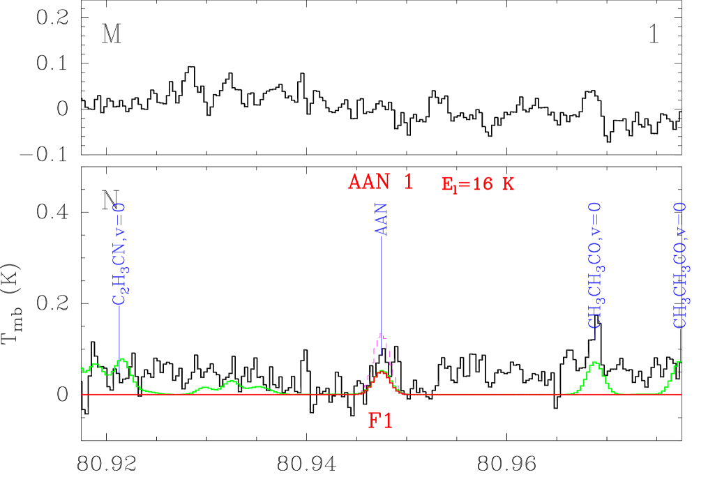
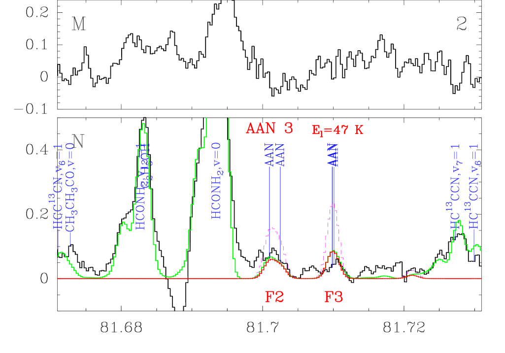
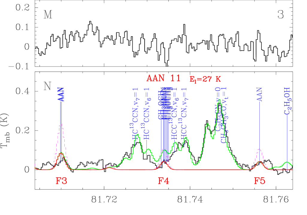
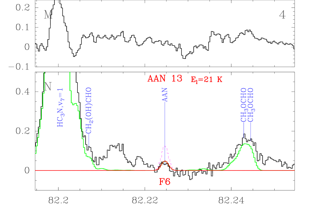
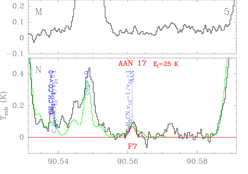
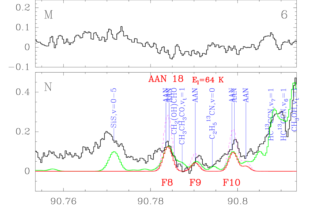
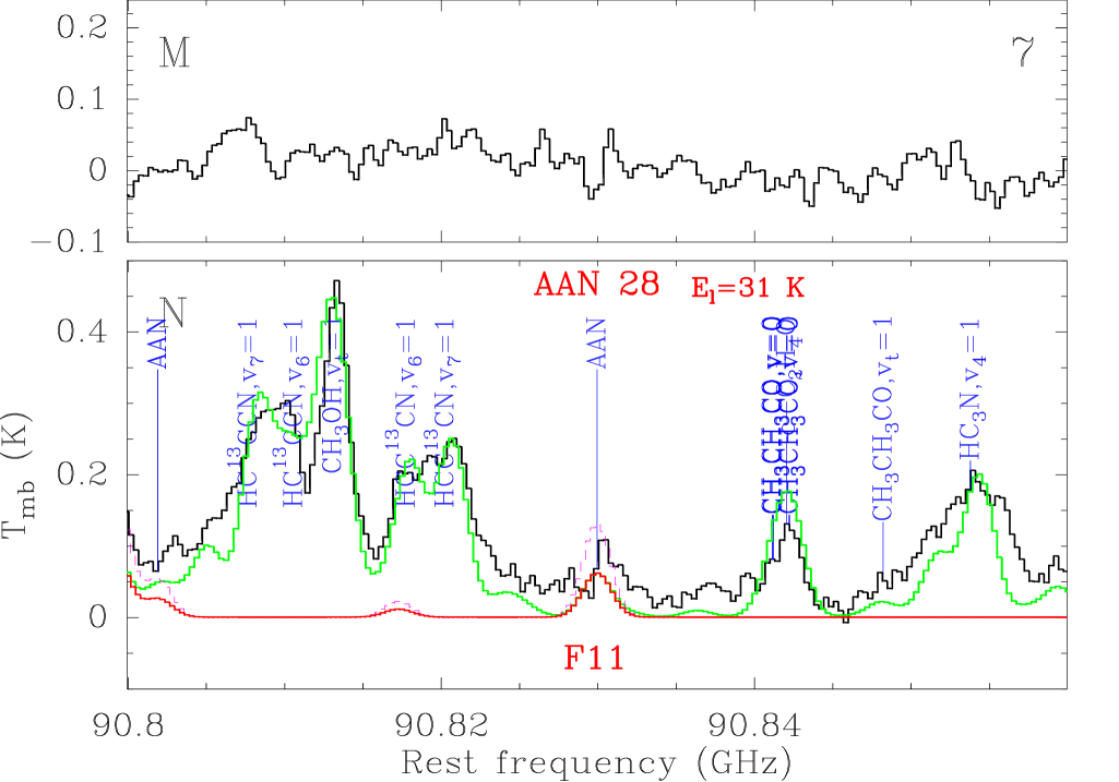
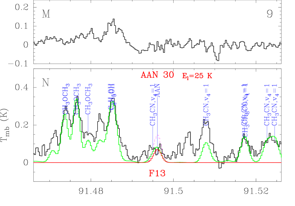
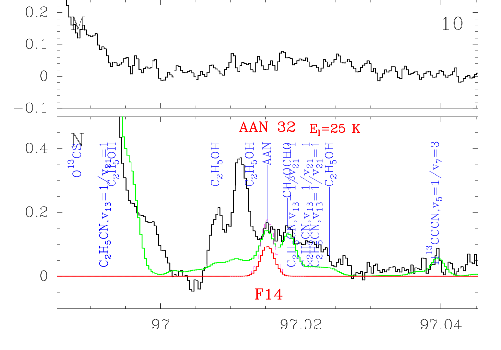
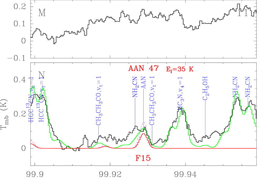
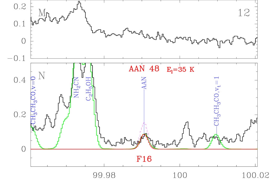
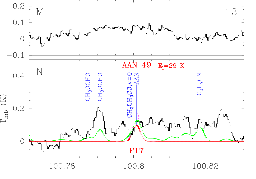
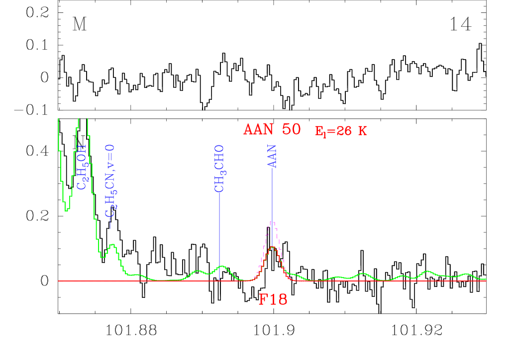
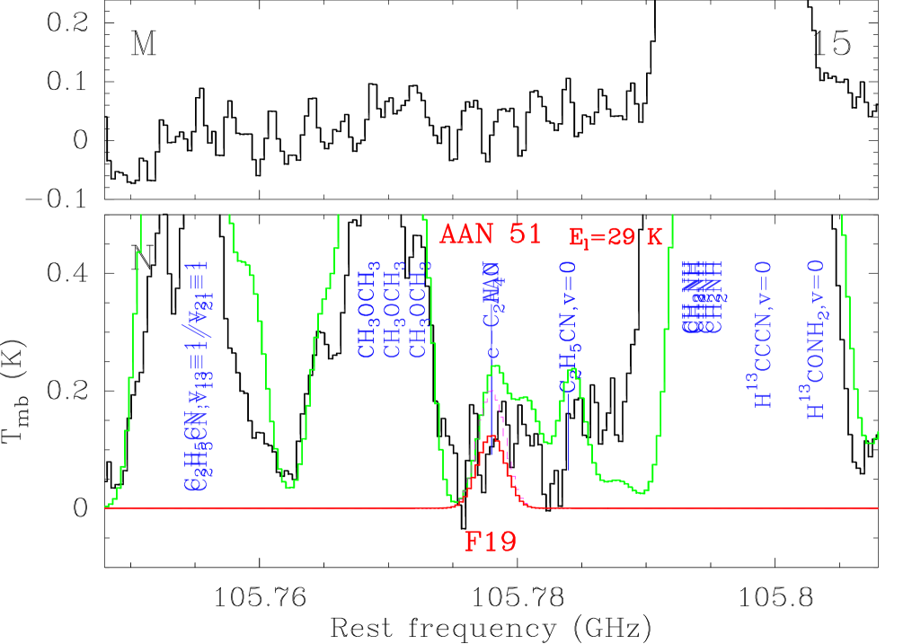
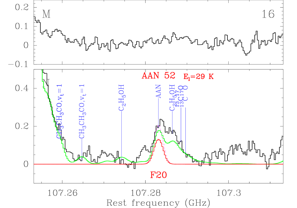
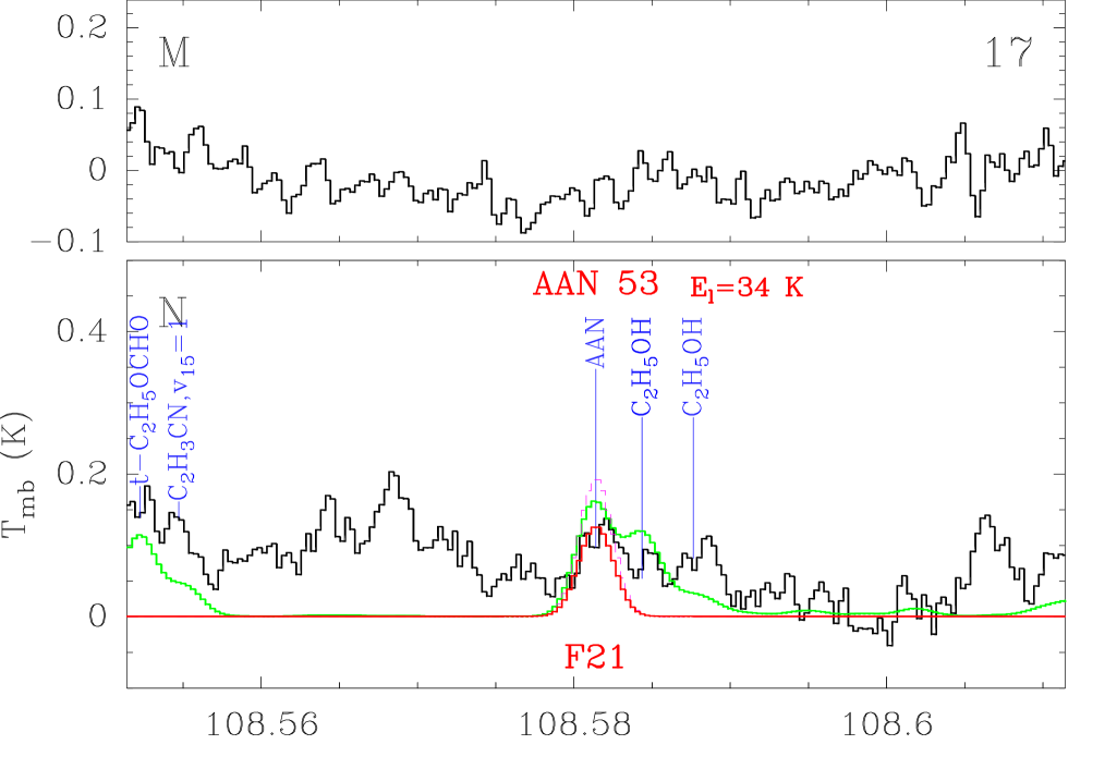
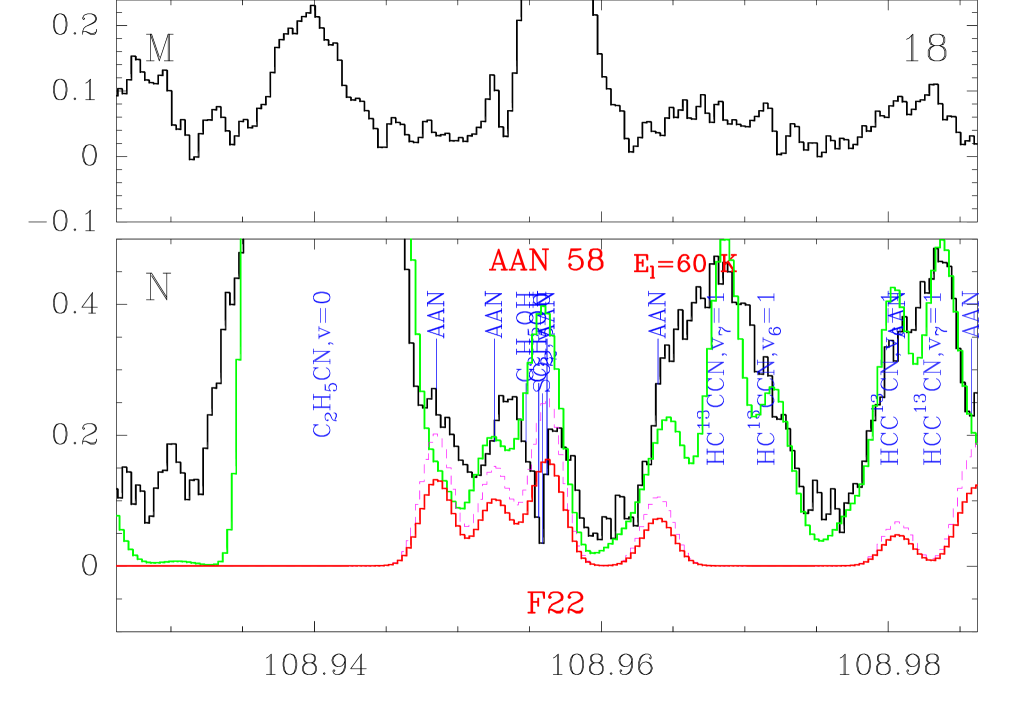
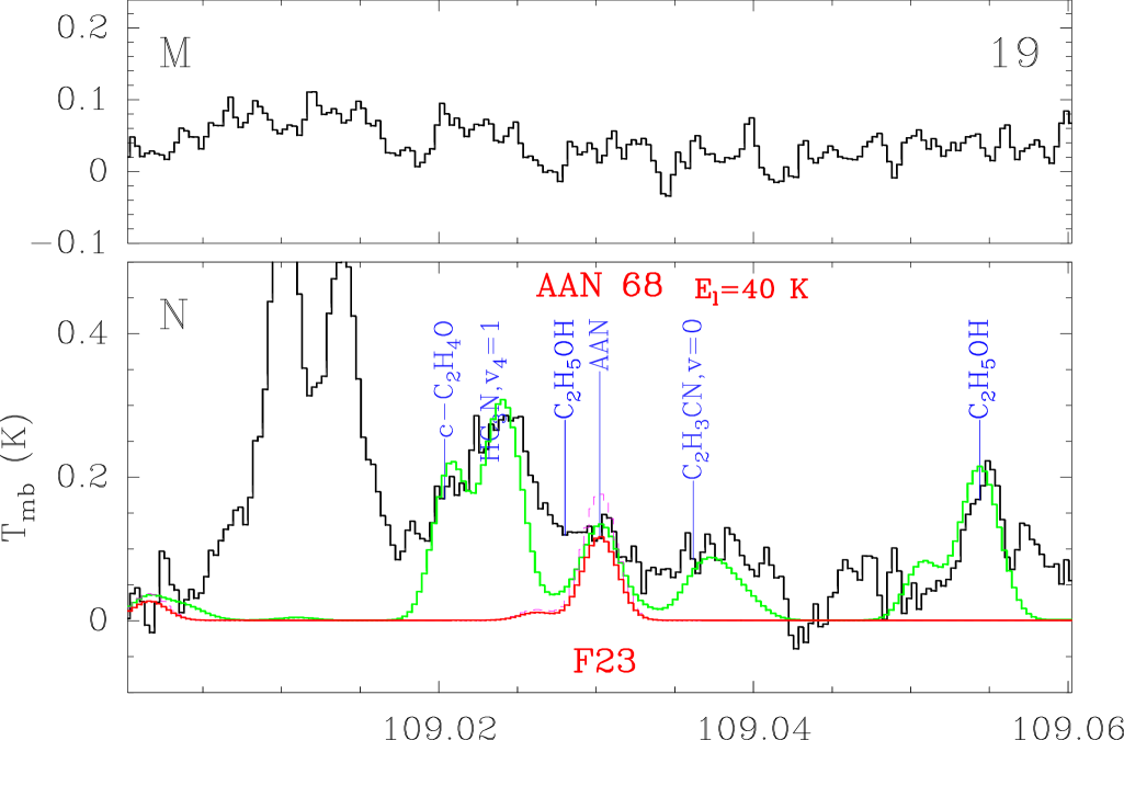
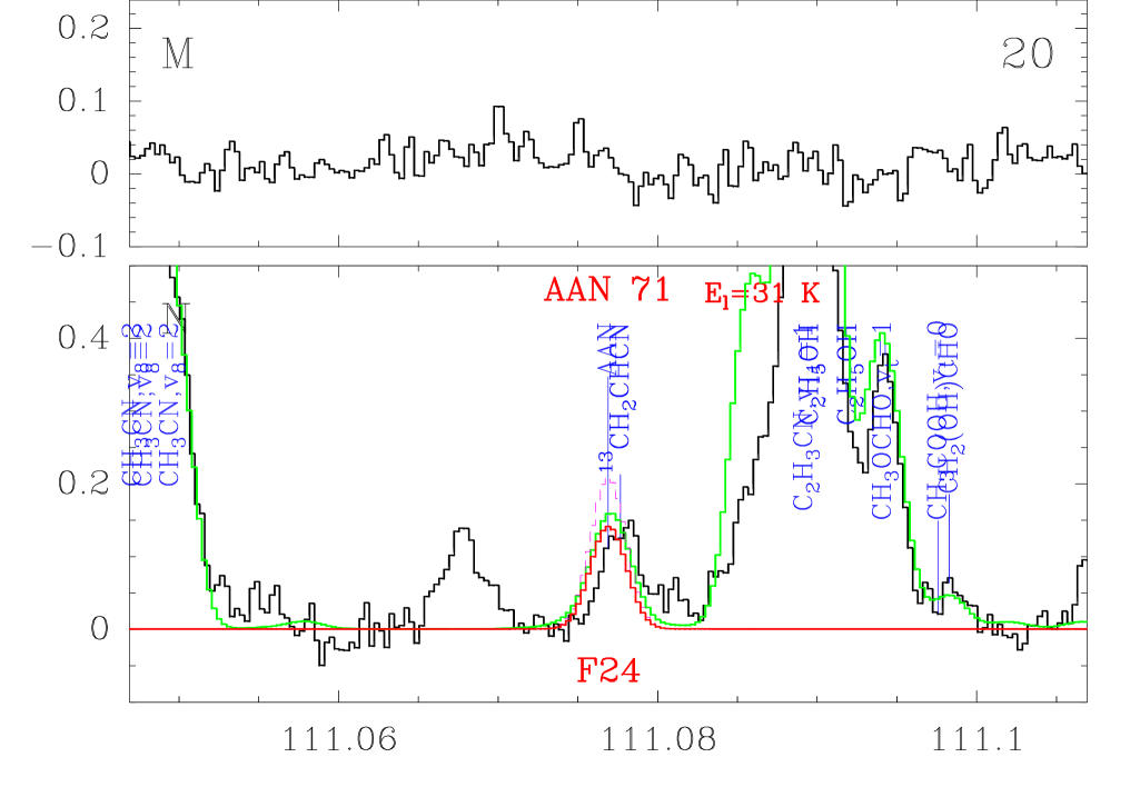
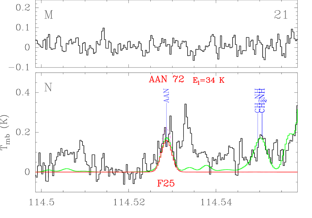
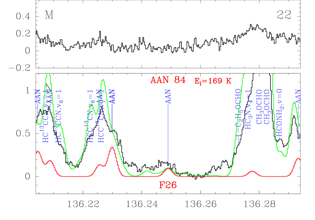
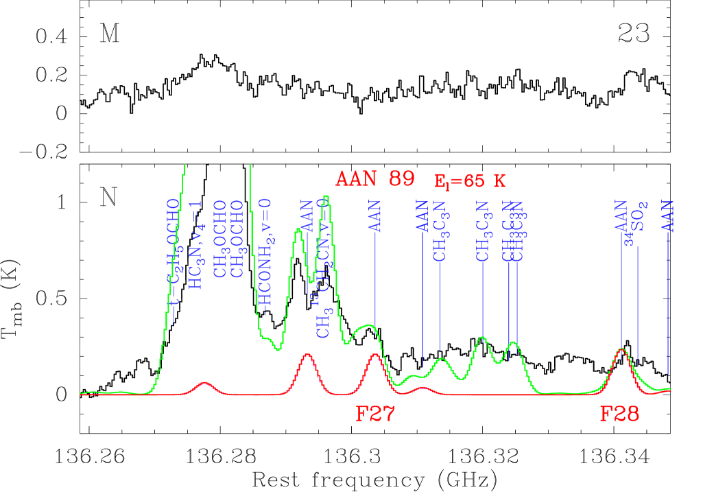
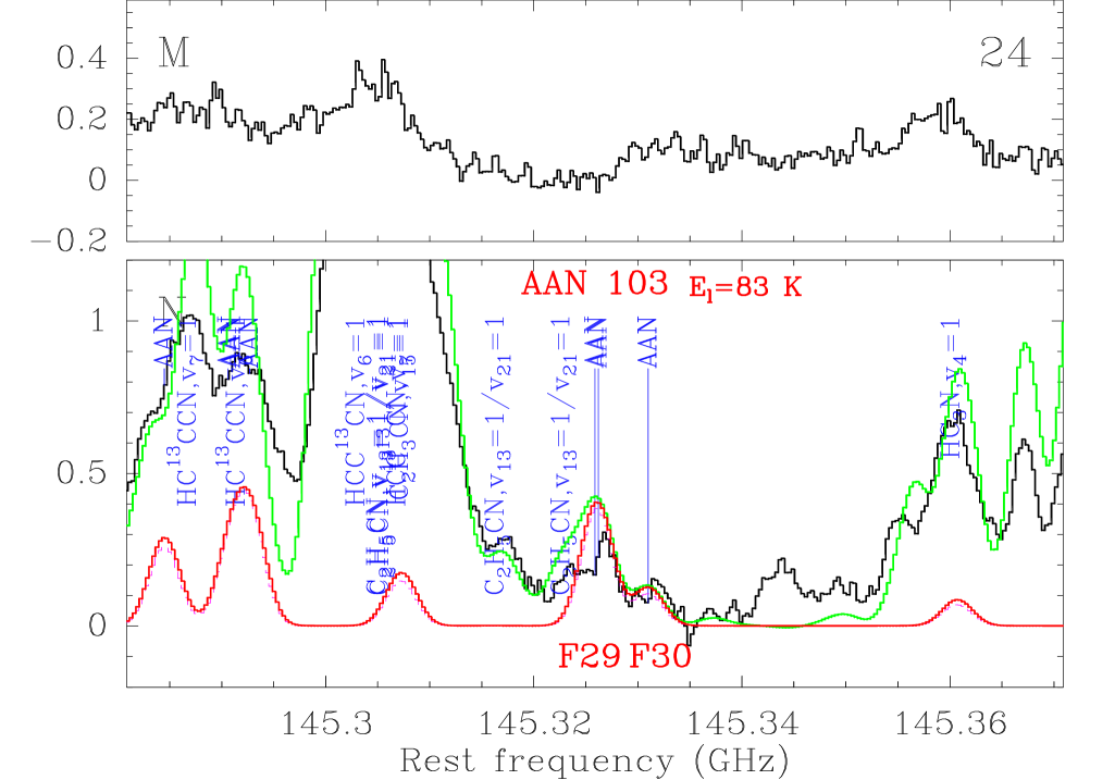
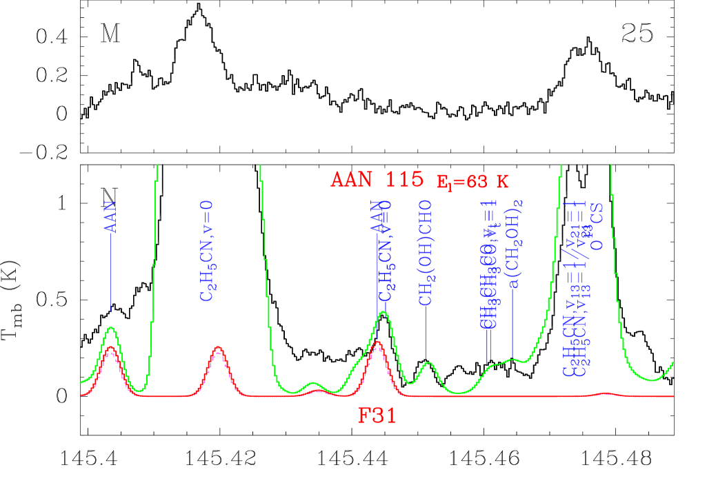
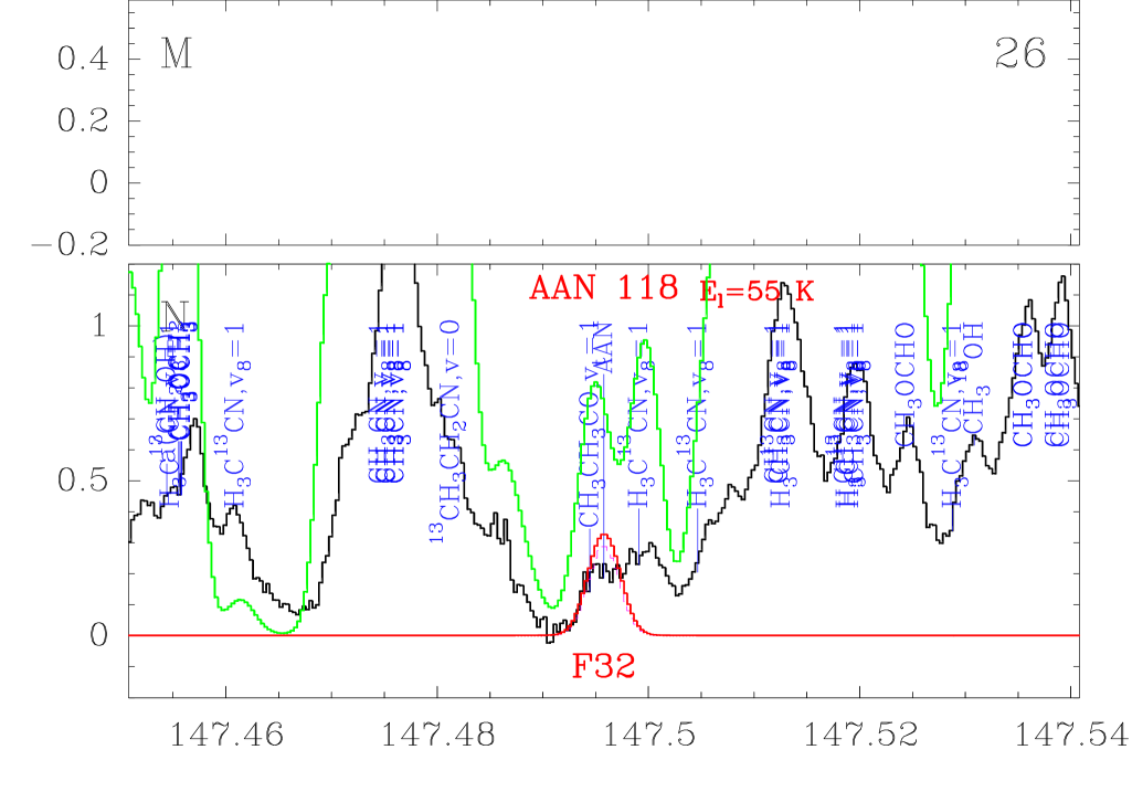
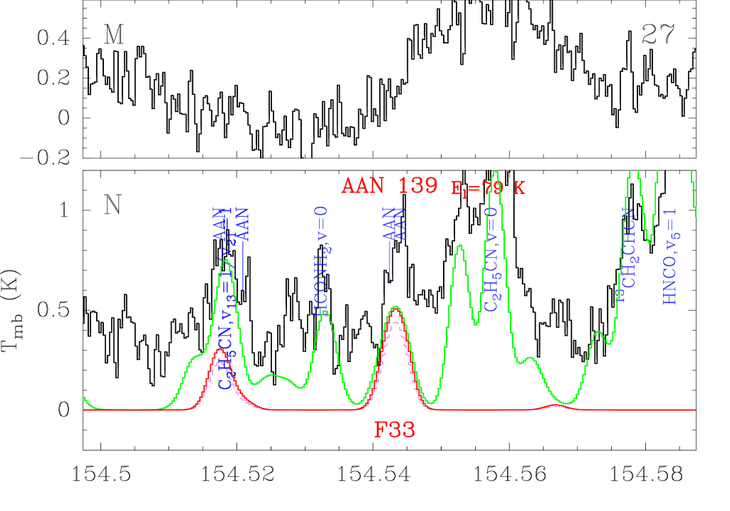
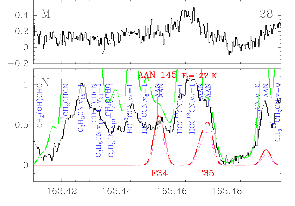
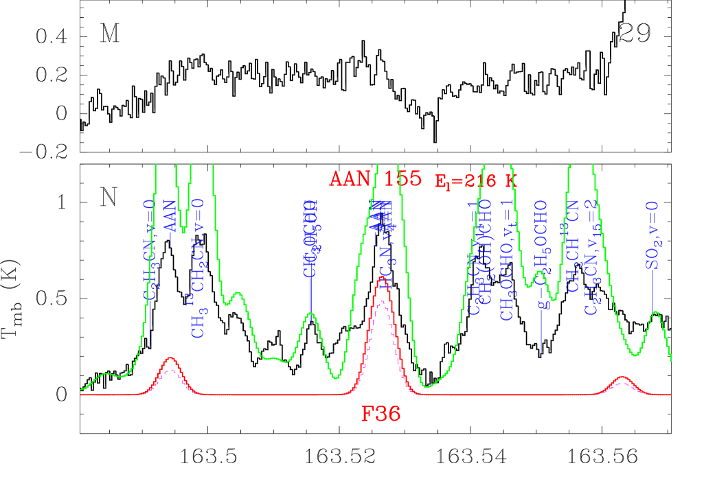
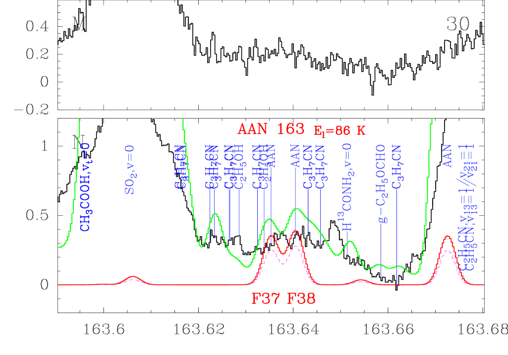
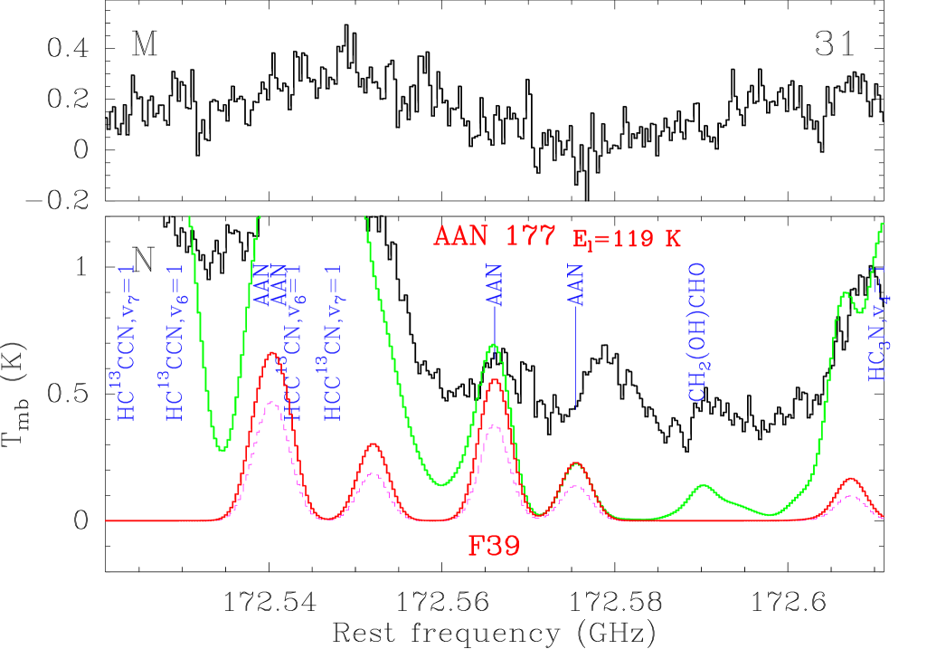
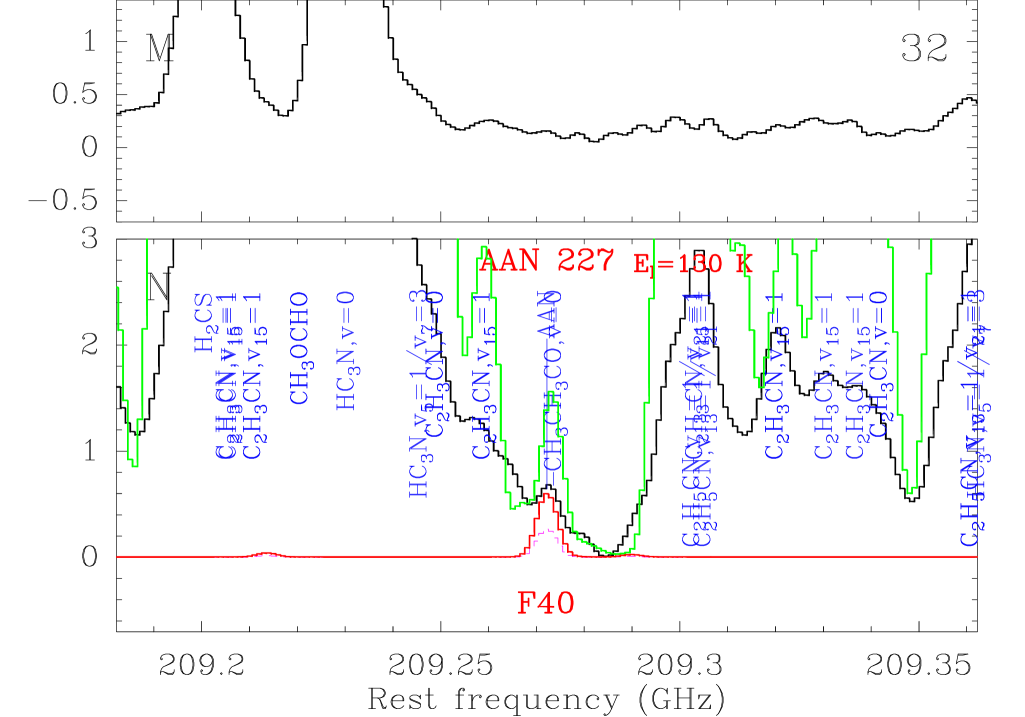
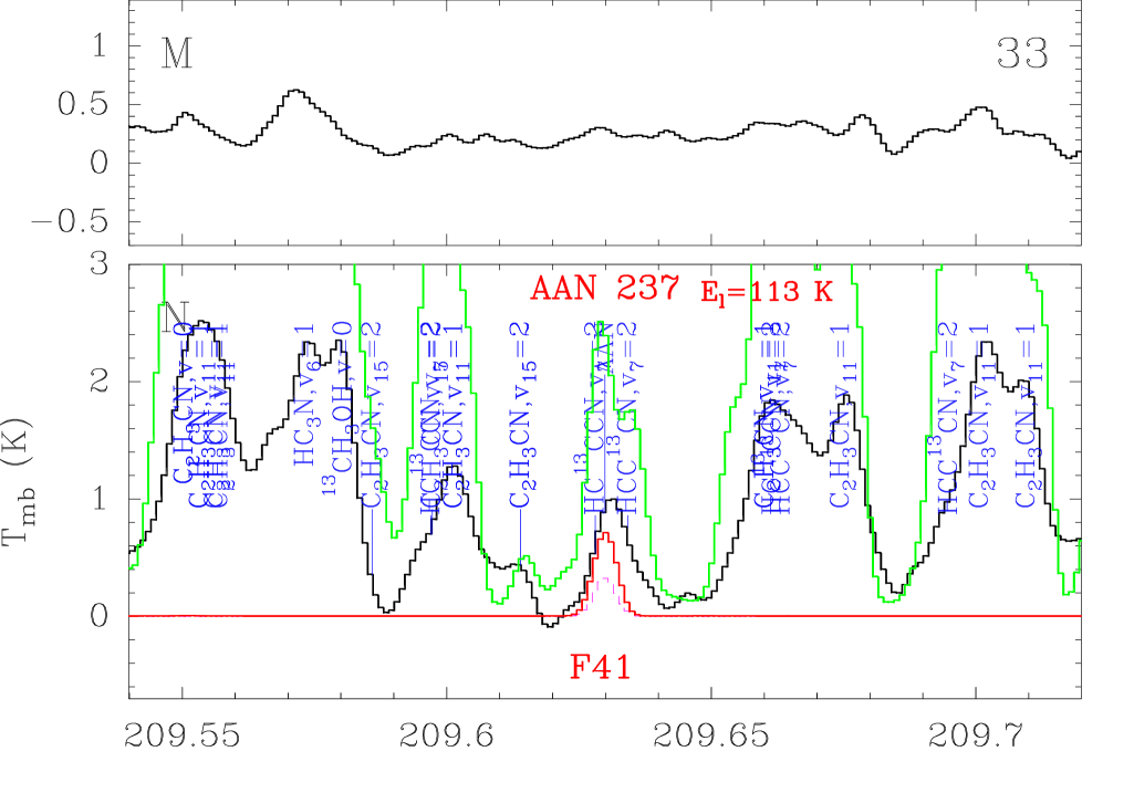
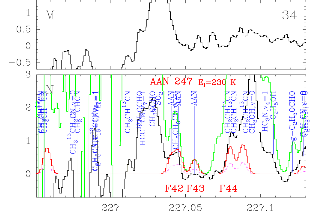
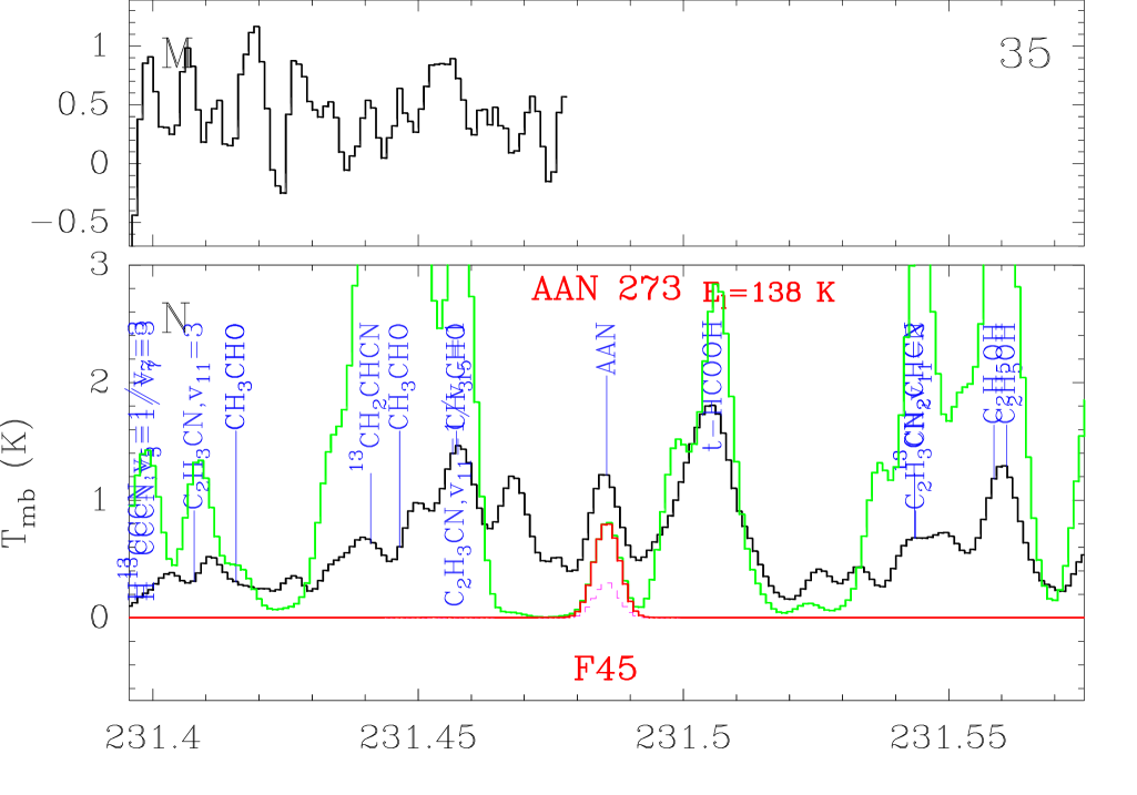
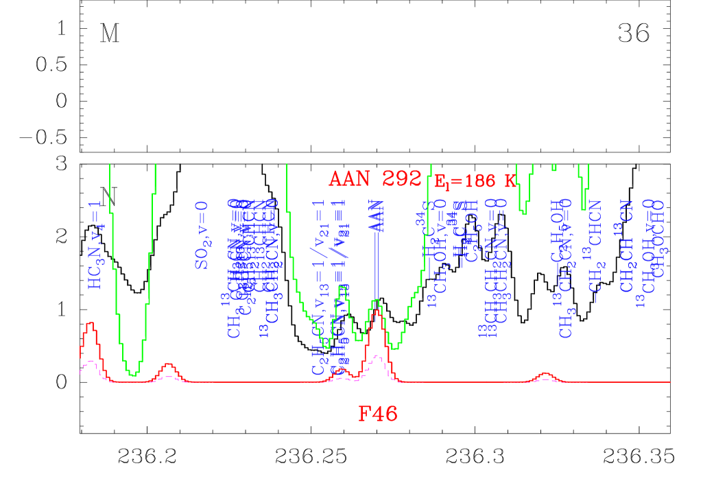
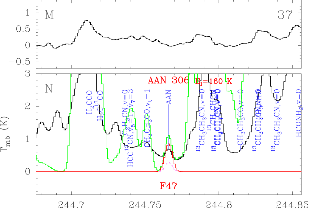
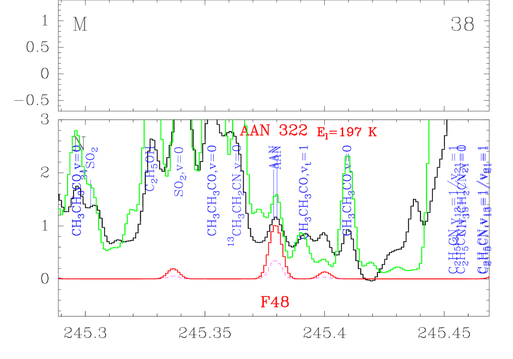
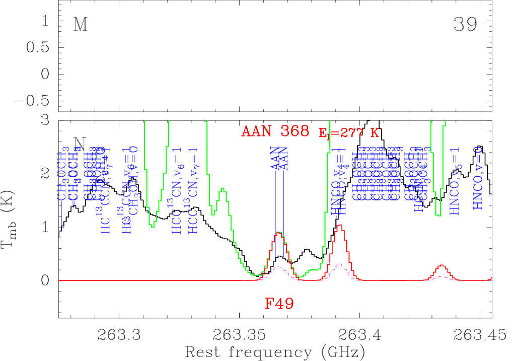
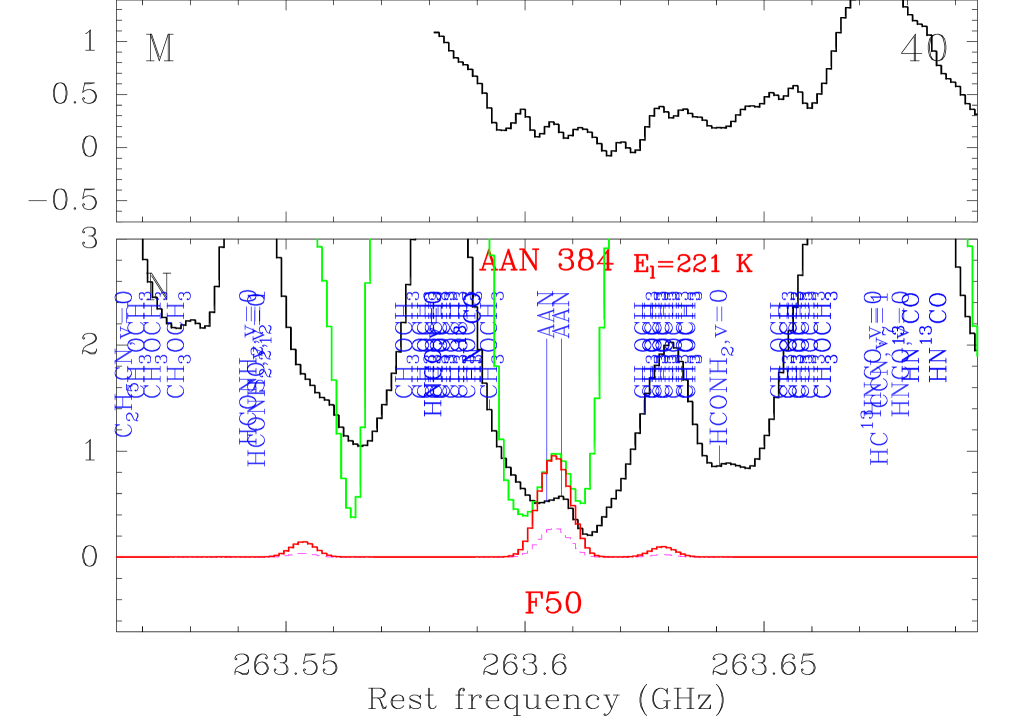
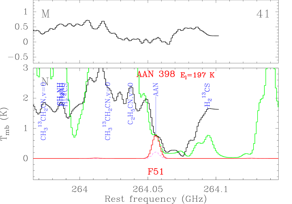
We list in Col. 8 of Table 3 comments about the blends affecting the amino acetonitrile transitions. As can be seen in this table, most of the amino acetonitrile lines covered by our survey of Sgr B2(N) are heavily blended with lines of other molecules and therefore cannot be identified in this source. Only 88 of the 398 transitions are relatively free of contamination from other molecules, known or still unidentified according to our modeling. They are marked “Detected” or “Group detected” in Col. 8 of Table 3, and are listed with more information in Table 4. They correspond to 51 observed features which are shown in Fig. 2 (online material) and labeled in Col. 8 of Table 4. For reference, we show the spectrum observed toward Sgr B2(M) in this figure also. We identified the amino acetonitrile lines and the blends affecting them with the LTE model of this molecule and the LTE model including all molecules (see Sect. 3.2). The parameters of our best-fit LTE model of amino acetonitrile are listed in Table 5, and the model is overlaid in red on the spectrum observed toward Sgr B2(N) in Fig. 2. The best-fit LTE model including all molecules is shown in green in the same figure. The source size we used to model the amino acetonitrile emission was derived from our interferometric measurements (see Sect. 3.4 below).
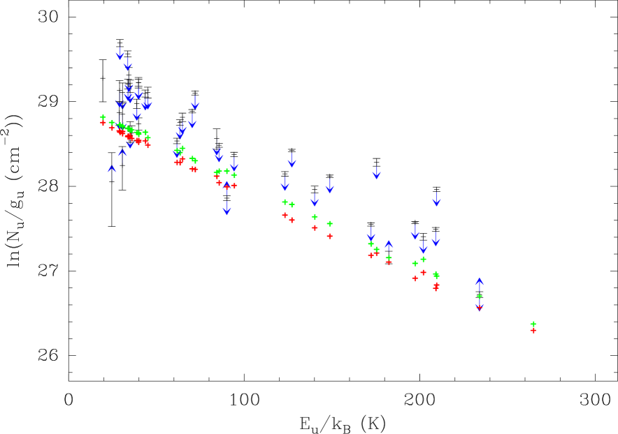
For the frequency range corresponding to each observed amino acetonitrile feature, we list in Table 4 the integrated intensities of the observed spectrum (Col. 10), of the best-fit model of amino acetonitrile (Col. 11), and of the best-fit model including all molecules (Col. 12). In these columns, the dash symbol indicates transitions belonging to the same feature. Columns 1 to 7 are the same as in Table 3. The uncertainty given in Col. 10 was computed using the estimated noise level of Col. 7. These measurements are plotted in the form of a population diagram in Fig. 3, which plots upper level column density divided by statistical weight, , versus the upper level energy in Kelvins (see Goldsmith & Langer 1999). The data are shown in black and our best-fit model of amino acetonitrile in red. Out of 21 features encompassing several transitions, 10 contain transitions with different energy levels and were ignored in the population diagram (features 2, 3, 8, 33, 34, 35, 36, 42, and 49). We used equation A5 of Snyder et al. (2005) to compute the ordinate values. This equation assumes optically thin emission. To estimate by how much line opacities affect this diagram, we applied the opacity correction factor (see Goldsmith & Langer 1999; Snyder et al. 2005) to the modeled intensities, using the opacities from our radiative transfer calculations (Col. 9 of Table 4); the result is shown in green in Fig. 3. The population diagram derived from the modeled spectrum is slightly shifted upwards but its shape, in particular its slope (the inverse of which approximately determines the rotation temperature), is not significantly changed, since does not vary much (from 0.04 to 0.24). The populations derived from the observed spectrum in the optically thin approximation are therefore not significantly affected by the optical depth of the amino acetonitrile transitions333Note that our modeled spectrum is anyway calculated with the full LTE radiative transfer which takes into account the optical depth effects (see Sect. 3.2).. The scatter of the black crosses in Fig. 3 is therefore dominated by the blends with other molecules and uncertainties in the baseline removal (indicated by the downwards and upwards blue arrows, respectively). From this analysis, we conclude that our best-fit model for amino acetonitrile is fully consistent with our 30m data of Sgr B2(N).
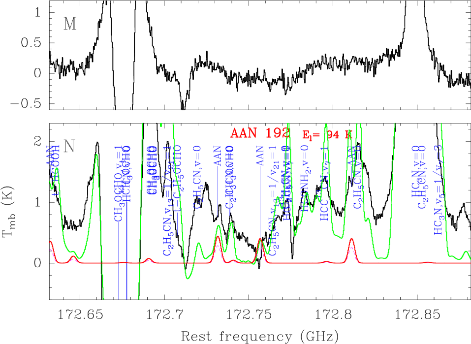
Finally, as mentioned above, the 310 transitions of Table 3 not shown in Fig. 2 are all but one heavily blended with transitions of other molecules and cannot be clearly identified in Sgr B2(N). The single exception is amino acetonitrile transition 192 shown in Fig. 4. There are too many blended lines in this frequency range to properly remove the baseline. It is very uncertain and the true baseline is most likely at a lower level than computed here. The presence of several H13CN 21 velocity components in absorption also complicates the analysis. Therefore it is very likely that the (single) apparent disagreement concerning transition 192 between our best-fit model and the 30m spectrum observed toward Sgr B2(N) is not real and does not invalidate our claim of detection of amino acetonitrile.
3.4 Mapping amino acetonitrile with the PdBI
The two 3 mm spectral windows of the PdBI were chosen to cover the five amino acetonitrile features F2 to F6. The spectra toward Sgr B2(N) are shown for both windows toward 3 positions P1, P2, and P3 in Fig. 5a to f. Many lines are detected, the strongest one being a line from within the vibrationally excited state v7=1 of cyanoacetylene (HC3N) at 82.2 GHz. We also easily detect lines from within its vibrationally excited state v4=1, from its isotopologues HC13CCN and HCC13CN in the v7=1 state, from ethyl cyanide (C2H5CN), as well as two unidentified lines at 82.213 and 82.262 GHz. At a lower level, we find emission for all the amino acetonitrile features F2 to F6, and we also detect methylformate (CH3OCHO).
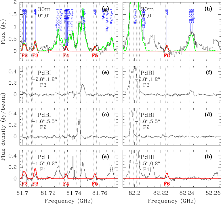
The integrated intensity maps of the amino acetonitrile features F2 to F6 are presented in Fig. 6a to e, along with two maps of ethyl cyanide (Fig. 6g and h), four maps of cyanoacetylene in the vibrationally excited states v4=1 and v7=1 (Fig. 6j to m), one map of its isotopologue HC13CCN in the state v7=1 (Fig. 6i), one map of methylformate (Fig. 6n), and a reference map computed on the PdBI line-free frequency range between F2 and F3 (Fig. 6f). The frequency intervals used to compute the integrated intensities are given in Col. 3 and 4 of Table 6 and shown with dotted lines in Fig. 5. We used the fitting routine GAUSS2D of the GILDAS software to measure the position, size, and peak flux of each integrated emission. The results are listed in Col. 6 to 11 in Table 6. We label P1 the mean peak position of features F2 to F6, P2 the northern peak position of ethyl cyanide, and P3 the peak position of methylformate (see Table 7 and the plus symbols in Fig. 6). Finally, the PdBI velocity-integrated flux spatially integrated over the emitting region is listed in Col. 12 and the 30m velocity-integrated intensity is given in Col. 13.
| Molecule | Fa | fminb | fmaxb | Fpeakd | d | d | d | d | P.A.d | |||
| (MHz)) | (MHz) | (Jy/beam km/s) | (′′) | (′′) | (′′) | (′′) | (∘) | (Jy km/s) | (Jy km/s) | |||
| (1) | (2) | (3) | (4) | (5) | (6) | (7) | (8) | (9) | (10) | (11) | (12) | (13) |
| AAN | F2 | 81700.21 | 81703.33 | 0.09 | 0.68 | -1.60 0.05 | 0.30 0.22 | 3.9 0.4 | 2.00 0.10 | 20.5 0.1 | 1.76 | 2.89 |
| AAN | F3 | 81708.02 | 81712.08 | 0.10 | 0.68 | -1.25 0.06 | 0.02 0.24 | 3.8 0.5 | 1.39 0.12 | 10.1 0.0 | 1.24 | 1.75 |
| AAN | F4 | 81732.71 | 81734.90 | 0.06 | 0.44 | -1.70 0.06 | 0.35 0.24 | 3.6 0.5 | 1.54 0.12 | 14.0 0.0 | 0.86 | 0.98 |
| AAN | F5 | 81754.90 | 81757.40 | 0.06 | 0.24 | -1.52 0.10 | 0.03 0.44 | 3.2 0.9 | 1.20 0.21 | 12.5 1.1 | 0.30 | 1.15 |
| AAN | F6 | 82223.46 | 82226.27 | 0.06 | 0.43 | -1.43 0.06 | 0.28 0.24 | 3.5 0.5 | 1.54 0.11 | 6.0 0.4 | 0.79 | 0.97 |
| Reference | 81704.27 | 81707.08 | 0.07 | … | … | … | … | … | … | … | … | |
| C2H5CN | HV | 81741.77 | 81744.90 | 0.11 | 2.05 | -1.64 0.02 | 5.58 0.09 | 3.8 0.2 | 1.50 0.04 | 5.7 0.0 | 4.07 | 6.38 |
| C2H5CN | LV | 81745.21 | 81749.27 | 0.15 | 2.82 | -1.74 0.02 | 0.46 0.09 | 3.8 0.2 | 2.87 0.04 | 13.7 0.0 | 10.43 | 12.94 |
| HC13CCN v7=1 | 81726.15 | 81728.96 | 0.09 | 2.20 | -1.35 0.02 | 0.60 0.07 | 3.7 0.1 | 1.68 0.03 | 12.6 0.0 | 4.98 | 4.81 | |
| HC3N v4=1 | 81767.71 | 81771.15 | 0.10 | 2.14 | -1.43 0.02 | 0.28 0.08 | 3.6 0.2 | 1.35 0.04 | 9.9 0.0 | 3.78 | 3.85 | |
| HC3N v7=1g | HV | 82196.27 | 82198.77 | 0.25 | 6.17 | -2.16 0.02 | 0.69 0.07 | 4.0 0.1 | 1.84 0.03 | 16.2 22.5 | 16.05 | 23.88 |
| 3.36 | -1.50 0.03 | 5.25 0.12 | 4.0 0.2 | 1.36 0.06 | 5.5 22.5 | 5.35 | … | |||||
| HC3N v7=1 | LV | 82199.40 | 82201.58 | 0.36 | 9.06 | -1.67 0.02 | 0.42 0.07 | 3.7 0.1 | 2.50 0.03 | 10.2 22.5 | 31.04 | 33.48 |
| HC3N v7=1 | BW | 82202.52 | 82203.77 | 0.12 | 3.37 | -0.71 0.01 | 0.24 0.06 | 3.1 0.1 | 2.77 0.03 | 45.0 0.0 | 11.75 | 12.39 |
| CH3OCHO | 82242.21 | 82245.33 | 0.10 | 0.67 | -2.83 0.06 | 1.23 0.26 | 4.8 0.5 | 2.58 0.12 | 9.5 22.5 | 2.83 | 6.62 | |
-
Feature numbered like in Col. 8 of Table 4 for amino acetonitrile (AAN). HV and LV mean ”high” and ”low” velocity components, respectively, and BW means blueshifted linewing.
-
Frequency range over which the intensity was integrated.
-
Noise level in the integrated intensity map shown in Fig. 6.
-
Peak flux, offsets in right ascension and declination with respect to the reference position of Fig. 6, major and minor diameters (FWHM), and position angle (East from North) derived by fitting an elliptical 2D Gaussian to the integrated intensity map shown in Fig. 6. The uncertainty in Col. 11 is the formal uncertainty given by the fitting routine GAUSS2D, while the uncertainties correspond to the beam size divided by two times the signal-to-noise ratio in Col. 7 and 8 and by the signal-to-noise ratio in Col. 9 and 10.
-
Flux spatially integrated over the region showing emission in the integrated intensity map of Fig. 6.
-
Integrated flux of the 30m spectrum computed over the frequency range given in Col. 3 and 4.
-
The two emission peaks of Fig. 6k were fitted separately.
We present in Fig. 6o the map of continuum emission at 82.0 GHz, integrated over line-free frequency ranges. The continuum emission has a complex structure. The main region peaks at , , i.e. within 0.1 of the position of the ultracompact Hii region K2. It also shows hints of emission at the position of the ultracompact Hii regions K1 and K3, although the spatial resolution is too poor to resolve them (see, e.g., Gaume et al. 1995). There are other secondary peaks. One of them coincides with the peak of the shell-like Hii region K6 while another one is located close () to the peak of the shell-like Hii region K5 and traces most likely the same shell. On the other hand, we detect no 3.7 mm emission at the position of the weak ultracompact Hii region K9.69 (Gaume et al. 1995).
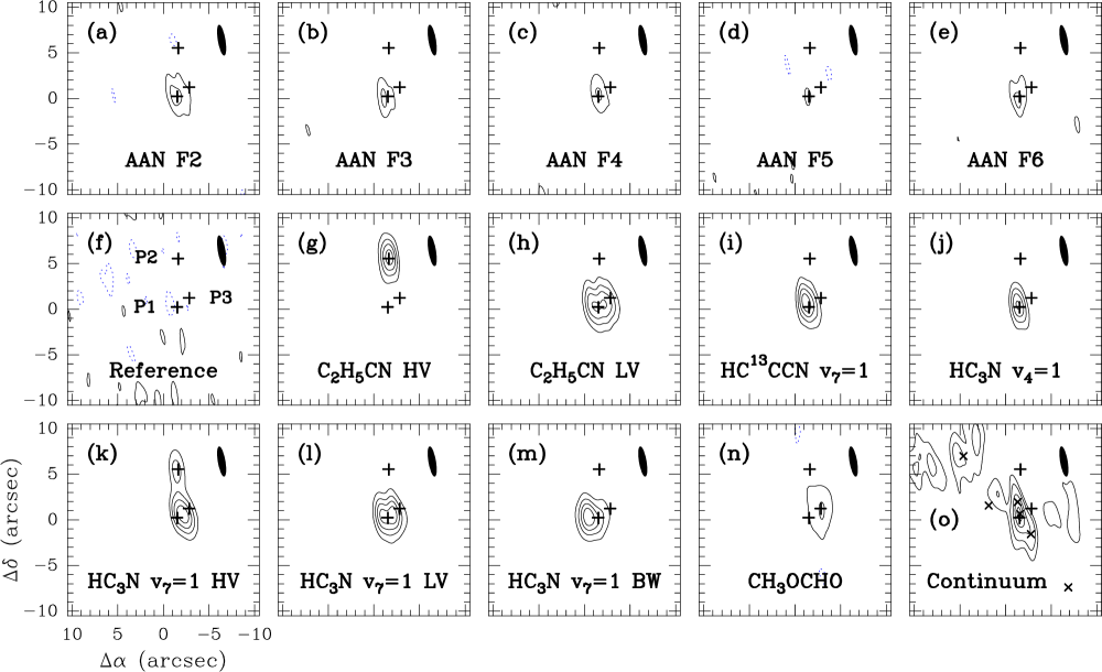
The strong lines detected with the PdBI (Fig. 6g to n) allow us to gain insight into the distribution of molecular line emission in Sgr B2(N). The double-peaked profile of ethyl cyanide seen with the 30m telescope (see Fig. 5g) is resolved with the PdBI into two sources P1 and P2 separated by about 5.3 (see Fig. 5a, c, Fig. 6g, h, and Table 7). P1 and P2 are spatially and kinematically coincident with the quasi-thermal methanol emission cores “i” and “h” within and , respectively (Mehringer & Menten 1997). Cores “i” and “h” were both previously detected in ethyl cyanide (Liu & Snyder 1999; Hollis et al. 2003; Jones et al. 2007). Many molecules (but not amino acetonitrile within the limits of our sensitivity) actually show this double-peaked profile in our 30m survey of Sgr B2(N) and are most likely emitted by these two sources. P1 and P2 are also detected in our PdBI data in the vibrationally excited state v7=1 of cyanoacetylene (see Fig. 5b, d, and Fig. 6k, l), and there is a hint of emission toward P2 in the isotopologue HC13CCN while P1 is easily detected (see Fig. 5c and a). In addition, the wings of the main component of cyanoacetylene v7=1 are spatially shifted: the redshifted wing peaks about North-West of P1 while the blueshifted wing peaks about East of P1 (Fig. 6k and m). This East-West velocity gradient was previously reported by several authors (e.g. Lis et al. 1993; de Vicente et al. 2000; Hollis et al. 2003). Although it could result from cloud rotation, it is most likely a sign of outflow activity (see, e.g., Liu & Snyder 1999). The transition with highest energy in our PdBI sample is a transition of cyanoacetylene in the vibrationally excited state v4=1 ( K). Within the limits of our sensitivity, we detect emission only toward P1 in this highly excited transition (Fig. 6j). Finally, methylformate peaks at a position significantly offset from P1, at to the North-West (Fig. 6n). It has no counterpart in the continuum map of Fig. 6o. To sum up, our PdBI data reveal three main positions of molecular line emission (P1 and P2 corresponding to the methanol cores “i” and “h”, and P3 the peak position of methylformate), and an East-West velocity gradient around P1.
Within the limits of our sensitivity, the amino acetonitrile features F2 to F6 detected with the PdBI show only one peak, and they all peak at the same position (Fig. 6a to e). We are confident that the emission detected in features F2 to F6 is not contaminated by the continuum since no significant signal is detected in the reference map (Fig. 6f). Their weighted-mean peak position was labeled P1 above (offset , , see Table 7). The fact that all features are detected at the same position is consistent with their assignment to the same molecule (see above the shifted position of methylformate for instance). The deconvolved major and minor axes of the emission detected in features F2 to F6 are in the range 0–2.2 and 1.0–1.9, respectively. The amino acetonitrile emission is therefore slightly resolved and has a size of roughly 2 FWHM, which we used for the LTE modeling. The spatially integrated fluxes of F4 and F6 agree within 20 with the fluxes measured with the 30m telescope (see Col. 12 and 13 of Table 6). The emission detected with the 30m telescope in these two features of amino acetonitrile is therefore compact (2) and was not filtered out by the interferometer. The other features F2, F3, and F5 have 30m fluxes 1.6, 1.4, and 3.8 times larger than the PdBI fluxes, respectively: the emission filtered out by the interferometer most likely corresponds to the unidentified transitions blended with these amino acetonitrile features (see Fig. 5a). In addition, the low signal-to-noise ratio of feature F5 detected with the PdBI may significantly affect the flux measurement.
We used the parameters of the 30m model (see Table 5) to compute a model spectrum of amino acetonitrile with the spatial resolution of the PdBI (using the geometrical mean of the elliptical beam). The agreement with the peak spectrum is good, within a factor of 2 (see Fig. 5a and b). The small discrepancy may come from the somewhat uncertain source size and from our approximate modeling of the interferometric beam pattern: spherical beam and full uv coverage for the model versus elliptical beam and partially sampled uv coverage for the observations. Overall, our LTE model of amino acetonitrile is therefore well consistent with the compact emission detected with the PdBI.
3.5 Mapping amino acetonitrile with the ATCA
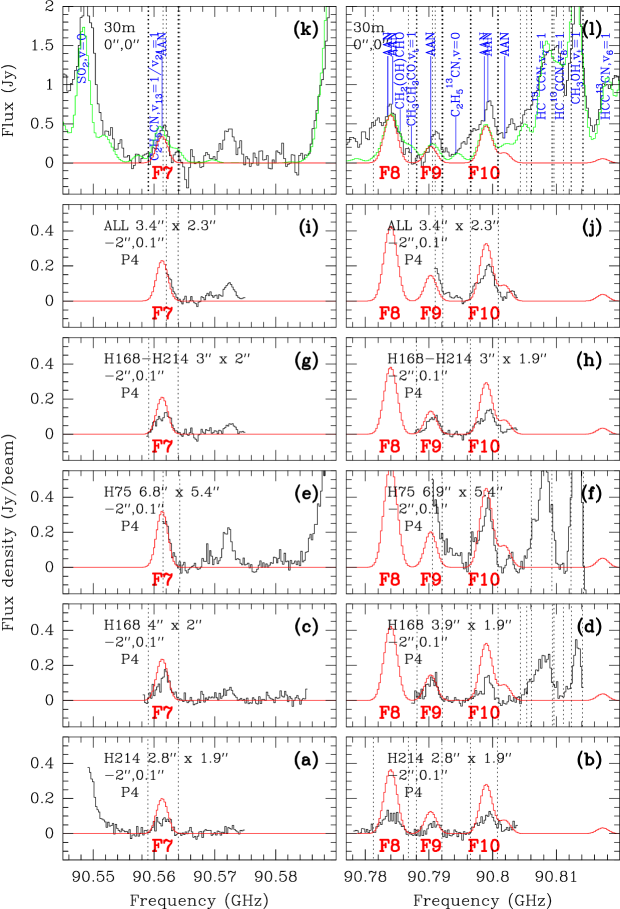
The two 3mm spectral windows of the ATCA were chosen to cover the four amino acetonitrile features F7 to F10. The spectra toward position P4 of Sgr B2(N) (offset ,0.1) are presented for both windows in Fig. 7. Since the spectral windows were not exactly the same in each configuration (see Sect. 2.3), we show the spectra for each configuration (Fig. 7a to f), plus the combination of the two broadest ones (Fig. 7g and h), and the combination of all three configurations (Fig. 7i and j). Nearly all the lines seen with the 30m telescope are detected with the ATCA toward P4. In the 90.6 GHz band, we detect the blue wing of an SO2 transition (Fig. 7a), the red wing of an HC13CCN ground-state transition (Fig. 7e), an unidentified line, and feature F7. In the 90.8 GHz band, we detect the low-velocity component of a vt=1 transition of methanol, the low-velocity component of a v7=1 transition of HC13CCN (Fig. 7d and f), and the three amino acetonitrile features F8, F9, and F10. Toward the northern position P5, we detect a second velocity component of methanol vt=1 and HC13CCN v7=1 (not shown in Fig. 7, see below).
| RA (J2000) | Dec (J2000) | Comments | |
| PdBI | |||
| 82 | continuum 82.0 GHz | ||
| P1 | mean AANa F2 to F6 | ||
| P2 | mean HC3N v7=1, C2H5CN | ||
| P3 | peak CH3OCHO | ||
| ATCA | |||
| 95 | mean continuum | ||
| 93.2 and 97.4 GHz | |||
| P4 | mean AAN F7 to F10 | ||
| P5 | mean HC13CCN v7=1, | ||
| CH3OH vt=1 | |||
-
AAN stands for amino acetonitrile.
The integrated intensity maps of the amino acetonitrile features F7 to F10 in the different configurations are presented in Fig. 8a to p, along with maps of the excited states of methanol and HC13CCN (Fig. 8q to v). The frequency intervals used to compute the integrated intensities are given in Col. 3 and 4 of Table 8 and drawn in dotted lines in Fig. 7. We used the fitting routine GAUSS2D of the GILDAS software to measure the position, size, and peak flux of each integrated emission. The results are listed in Col. 6 to 11 of Table 8. We label P4 the weighted-mean peak position of features F7 to F10, computed using the combined configuration H 214 + H 168 (only H 214 for F8), and P5 the average northern peak position of methanol and HC13CCN. The mean peak position P4 is at the offset (, ), and the average position P5 is at (, ) (see coordinates in Table 7 and positions in Fig. 8x). Finally, the ATCA velocity-integrated flux spatially integrated over the emitting region is listed in Col. 12 of Table 8 and the 30m velocity-integrated intensity is given in Col. 13.
| Moleculea | Conf.b | fminc | fmaxc | Fpeake | e | e | e | e | P.A.e | |||
| (MHz)) | (MHz) | (Jy/beam km/s) | (′′) | (′′) | (′′) | (′′) | (∘) | (Jy km/s) | (Jy km/s) | |||
| (1) | (2) | (3) | (4) | (5) | (6) | (7) | (8) | (9) | (10) | (11) | (12) | (13) |
| AAN F7 | E | 90558.99 | 90563.99 | 0.12 | 0.87 | -2.32 0.20 | -0.22 0.13 | 2.9 0.4 | 2.2 0.3 | 29.2 0.1 | 1.12 | 3.06 |
| AAN F7 | I | 90559.05 | 90564.05 | 0.15 | 1.47 | -1.94 0.20 | 0.58 0.10 | 3.6 0.4 | 2.7 0.2 | -79.8 1.5 | 1.73 | 3.06 |
| AAN F7 | C | 90561.48 | 90564.23 | 0.10 | 1.53 | -0.96 0.21 | 0.71 0.17 | 7.0 0.4 | 4.8 0.3 | -80.3 0.0 | 1.37 | 1.79 |
| AAN F7 | M | 90559.13 | 90563.96 | 0.12 | 1.19 | -2.10 0.16 | 0.25 0.10 | 3.1 0.3 | 2.7 0.2 | 83.5 0.0 | 1.71 | 2.96 |
| AAN F7 | A | 90562.03 | 90563.96 | 0.06 | 0.61 | -1.23 0.15 | 0.26 0.10 | 5.3 0.3 | 3.3 0.2 | 87.1 22.5 | 1.37 | 1.00 |
| AAN F8 | E | 90781.27 | 90786.77 | 0.21 | 1.22 | -1.94 0.24 | -0.18 0.16 | 3.8 0.5 | 2.1 0.3 | 45.0 0.0 | 1.70 | 7.23 |
| AAN F9 | E | 90788.02 | 90792.02 | 0.09 | 0.45 | -1.70 0.29 | -0.06 0.19 | 3.4 0.6 | 1.9 0.4 | 45.0 0.1 | 0.49 | 2.14 |
| AAN F9 | I | 90788.11 | 90792.11 | 0.13 | 0.97 | -1.77 0.26 | 0.23 0.13 | 3.6 0.5 | 2.2 0.3 | -84.0 0.0 | 1.01 | 2.14 |
| AAN F9 | C | 90790.54 | 90792.04 | 0.10 | 2.00 | -1.25 0.16 | 0.49 0.13 | 6.1 0.3 | 5.8 0.3 | -45.0 0.0 | 1.86 | 1.59 |
| AAN F9 | M | 90788.04 | 90792.16 | 0.10 | 0.85 | -1.67 0.17 | 0.02 0.11 | 3.1 0.3 | 2.4 0.2 | 75.9 0.1 | 1.07 | 2.14 |
| AAN F9 | A | 90790.95 | 90792.16 | 0.05 | 0.63 | -1.26 0.14 | 0.23 0.09 | 4.8 0.3 | 3.9 0.2 | 84.5 0.0 | 1.51 | 1.31 |
| AAN F10 | E | 90796.52 | 90800.77 | 0.16 | 1.17 | -2.51 0.20 | 0.02 0.13 | 2.7 0.4 | 2.2 0.3 | -81.2 0.2 | 1.38 | 6.48 |
| AAN F10 | I | 90796.61 | 90800.86 | 0.10 | 0.93 | -1.81 0.21 | 0.20 0.11 | 3.3 0.4 | 2.0 0.2 | 82.3 0.0 | 0.79 | 6.19 |
| AAN F10 | C | 90796.54 | 90800.79 | 0.15 | 3.36 | -1.08 0.15 | 0.28 0.12 | 6.6 0.3 | 4.9 0.2 | -77.7 0.0 | 2.78 | 6.48 |
| AAN F10 | M | 90796.52 | 90800.88 | 0.13 | 1.32 | -2.28 0.15 | 0.03 0.09 | 2.9 0.3 | 2.2 0.2 | 83.7 22.5 | 1.42 | 6.48 |
| AAN F10 | A | 90796.52 | 90800.88 | 0.13 | 1.82 | -1.66 0.12 | 0.12 0.08 | 4.5 0.2 | 3.1 0.2 | -89.3 22.5 | 3.24 | 6.48 |
| HC13CCN v7=1 HV | I | 90804.36 | 90805.36 | 0.05 | 0.49 | -1.94 0.20 | 5.16 0.10 | 3.0 0.4 | 2.0 0.2 | 84.4 0.0 | 0.41 | 2.39 |
| HC13CCN v7=1 LV | I | 90806.11 | 90809.36 | 0.14 | 2.74 | -1.56 0.10 | 0.55 0.05 | 3.7 0.2 | 2.1 0.1 | 83.6 0.0 | 2.69 | 10.30 |
| HC13CCN v7=1 LV | C | 90806.04 | 90809.29 | 0.15 | 4.98 | -1.71 0.10 | 0.25 0.08 | 7.1 0.2 | 4.4 0.2 | -83.8 0.0 | 4.12 | 10.30 |
| CH3OH vt=1 HV | I | 90809.61 | 90811.11 | 0.09 | 1.52 | -1.85 0.12 | 5.23 0.06 | 3.7 0.2 | 2.1 0.1 | -85.7 0.1 | 1.54 | 6.55 |
| CH3OH vt=1 LV | I | 90812.36 | 90814.11 | 0.11 | 1.60 | -1.84 0.13 | 0.44 0.06 | 3.8 0.3 | 3.6 0.1 | 23.7 22.5 | 2.72 | 10.40 |
| CH3OH vt=1 LV | C | 90812.29 | 90814.29 | 0.12 | 5.22 | -1.86 0.08 | -0.03 0.06 | 7.1 0.2 | 4.5 0.1 | -77.9 0.0 | 4.29 | 10.40 |
-
For amino acetonitrile (AAN), we give the feature number like in Col. 8 of Table 4. For the other molecules, HV and LV mean high and low velocity component, respectively.
-
Interferometer configuration: E: extended (H 214), I: intermediate (H 168), C: compact (H 75), M: mixed (H 214 + H 168), A: all (H 214 + H 168 + H 75).
-
Frequency range over which the intensity was integrated.
-
Noise level in the integrated intensity map shown in Fig. 8.
-
Peak flux, offsets in right ascension and declination with respect to the reference position of Fig. 8, major and minor diameters (FWHM), and position angle (East from North) derived by fitting an elliptical 2D Gaussian to the integrated intensity map shown in Fig. 8. The uncertainty in Col. 11 is the formal uncertainty given by the fitting routine GAUSS2D, while the uncertainties correspond to the beam size divided by two times the signal-to-noise ratio in Col. 7 and 8 and by the signal-to-noise ratio in Col. 9 and 10.
-
Flux spatially integrated over the region showing emission in the integrated intensity map of Fig. 8.
-
Integrated flux of the 30m spectrum computed over the frequency range given in Col. 3 and 4.
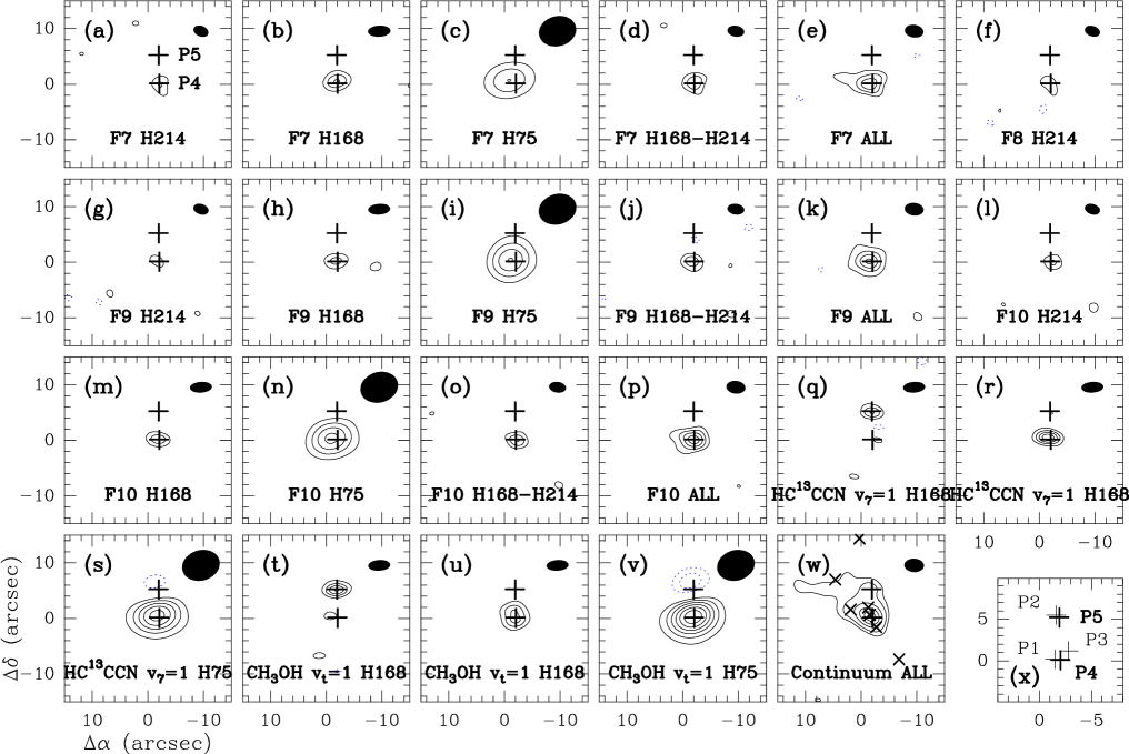
Since the line-free frequency ranges in the two spectral windows are too small to compute a reliable continuum map, we present in Fig. 8w a map combining the emission obtained at 93.2 and 97.4 GHz in the continuum mode. The contaminating lines were avoided in the integration. The continuum emission detected with the ATCA has properties very similar to the emission detected with the PdBI (see Sect. 3.4). The emission peaks at , , i.e. within 0.3 of the ultracompact Hii region K2 (Gaume et al. 1995). The continuum emission is somewhat extended around the main peak: it extends toward the other ultracompact Hii regions K1, K3, and the shell-like Hii region K5, but these features are not resolved with the ATCA. We also detect a shell-like emission close to K6, but its signal-to-noise ratio is lower than in the PdBI data. We do not detect any emission toward the weak ultracompact Hii region K9.69 (Gaume et al. 1995).
The strong methanol vt=1 and HC13CCN v7=1 lines show the same structure as the strong lines detected with the PdBI, namely emission from two different positions separated by about 5.1 in declination, each with a distinct velocity (Fig. 8q, r, t, and u). These two positions P4 and P5 coincide with the PdBI positions P1 and P2, respectively, within 0.5 which is about one fifth of the ATCA synthesized beam (see Fig. 8x for a visual comparison). Therefore we are very confident that they correspond to the same regions. The third position P3 detected with the PdBI in methylformate is not detected in the small number of transitions observed with the ATCA.
Within the limits of our sensitivity, the amino acetonitrile features F7 to F10 show only one peak, and they all peak at the same position P4 coincident with the PdBI position P1. Therefore, all amino acetonitrile features detected with both the ATCA and the PdBI peak at the same position, which is consistent with their assignment to the same molecule. The emission detected in features F7 to F10 is barely resolved with the ATCA. Given the uncertainties, it is consistent with the source size of 2 suggested by our measurements with the PdBI. The ATCA spatially integrated flux of feature F7 in the mixed configuration H 214 + H168 agrees with the 30m telescope flux within 40. Given the calibration uncertainties of both instruments, and the somewhat larger noise in the 30m spectrum, most of the flux of feature F7 is recovered with the ATCA. On the other hand, the ATCA spatially integrated fluxes of features F8 to F10 are significantly weaker than the 30m telescope fluxes. The main reason for this disagreement may be the contamination of the 30m spectrum by emission from transitions of other molecules which are still unidentified in our survey (see Fig. 7l). This contaminating emission is missed by the interferometer either because it peaks at an offset position or because it is extended and filtered out.
The model spectrum of amino acetonitrile computed with the same parameters as the 30m model (see Table 5) but with the spatial resolution of the ATCA is shown in red in Fig. 7a to j. The agreement with the spectra obtained with the ATCA is good, within a factor of 2 (see comment about the interferometric modeling in Sect. 3.4). Overall, our LTE model of amino acetonitrile is therefore well consistent with the compact emission detected with the ATCA.
3.6 Abundance of amino acetonitrile in Sgr B2(N)
The continuum emission detected with the PdBI (see Fig. 6o) has a peak intensity of Jy/-beam. In the 2”-diameter region convolved by the PdBI beam centered on the AAN peak position P1 (convolved FWHM: ), we measure a mean intensity of 0.257 Jy/beam and a flux of 0.556 Jy. The continuum emission from Sgr B2(N) at 3.7 mm is dominated by thermal dust emission, at most 30 come from free-free emission (Kuan et al. 1996), probably even less toward the ultracompact Hii region K2 since its flux is only 20 and 60 mJy at 2 and 1.3 cm, respectively (Gaume & Claussen 1990; Gaume et al. 1995). In addition, the thermal dust emission is optically thin (Carlstrom & Vogel 1989), so we can estimate the H2 column density using the equation:
| (1) |
with the intensity at GHz, rad2 the solid angle of the synthesized beam, the mean molecular weight, the mass of atomic hydrogen, the dust mass opacity (for a standard gas-to-dust ratio of 100 by mass), and the Planck function at the dust temperature . We assume a dust mass opacity (230 GHz) = 0.01 cm2 g-1 valid for dust grains that have coagulated at high density and acquired ice mantles (Ossenkopf & Henning 1994) and a dust emissivity exponent , which yield a dust mass opacity (82 GHz) = 0.0036 cm2 g-1. Since gas and dust are well thermally coupled via collisions at densities above cm-3 (see, e.g., Lesaffre et al. 2005), we assume a dust temperature equal to the excitation temperature derived for amino acetonitrile (100 K, see Table 5 and Fig. 3). We obtain a mean H2 column density cm-2 in the inner region where we detect the amino acetonitrile emission with the PdBI. Assuming a distance of 8 kpc (see Sect. 1.1), the central region of deconvolved FWHM diameter 2 has a linear diameter of 16000 AU. We derive a total mass of 2340 M⊙ from its integrated flux (0.556 Jy). Assuming spherical symmetry, this translates into a mean density cm-3.
Using the column density derived from our modeling (see Table 5), we find an amino acetonitrile abundance relative to H2 of about in the inner region of deconvolved FWHM diameter 2, with an uncertainty on the abundance of at least a factor of 2 given the uncertainties on the dust mass opacity and the dust emissivity exponent.
The continuum emission detected with the ATCA at a mean frequency of 95.3 GHz has a peak intensity of 1.00 Jy/-beam. This intensity is 1.8 times larger than the PdBI continuum flux measured over an area (see above). If this flux difference comes from the frequency dependence of the continuum emission, then we derive a frequency exponent of 3.9 which is, within the calibration uncertainties, consistent with the exponent of 3.5 expected for thermal dust emission with a dust emissivity exponent assumed above. We are therefore confident that the continuum emission detected toward K2 with the PdBI and the ATCA is largely dominated by thermal dust emission.
3.7 Limits on possible extended emission of cold amino acetronitrile with the VLA
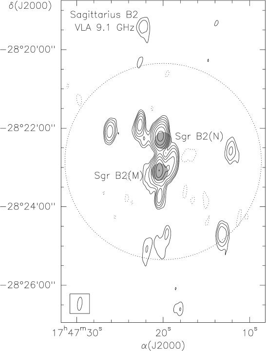
Figure 9 shows the continuum image of the Sgr B2 region we obtained at 9.1 GHz with the VLA. At this frequency, the primary beam has a FWHM of . Our -data should adequately sample structures with sizes of up to . There are two major continuum sources, Sgr B2(N) and (M), whose emission is a blend of the contributions of many separate sources that are resolved in higher resolution images (e.g., Gaume et al. 1995). A number of secondary sources are evident. The peak brightness, , toward Sgr B2(N) is 2.85 Jy beam-1. Toward Sgr B2(M) we measure Jy beam-1. The image has a relatively high 1 rms noise level of 8.4 mJy beam-1 that is determined by dynamic range limitations. Nowhere in the whole line datacube do we find any significant line emission or absorption above 3.4 mJy beam-1 (5 times the 1 rms noise level in the images of the spectral line emission). This corresponds to a brightness temperature upper limit of 0.35 K. With this, and assuming a width of 30 km s-1, similar to other lines with extended emission (e.g., Hunt et al. 1999; Hollis et al. 2004) we can use the standard relation to calculate an upper limit to the column densities of the upper levels of the strongest of the hfs components of cm-2. Hollis et al. (2004) use a two temperature component picture to explain their multitransition glycolaldehyde study, invoking components with temperatures of and 50 K. For 8 K, our limit on the total column density of extended amino acetonitrile would be cm-2 and for 50 K it would be cm-2. The low- value is on the same order as the total column density of glycolaldehyde that Hollis et al. (2004) calculate for this temperature.
Using the ATCA, Hunt et al. (1999) imaged Sgr B2 in the line of HC3N at a frequency near 9.1 GHz, very close to our amino acetonitrile frequency. In their resolution images they found the spatial distribution of the line emission to resemble that of the continuum emission very closely. Assuming that possible extended amino acetonitrile had a similar distribution, the high continuum flux densities allow us to determine very sensitive limits on possible absorption (or weakly inverted emission) toward the continuum emission. We calculate very low limits on the absolute value of the optical depth of and toward Sgr B2(N) and (M). This implies and 20 times lower column density limits for and 50 K, respectively, compared to limits on possible thermal emission quoted above.
4 Discussion
4.1 Amino acetonitrile in Sgr B2(N)
We detected compact emission from amino acetonitrile in Sgr B2(N) with a source size of 2 FWHM, a column density of cm-2, an excitation temperature of 100 K, a linewidth of 7 km s-1, and a centroid velocity of 64 km s-1 (see Table 5). We estimated the abundance of amino acetonitrile to be in this compact region. We found no evidence for a possible colder, more extended emission. The compact emission peaks at position P1 (see Sect. 3.4 and Table 7), which is located 0.4 South of the ultracompact Hii region K2 where the 3.7 mm thermal dust continuum emission detected with the PdBI also peaks. This angular separation is at a level of 2 only, so it may not be significant. Our PdBI and ATCA data show that ethyl cyanide C2H5CN, cyanoacetylene HC3N in its excited states v and v, HC13CCN in its excited state v, and methanol CH3OH in its excited state v also peak at this position P1. The amino acetonitrile emission arises therefore from the hot core region called the “Large Molecule Heimat” (see Sect. 1.1.2). Our PdBI continuum data show that this compact region is extremely dense ( cm-3) and massive (2340 M⊙). The ultracompact Hii region K2 is most likely still embedded in the dense, hot core traced by the thermal dust emission and seems therefore to be the youngest source among the numerous ultracompact Hii regions populating the Sgr B2 molecular cloud. In addition, the LMH hosts the powerful Sgr B2(N) H2O maser region. The distribution of the maser emission over was mapped using Very Long Baseline Interferometry by Reid et al. (1988), who also fitted a kinematical model invoking expansion and rotation. The best fit center of expansion is displaced from our interferometric position P1 by () = (), which is less than the combined positional uncertainty of the VLBI and PdBI data. The best fit radial component of the expansion velocity, km s-1, is also in excellent agreement with the 64 km s-1 that we obtain for the LMH (see Table 5). H2O masers are associated with young stellar objects in their earliest stages when they drive powerful outflows, such as the one found in Sgr B2(N) which has a total velocity extent of km s-1 (see, e.g., Reid et al. 1988). Thus, the water vapor maser provides evidence for the youth of the LMH, the very compact region where the amino acetonitrile emission originates from.
Bisschop et al. (2007) measured the abundances of various complex molecules in massive hot core regions and classified these molecules as “cold” ( K) or “hot” ( K). Based on the high abundances, the similar high rotation temperatures, and the relative constant abundance ratios of the oxygen-bearing species and two nitrogen-bearing species, they concluded that the “hot” molecules share a common solid state formation scheme. From an analysis of the emission of complex organic molecules in molecular clouds in the Galactic center region and a comparison to results previously obtained in hot cores, Requena-Torres et al. (2006) support also the scenario in which complex organic molecules are formed on the grain surfaces. The high temperature and abundance we measured for amino acetonitrile suggest it shares the same properties as the “hot” molecules found by Bisschop et al. (2007), which favors its formation on the grain surfaces, although its detection in other hot cores to check if it follows the abundance correlations found by Bisschop et al. (2007) and Requena-Torres et al. (2006) is needed to prove this conclusion.
Wirström et al. (2007) failed to detect amino acetonitrile in the hot cores Orion~KL, W51~e1$/$e2, S140, and W3(OH) with the Onsala 20m telescope. They found beam-averaged column density upper limits of cm-2 for amino acetonitrile, while they detected vinylcyanide C2H3CN with a column density of cm-2 in the first two sources. Our 30m observations of Sgr B2(N) imply a column density of cm-2 for vinylcyanide with a source size of 2.3 (Belloche et al., in prep.), i.e. about 30 times our amino acetonitrile column density. If the column density ratio of these two species in Sgr B2(N) holds for other hot cores, then the observations of Wirström et al. (2007) were not sensitive enough to detect amino acetonitrile in their sources.
Our PdBI and ATCA data show that the double peak structure seen in many transitions detected with the 30m telescope are produced by two sources separated by about 5.3 in the North-South direction (positions P1 and P2, see Sect. 3.4). The centroid velocity difference between these two positions is about 9 km s-1. The northern and more redshifted source (P2) is about twice weaker in the molecular emission detected in our 30m data (Belloche et al., in prep.). These two sources were already detected in ethylcyanide with high-resolution observations (see, e.g., Liu & Snyder 1999; Hollis et al. 2003; Jones et al. 2007). Our interferometric data show that cyanoacetylene HC3N and its isotopologue HC13CCN in their excited state v, and methanol in its excited state v are also detected toward both sources. In the PdBI spectra shown in Fig. 5c and d, we do not find a clear evidence for amino acetonitrile at a velocity of km s-1. There may be a hint of emission at a level about a factor of 2 lower than the emission toward P1 (see also Feature F3 in the 30m spectrum in Fig. 5g), but it is below our 3 detection limit. Therefore we cannot rule out that amino acetonitrile shares the same property as, e.g., ethylcyanide, cyanoacetylene, and methanol and is also present in the northern source P2 at a level about twice lower than in P1.
The molecular source P2 is not detected at a 3 level of 26 mJy/-beam in the continuum map we obtained with the PdBI at 82.0 GHz (see Fig. 6o). On the other hand, we detect some emission with an intensity of 280 mJy/-beam in the continuum map obtained with the ATCA at a mean frequency of 95.3 GHz (see Fig. 8w). If this emission is more extended than the PdBI beam, then the PdBI upper limit translates into 79 mJy in the ATCA beam, which yields an unphysical frequency exponent of for the continuum emission toward P2 (see Sect. 3.6). We suspect that the ATCA continuum toward P2 is contaminated by a low-level line emission. In any case, since the continuum emission toward P2 is much weaker than toward P1 at 3mm, P2 must be less dense and/or less hot than the hot core P1. P2 coincides with a weak blob of emission in the 1.3 cm VLA map of Gaume et al. (1995) (see their Fig. 6 and 7). However, this blob is located within the shell-like, weak, extended emission associated with K5 and it is difficult to know if it is compact or not from the 1.3 cm map published by these authors. Therefore the hot core P2 traced by the molecular emission may also be associated with an ultracompact Hii region, weaker than K2. Alternatively, if it is not directely associated with a compact source of free-free emission, it may have been formed by the interaction of the shell-like structure K5 with the ambient medium, and could be in an earlier stage of evolution than the hot core P1 (LMH) associated with the ultracompact Hii region K2.
4.2 Amino acetonitrile in Sgr B2(M)
We do not detect amino acetonitrile in our 30m survey toward Sgr B2(M). Using the same parameters as for Sgr B2(N) (100 K and a FWHM source size of ), we find a column density upper limit of cm-2 in the LTE approximation. The column density of amino acetonitrile is thus at least a factor 5 weaker toward Sgr B2(M) than toward Sgr B2(N). This is not surprising since, e.g., Nummelin et al. (2000) found that hot-core-type molecules are more abundant in Sgr B2(N) by factors 3–8 as compared to Sgr B2(M).
4.3 Amino acetonitrile, a precursor of glycine?
Amino acids, building blocks of proteins and therefore key ingredients to explain the origin of life, have been found in meteorites on Earth. Their deuterium isotopic composition suggests that they, or at least their direct precursors, were formed in the cold interstellar medium (e.g. Pizzarello & Huang 2005). Looking for amino acids in the interstellar medium is therefore appealing. However, the simplest amino acid glycine has been intensively searched for in the past 30 years, but has unfortunately not been discovered yet (e.g. Brown et al. 1979; Snyder et al. 2005; Cunningham et al. 2007).
Amino acetonitrile was proposed early on as a possible direct precursor of glycine in the interstellar medium (e.g. Brown et al. 1977). The formation of glycine via a Strecker-cyanohydrin synthesis has long been favored (Peltzer et al. 1984; Ehrenfreund et al. 2001; Bernstein et al. 2004). This pathway involves a carbonyl compound (such as an aldehyde or a ketone), hydrogen cyanide, and ammonia, and produces the amino nitrile which, after hydrolysis, yields the amino acid. However, the Strecker synthesis cannot explain the higher deuterium fractionation of amino acids compared to hydroxy acids which was measured in meteorites (see Elsila et al. 2007 and references therein).
Amino acids were successfully produced in the laboratory by UV-photolysis of ice mixtures mimicking the mantles of insterstellar grains (Bernstein et al. 2002; Muñoz Caro et al. 2002). For an ice mixture composed of H2O, CH3OH, NH3, and HCN, Woon (2002) proposed theoretically a pathway of radical-radical reactions involving the radicals t-HOCO and CH2NH2 produced by UV irradiation. This hypothesis was tested and verified experimentally by Holtom et al. (2005) with an ice mixture of CH3NH2 and CO2 bombarded by energetic electrons mimicking the impact of cosmic rays in the interstellar medium. This pathway leading to glycine does not involve the formation of amino acetonitrile. On the other hand, Elsila et al. (2007) experimented the UV-photolysis of an ice mixture of H2O, CH3OH, HCN, and NH3, and found with isotopic labeling techniques multiple pathways leading to the formation of amino acids. The main pathway involves the formation of the amino nitrile and they proposed “a modified radical-radical mechanism that takes into account the formation of nitriles as amino acid precursor molecules”. They also noticed that a Strecker-type synthesis may be at most a minor contributor to the formation of glycine.
The formation of glycine in the gas phase was also investigated. Blagojevic et al. (2003) synthesized ionized glycine via the reaction of the hydroxylamine ion NH2OH+ with acetic acid CH3COOH. They proposed the formation of the precursor hydroxylamine NH2OH in the grain mantles and the formation of acetic acid via ion-molecule reactions in the gas phase. Based on quantum chemical calculations, Maeda & Ohno (2006) found another pathway to form glycine in the gas phase involving barrierless reactions between closed-shell species. Their pathway starts from CO2, NH3, and CH2, and leads to glycine via the reaction of CO2 with the closed-shell molecule CH2NH3, a higher energy isomer of methylamine CH3NH2. However, they mentioned that CH2NH3 should be efficiently destroyed by H2O, so this pathway may be unlikely in the interstellar gas phase where water can be very abundant. Both gas phase formation routes do not involve amino acetonitrile as a direct precursor of glycine.
This brief overview of the experimental and theoretical work on the formation of amino acids in the interstellar medium shows that there is no consensus about the chemical precursors of amino acids. It is however important to note that the amino acids produced in the ice experiments mentioned above (except Holtom et al. 2005) are found experimentally after the hydrolysis of the ice residues. It is possible that only their precursors (e.g. amino nitriles) are synthesized by the ice photochemistry, and that the amino acids are formed only later, e.g. on the comet/asteroids surfaces, by hydrolysis (Elsila et al. 2007). Therefore amino acetonitrile may well be a direct precursor of glycine.
The formation of amino acetonitrile itself was also investigated theoretically by Koch et al. (2008). They found that water can efficiently catalyze a reaction between methylenimine CH2NH and hydrogen isocyanide HNC to form amino acetonitrile in the grain mantles at a temperature of 50 K. Methylenimine was detected in the gas phase toward Sgr B2(N) by, e.g., Nummelin et al. (2000). They found evidence for both hot, compact and cold, extended components and derived a column density of cm-2 for the compact component, with a source size of 2.7 and a temperature of K, which is consistent with our own analysis (Belloche et al., in prep.). This column density is an order of magnitude larger than the column density we derived for amino acetonitrile, which does not rule out methylenimine as a precursor of amino acetonitrile.
4.4 Glycine in Sgr B2(N)
The frequency coverage of our 30m survey of Sgr B2(N) includes many transitions of glycine as listed in the CDMS catalog (entries 75511 and 75512), but we do not detect this molecule within the limits of our LTE analysis. Using the same parameters as for amino acetonitrile (100 K and a source size of 2, see Table 5), we derive a column density upper limit of cm-2 for conformer I and cm-2 for conformer II. Alternatively, the upper limit on emission from glycine more extended than the 30m beam at 3mm () is cm-2 for conformer I and cm-2 for conformer II. For a temperature of 75 K, we find column density upper limits for conformer I of cm-2 for a source size of 2 and cm-2 for emission more extended than the 30m beam, and for conformer II cm-2 and cm-2, respectively.
Jones et al. (2007) did not detect glycine conformer I in Sgr B2(N) with the ATCA and derived a 3 upper limit of cm-2 for the beam-averaged column density at 75 K, which translates into an upper limit of cm-2 for a source size of 2 after correction for beam dilution (). This upper limit on any compact emission from glycine is at a level 8 times lower than the one we derive with the 30m telescope. As Jones et al. (2007) mentioned, the tentative detection of Kuan et al. (2003) is inconsistent with this upper limit in the case of compact emission. On the other hand, the ATCA non-detection does not exclude extended emission at the level found by Kuan et al. (2003) who reported a beam-averaged column density of cm-2 with the NRAO 12m telescope and a rotational temperature of 75 K. However Cunningham et al. (2007) did not detect glycine conformer I in Sgr B2(N) with the 22m Mopra telescope and derived a 3 upper limit of cm-2 for the beam-averaged column density at 75 K. This upper limit is at a level 2.4 times lower than our beam-averaged upper limit. However, their upper limit was derived for a position offset by 26 from the hot core position, so it only rules out emission from Sgr B2(N) more extended than in diameter. If glycine’s emission were centered on the hot core position with a diameter of , Mopra would have missed of the flux, and their upper limit would be cm-2. In that case, our upper limit is more significant, but not low enough to rule out the tentative detection reported by Kuan et al. (2003) if glycine is confined to a source size of . However, the arguments presented by Snyder et al. (2005) do rule out this case. As a conclusion, the upper limits of Cunningham et al. (2007), Jones et al. (2007), and Snyder et al. (2005) rule out emission of glycine conformer I at the level reported by Kuan et al. (2003) in Sgr B2(N) for any source size.
Cunningham et al. (2007) found an upper limit of cm-2 for the beam-averaged column density of glycine conformer II with Mopra toward the central position of Sgr B2(N). This upper limit is nearly a factor of 3 lower than the upper limit we derived above with the 30m telescope for extended emission. With the ATCA, Jones et al. (2007) found an upper limit of cm-2 for the beam-averaged column density, which translates into cm-2 for a source size of 2. This upper limit is again a factor of 3 lower than the upper limit we derived above with the 30m telescope for compact emission.
Bernstein et al. (2004) found experimentally that organic acids are less stable than organic nitriles against UV photodestruction but they concluded that in dense molecular clouds, the ratio nitrile to acid should be affected by less than a factor of 2 over the lifetime of the cloud. Therefore it could be instructive to compare the pairs methylcyanide/acetic acid (CH3CN/CH3COOH) and amino acetonitrile/glycine (NH2CH2CN/NH2CH2COOH). In our 30m line survey (Belloche et al., in prep.), we derive a column density ratio on the order of 200 for CH3CN/CH3COOH toward Sgr B2(N). If the two pairs are produced by similar chemical pathways yielding similar column density ratios, then we expect the glycine column density to be two orders of magnitude smaller than the amino acetonitrile column density, i.e. about cm-2 for a compact source of 2 diameter, which is nearly two orders of magnitude smaller than the upper limit derived above for glycine conformer I from the ATCA measurements of Jones et al. (2007), and a factor 5 smaller for conformer II. Therefore glycine emission may be well below the confusion limit in Sgr B2(N).
5 Conclusions
We used the complete 3 mm and partial 2 and 1.3 mm line surveys obtained with the IRAM 30m telescope toward the hot cores Sgr B2(N) and (M) to search for emission from the complex molecule amino acetonitrile. We carried out follow-up observations with the IRAM Plateau de Bure and ATCA interferometers at selected frequencies. We also looked for extended emission from cold amino acetonitrile with the VLA. We report the detection of amino acetonitrile toward the hot core Sgr B2(N)-LMH, which is the first detection of this molecule in the interstellar medium. Our main results and conclusions are the following:
-
1.
In the course of this work, we prepared an amino acetonitrile entry (56507) for the catalog of the Cologne Database for Molecular Spectroscopy (CDMS) using the laboratory transition frequencies reported by Bogey et al. (1990).
-
2.
88 of the 398 significant transitions of amino acetonitrile covered by our 30m line survey are relatively free of contamination from other molecules and are detected in the form of 51 observed features toward Sgr B2(N).
-
3.
Nine features out of 51 were followed-up upon and detected with the IRAM PdB and ATCA interferometers. The amino acetonitrile emission looks compact and we derive a source size of about 2 in diameter (FWHM).
-
4.
With a source size of 2 and an LTE analysis, we derive an amino acetonitrile column density of cm-2 for a temperature of 100 K and a linewidth of 7 km s-1.
-
5.
The compact continuum emission detected with the PdB interferometer yields a mean H2 column density cm-2 in the central region of diameter 2 for a temperature of 100 K, which implies a mean density cm-3, a mass of 2340 M⊙, and an amino acetonitrile fractional abundance of .
-
6.
The high abundance and temperature may indicate that amino acetonitrile is formed by grain surface chemistry.
-
7.
We detected emission from ethylcyanide C2H5CN, cyanoacetylene HC3N and its isotopologue HC13CCN in their v7=1 excited states, and methanol CH3OH in its excited state vt=1 in two compact sources toward Sgr B2(N). The two sources are separated by about in the North-South direction and by 9 km s-1 in velocity. They produce double peaked line shapes for many molecules detected in our 30m line survey. Only the southern source is detected with the PdBI in continuum emission. It is associated with the ultracompact Hii region K2 and a powerful H2O maser region, and must be very young. The northern source is weaker in molecular emission and must be less dense and/or less hot. It may be associated with a weaker ultracompact Hii region and may be in an even earlier stage of evolution. The sensitivity of our observations was not good enough to detect amino acetonitrile toward the northern source. It is at least a factor of 2 weaker than toward the southern source.
-
8.
We did not detect amino acetonitrile toward Sgr B2(M) and derived a column density upper limit of cm-2.
-
9.
We failed to detect any extended emission from cold amino acetonitrile with the VLA and derived a column density upper limit of cm-2 at 8 K.
-
10.
Amino acetonitrile may be a chemical precursor of glycine. We did not detect the glycine conformers I and II in our 30m line survey. The column density upper limits we derive are less constraining than upper limits previously published by other authors. Based on our detection of amino acetonitrile and a comparison to the pair methylcyanide/acetic acid (CH3CN/CH3COOH) both of which are detected in our survey, we conclude that the column density of glycine conformers I and II in Sgr B2(N) may be two orders of magnitude and a factor 5 below the current best upper limits, respectively, which would be below the confusion limit of Sgr B2(N) in the 1–3 mm range.
Acknowledgements.
We thank the IRAM staff in Grenoble for observing at the PdBI and for their help with the data reduction, the IRAM staff in Granada for service observing in January 2005, and Sergio Martin for providing the reference (off) position for our 30m observations. We thank John Pearson for his predictions of the first excited state of ethylcyanide, Claus Nielsen for providing transition frequencies of formamide isotopologues, Isabelle Kleiner, Vadim Ilyushin, and Frank Lovas for acetic acid frequencies, and Brian Drouin for his predictions of acetone. H. S. P. M. and the CDMS had been supported initially through the Deutsche Forschungsgemeinschaft (DFG) via the collaborative research grant SFB 494. Recent support is provided by the Bundesministerium für Bildung und Forschung administered through Deutsches Zentrum für Luft- und Raumfahrt (DLR; the German space agency). J. O. is a Jansky Fellow of the National Radio Astronomy Observatory. C. H. is a fellow of the Studienstiftung des deutschen Volkes and member of the International Max-Planck Research School for Radio and Infrared Astronomy.References
- Bernstein et al. (2002) Bernstein, M. P., Dworkin, J. P., Sandford, S. A., Cooper, G. W., & Allamandola, L. J. 2002, Nature, 416, 401
- Bernstein et al. (2004) Bernstein, M. P., Ashbourn, S. F. M., Sandford, S. A., & Allamandola, L. J. 2004, ApJ, 601, 365
- Berulis et al. (1985) Berulis, I. I., Winnewisser, G., Krasnov, V. V., & Sorochenko, R. L. 1985, Soviet Astronomy Letters, 11, 251
- Bisschop et al. (2007) Bisschop, S. E., Jörgensen, J. K., van Dishoeck, E. F., & de Wachter, E. B. M. 2007, A&A, 465, 913
- Blagojevic et al. (2003) Blagojevic, V., Petrie, S., & Bohme, D. K. 2003, MNRAS, 339, L7
- Bogey, Dubus, & Guillemin (1990) Bogey, M., Dubus, H., & Guillemin, J. C. 1990, J. Mol. Spectrosc., 143, 180
- Brown et al. (1977) Brown, R. D., Godfrey, P. D., Ottrey, A. L., & Storey, J. W. V. 1977, J. Mol. Spectrosc., 68 (3), 359
- Brown et al. (1979) Brown, R. D., Godfrey, P. D., Storey, J. W. V., Bassez, M.-P., et al. 1979, MNRAS, 186, 5P
- Carlstrom & Vogel (1989) Carlstrom, J. E., & Vogel, S. N. 1989, ApJ, 337, 408
- Ceccarelli et al. (2000) Ceccarelli, C., Loinard, L., Castets, A., Faure, A., & Lefloch, B. 2000, A&A, 362, 1122
- Clark (1980) Clark, B. G. 1980, A&A, 89, 377
- Combes et al (1996) Combes, F., Q-Rieu, N., & Wlodarczak, G. 1996, A&A, 308, 618
- Comito et al. (2005) Comito, C., Schilke, P., Phillips, T. G., Lis, D. C., Motte, F., & Mehringer, D. 2005, ApJS, 156, 127
- Cummins, Linke, & Thaddeus (1986) Cummins, S. E., Linke, R. A., & Thaddeus, P. 1986, ApJS, 60, 819
- Cunningham et al. (2007) Cunningham, M. R., et al. 2007, MNRAS, 376, 1201
- Dahmen et al. (1997) Dahmen, G., et al. 1997, A&AS, 126, 197
- de Vicente et al. (2000) de Vicente, P., Martín-Pintado, J., Neri, R., & Colom, P. 2000, A&A, 361, 1058
- Ehrenfreund et al. (2001) Ehrenfreund, P., Glavin, D. P., Botta, O., Cooper, G., & Bada, J. L. 2001, Proceedings of the National Academy of Science, 98, 2138
- Eisenhauer et al. (2003) Eisenhauer, F., Schödel, R., Genzel, R., Ott, T., Tecza, M., Abuter, R., Eckart, A., & Alexander, T. 2003, ApJ, 597, L121
- Elsila et al. (2007) Elsila, J. E., Dworkin, J. P., Bernstein, M. P., Martin, M. P., & Sandford, S. A. 2007, ApJ, 660, 911
- Gaume & Claussen (1990) Gaume, R. A., & Claussen, M. J. 1990, ApJ, 351, 538
- Gaume et al. (1995) Gaume, R. A., Claussen, M. J., de Pree, C. G., Goss, W. M., & Mehringer, D. M. 1995, ApJ, 449, 663
- Goldsmith & Langer (1999) Goldsmith, P. F., & Langer, W. D. 1999, ApJ, 517, 209
- Gordy & Cook (1984) Gordy, W., & Cook, R. L. 1984, Microwave Molecular Spectra, 3rd edition, Wiley (New York)
- Hollis et al. (1980) Hollis, J. M., Snyder, L. E., Suenram, R. D., & Lovas, F. J. 1980, ApJ, 241, 1001
- Hollis et al. (2000) Hollis, J. M., Lovas, F. J., & Jewell, P. R. 2000, ApJ, 540, L107
- Hollis et al. (2001) Hollis, J. M., Vogel, S. N., Snyder, L. E., Jewell, P. R., & Lovas, F. J. 2001, ApJ, 554, L81
- Hollis et al. (2002) Hollis, J. M., Lovas, F. J., Jewell, P. R., & Coudert, L. H. 2002, ApJ, 571, L59
- Hollis et al. (2003) Hollis, J. M., Pedelty, J. A., Boboltz, D. A., Liu, S.-Y., Snyder, L. E., Palmer, P., Lovas, F. J., & Jewell, P. R. 2003, ApJ, 596, L235
- Hollis et al. (2004) Hollis, J. M., Jewell, P. R., Lovas, F. J., Remijan, A., & Møllendal, H. 2004, ApJ, 610, L21
- Hollis et al. (2007) Hollis, J. M., Jewell, P. R., Remijan, A. J., & Lovas, F. J. 2007, ApJ, 660, L125
- Holtom et al. (2005) Holtom, P. D., Bennett, C. J., Osamura, Y., Mason, N. J., & Kaiser, R. I. 2005, ApJ, 626, 940
- Hunt et al. (1999) Hunt, M. R., Whiteoak, J. B., Cragg, D. M., White, G. L., & Jones, P. A. 1999, MNRAS, 302, 1
- Jones et al. (2007) Jones, P. A., Cunningham, M. R., Godfrey, P. D., & Cragg, D. M. 2007, MNRAS, 374, 579
- Jones et al. (2008) Jones, P. A., Burton, M. G., Cunningham, M. R., Menten, K. M., Schilke, P., Belloche, A., Leurini, S., Ott, J., Walsh, A. J. 2008, MNRAS, in press
- Koch et al. (2008) Koch, D. M., Toubin, C., Peslherbe, G. H., & Hynes, J. T. 2008, J. Phys. Chem. C, 112(8), 2972
- Kuan & Snyder (1996) Kuan, Y.-J., & Snyder, L. E. 1996, ApJ, 470, 981
- Kuan et al. (1996) Kuan, Y.-J., Mehringer, D. M., & Snyder, L. E. 1996, ApJ, 459, 619
- Kuan et al. (2003) Kuan, Y.-J., Charnley, S. B., Huang, H.-C., Tseng, W.-L., & Kisiel, Z. 2003, ApJ, 593, 848
- Lesaffre et al. (2005) Lesaffre, P., Belloche, A., Chièze, J.-P., & André, P. 2005, A&A, 443, 961
- Lis et al. (1991) Lis, D. C., Carlstrom, J. E., & Keene, J. 1991, ApJ, 380, 429
- Lis et al. (1993) Lis, D. C., Goldsmith, P. F., Carlstrom, J. E., & Scoville, N. Z. 1993, ApJ, 402, 238
- Liu & Snyder (1999) Liu, S.-Y., & Snyder, L. E. 1999, ApJ, 523, 683
- Liu et al. (2001) Liu, S.-Y., Mehringer, D. M., & Snyder, L. E. 2001, ApJ, 552, 654
- MacDonald & Tyler (1972) MacDonald, J. N. & Tyler, J. K. 1972, J. Chem. Soc. Chem. Comm., 995
- Maeda & Ohno (2006) Maeda, S., & Ohno, K. 2006, ApJ, 640, 823
- Mehringer et al. (1995) Mehringer, D. M., Palmer, P., & Goss, W. M. 1995, ApJS, 97, 497
- Mehringer & Menten (1997) Mehringer, D. M., & Menten, K. M. 1997, ApJ, 474, 346
- Mehringer et al. (1997) Mehringer, D. M., Snyder, L. E., Miao, Y., & Lovas, F. J. 1997, ApJ, 480, L71
- Menten (2004) Menten, K. M. 2004, in The Dense Interstellar Medium in Galaxies, Eds. Pfalzner, Kramer, Staubmeier, & Heithausen, Springer proceedings in physics, Vol. 91 (Berlin, Heidelberg: Springer), 69
- Miao et al. (1995) Miao, Y., Mehringer, D. M., Kuan, Y.-J., & Snyder, L. E. 1995, ApJ, 445, L59
- Miao & Snyder (1997) Miao, Y., & Snyder, L. E. 1997, ApJ, 480, L67
- Minh et al. (1992) Minh, Y. C., Irvine, W. M., & Friberg, P. 1992, A&A, 258, 489
- Morris & Serabyn (1996) Morris, M., & Serabyn, E. 1996, ARA&A, 34, 645
- Müller et al. (2001) Müller, H. S. P., Thorwirth, S., Roth, D. A., & Winnewisser, G. 2001, A&A, 370, L49
- Müller et al. (2005) Müller, H. S. P., Schlöder, F., Stutzki, J., & Winnewisser, G. 2005, J. Mol. Struct., 742, 215
- Muñoz Caro et al. (2002) Muñoz Caro, G. M., Meierhenrich, U. J., Schutte, W. A., Barbier, B., et al. 2002, Nature, 416, 403
- Nummelin et al. (2000) Nummelin, A., Bergman, P., Hjalmarson, Å., Friberg, P., Irvine, W. M., Millar, T. J., Ohishi, M., & Saito, S. 2000, ApJS, 128, 213
- Ossenkopf & Henning (1994) Ossenkopf, V., & Henning, T. 1994, A&A, 291, 943
- Peltzer et al. (1984) Peltzer, E. T., Bada, J. L., Schlesinger, G., & Miller, S. L. 1984, Advances in Space Research, 4, 69
- Pickett (1973) Pickett, H. M. 1973, J. Mol. Spectrosc., 46, 335
- Pickett (1991) Pickett, H. M. 1991, J. Mol. Spectrosc., 148, 371
- Pickett et al. (1998) Pickett, H. M., Poynter, R. L., Cohen, E. A., Delitsky, M. L., Pearson, J. C., & Müller, H. S. P. 1998 , J. Quant. Spectrosc. & Rad. Transfer, 60, 883
- Pizzarello & Huang (2005) Pizzarello, S., & Huang, Y. 2005, Geochim. Cosmoschim. Acta, 69, 599
- Reid (1993) Reid, M. J. 1993, ARA&A, 31, 345
- Reid et al. (1988) Reid, M. J., Schneps, M. H., Moran, J. M., Gwinn, C. R., Genzel, R., Downes, D., & Roennaeng, B. 1988, ApJ, 330, 809
- Remijan et al. (2002) Remijan, A., Snyder, L. E., Liu, S.-Y., Mehringer, D., & Kuan, Y.-J. 2002, ApJ, 576, 264
- Requena-Torres et al. (2006) Requena-Torres, M. A., Martín-Pintado, J., Rodríguez-Franco, A., Martín, S., Rodríguez-Fernández, N. J., & de Vicente, P. 2006, A&A, 455, 971
- Sault, Teuben, & Wright (1995) Sault, R. J., Teuben, P. J., & Wright, M. C. H. 1995, Astronomical Data Analysis Software and Systems IV, 77, 433
- Snyder, Kuan, & Miao (1994) Snyder, L. E., Kuan, Y.-J., & Miao, Y. 1994, Lecture Notes in Physics 439: The Structure and Content of Molecular Clouds, Eds. T. L. Wilson and K. J. ’ Johnston, Springer-Verlag, 439, 187
- Snyder et al. (2002) Snyder, L. E., Lovas, F. J., Mehringer, D. M., Miao, N. Y., Kuan, Y., Hollis, J. M., & Jewell, P. R. 2002, ApJ, 578, 245
- Snyder et al. (2005) Snyder, L. E., Lovas, F. J., Hollis, J. M., Friedel, D. N., et al. 2005, ApJ, 619, 914
- Storey (1976) Storey, J. W. V. 1976, Ph.D. Thesis, Monash University
- Turner & Apponi (2001) Turner, B. E., & Apponi, A. J. 2001, ApJ, 561, L207
- Vogel et al. (1987) Vogel, S. N., Genzel, R., & Palmer, P. 1987, ApJ, 316, 243
- Wirström et al. (2007) Wirström, E. S., Bergman, P., Hjalmarson, Å., & Nummelin, A. 2007, A&A, 473, 177
- Woon (2002) Woon, D. E. 2002, ApJ, 571, L177