An $\mathcal{O}(N^{2})$ Approximation for Hydrodynamic Interactions in Brownian Dynamics Simulations

Abstract

In the Ermak-McCammon algorithm for Brownian Dynamics, the hydrodynamic interactions (HI) between $N$ spherical particles are described by a $3N\times 3N$ diffusion tensor. This tensor has to be factorized at each timestep with a runtime of $\mathcal{O}(N^{3})$, making the calculation of the correlated random displacements the bottleneck for many-particle simulations. Here we present a faster algorithm for this step, which is based on a truncated expansion of the hydrodynamic multi-particle correlations as two-body contributions. The comparison to the exact algorithm and to the Chebyshev approximation of Fixman verifies that for bead-spring polymers this approximation yields about 95% of the hydrodynamic correlations at an improved runtime scaling of $\mathcal{O}(N^{2})$ and a reduced memory footprint. The approximation is independent of the actual form of the hydrodynamic tensor and can be applied to arbitrary particle configurations. This now allows to include HI into large many-particle Brownian dynamics simulations, where until now the runtime scaling of the correlated random motion was prohibitive.

I Introduction

For the simulation of diffusional processes on the scales of polymers or proteins, Brownian Dynamics has proven to be a reliable workhorse GAB02 ; GRO03 ; GOR04 ; SPA06 ; HER06 ; DLUG07 . This coarse grained method builds upon Einstein’s microscopic explanation of the random motion of colloidal particles EIN05 which had been observed earlier by the biologist Robert Brown when studying pollen grains. In Einstein’s explanation the solvent molecules are replaced by a heat bath that models the collisions between the solvent molecules and the much larger Brownian particles by correctly distributed random forces. Together with the assumption that the motion of the large observable particles is overdamped, i.e., that their velocities relax very fast compared to the time steps used in the simulation, their diffusive motion is reproduced DHO96 . Replacing the many small solvent molecules by a continuum dramatically reduces the computational costs compared to an all-atom molecular dynamics simulation, but for the price that also all interactions between the Brownian particles have to be adapted to include the effects of the now continuous solvent. For electrostatic interactions, e.g., the polarizability of the solvent molecules and the redistribution of the included ions can be described by an effective shielding via the Debye-Hückel theory. When the solvent molecules are not considered explicitly anymore, also so called hydrodynamic interactions (HI) have to be included, which describe how the relative motion of the Brownian particles is coupled mechanically via the displaced solvent.

Now there is a fundamental difference between the effect of the hydrodynamic coupling onto the direct interactions between the Brownian particles and the one onto their random motion. An external force acting on one of the particles accelerates this particle, which in turn leads to a displacement of the other particles, too, mediated by the displaced solvent molecules. Effectively, with hydrodynamics the effect of the external forces is increased and the dynamics is accelerated compared to a setup that does not consider hydrodynamics. In contrast, the random motion of the Brownian particles models the effect of the thermal fluctuations of the solvent molecules, the strength of which depends on the temperature of the system. Consequently, for a correct description of the overall diffusion the random kicks must have the same strength with and without hydrodynamics, i.e., whether the correlation due to the displaced solvent is considered or neglected. Consequently, when hydrodynamic interactions are included in a BD simulation, the random displacements still have (up to second order) the same (temperature dependent) magnitudes, but are correlated DEU71 . In a simulation, they now have to be determined from a factorization of the diffusion tensor of the complete system, which is numerically demanding.

In a BD simulation of $N$ particles using the Ermak-McCammon algorithm ERM78 , the hydrodynamically correlated random displacements are determined via a Cholesky factorization of the $3N\times 3N$ diffusion tensor, which results in a runtime of $\mathcal{O}(N^{3})$, while all the two-body interactions can be calculated in $\mathcal{O}(N^{2})$ runtime. For a many particle simulation with HI, one is therefore spending most of the time evaluating the correlated random displacements. For practical applications, this limits the number of particles to a few dozens, when HI is included, while without HI the dynamics of some thousand particles could be simulated in the same time. As the already approximated direct interactions are most important for the dynamics of most biologically interesting association and dissociation processes, the time consuming HI is often neglected MCG06 . For applications to polymers or the dynamics of DNA, however, it may be important to explicitly include HI in order to reproduce the correct dynamic behavior AHL01 ; ZHO06 ; SZY07 .

Considering that HI should on the one hand not be completely neglected, but on the other hand is only one out of a handful of interactions, there is an urgent need for faster algorithms to compute the hydrodynamic coupling in the random motion of many particle systems. Fixman proposed to use a Chebyshev approximation, which scales as $\mathcal{O}(N^{2.5})$, to factorize the diffusion coefficient FIX86b . A drastically simplified approach to HI is the effective mobility model by Heyes et al., which changes the diffusion coefficients of the Brownian particles according to the local density HEY95 . Such a model can obviously not reproduce the full correlation between the individual particles. Based on these ideas, Banchio and Brady developed an algorithm for infinite homogenous suspensions that scales as $\mathcal{O}(N^{1.25}\log N)$ for large $N$ BAN03 . Due to its mathematical complexity, this algorithm only performs well for very large numbers of particles. Consequently, when HI is to be considered in BD simulations, many current studies either use the original Cholesky factorization for smaller systems or Fixman’s Chebyshev approximation with its better runtime scaling for larger many particle scenarios HUA02 .

Here we present a conceptionally different approach to tackle the computationally expensive correlation of random motion in many-particle simulations. Whereas all previous improvements to the Ermak-McCammon algorithm only considered the factorization of the hydrodynamic tensor, we argue that in typical BD simulations all interactions are approximative anyhow. Consequently, even with the exact (and very time-consuming) HI, the system dynamics will not be exactly the same as in an experiment. Thus one may try to approximate the correlations of the random forces, too, and reduce their functional complexity without further perturbing the dynamics in the simulation. The central requirement for such an approximation is thus that it may not introduce any systematic drift.

This publication is organized as follows. Before we present our truncated expansion ansatz, we shortly review the standard Ermak-McCammon algorithm for BD simulations and how HI is treated there. We also give a short introduction to the Chebyshev expansion of the HI as introduced by Fixman. In section III we compare our ansatz to the well established methods of Ermak and Fixman, respectively. The main tests are the dynamics of a bead-spring dimer, which was used by Ermak and McCammon to verify their algorithm, and the behavior of bead-spring polymers of various lengths. The simulation results show that our ansatz reproduces about 95% of the correlations due to hydrodynamics at a runtime which scales quadratic with the bead number. We close with a summary and an outlook pointing out potential extensions and applications.

II Evaluating hydrodynamic interactions

II.1 The Ermak-McCammon algorithm and the Rotne-Prager tensor

In the often used Ermak-McCammon algorithm for Brownian Dynamics ERM78 ; DIC84 the total displacement $\Delta r_{i}$ of the $i$th particle during a timestep $\Delta t$ due to the external forces $F_{j}$ acting on all the particles and the random displacement $R_{i}$ is given by

$$\Delta r_{i}(\Delta t)=\sum_{j}\frac{D_{ij}F_{j}}{k_{B}T}\Delta t+\sum_{j}\frac{\partial D_{ij}}{\partial r_{j}}\Delta t+R_{i}(\Delta t)$$ (1)

The $3N\times 3N$ diffusion tensor $\mathbf{D}=(D_{ij})$ describes the hydrodynamic coupling between the $N$ particles with their three translational degrees of freedom. For the external forces, $\mathbf{D}$ is used directly, whereas the hydrodynamically correlated random displacements $R_{i}(\Delta t)$ are characterized only indirectly by the statistical moments of a vanishing average and a finite covariance, which is described by the corresponding entries of $\mathbf{D}$:

$$\langle R_{i}(\Delta t)\rangle=0,\qquad\langle R_{i}(\Delta t)R_{j}(\Delta t)\rangle=2D_{ij}\Delta t\,.$$ (2)

The most common forms for the diffusion tensor are the Oseen tensor KIR48 and the Rotne-Prager-Yamakawa tensor ROT69 ; YAM70 . For these approximations the second term of equation (1), which describes how the particles are dragged into regions of faster diffusion, vanishes.

For identical spheres of radius $a$, the $3N\times 3N$ Rotne-Prager-Yamakawa hydrodynamic tensor, which couples the translational displacements of the beads, consists of the following $3\times 3$ submatrices $\mathbf{D}_{ij}$, where $i$ and $j$ label two particles:

$$\mathbf{D}_{ii} = \frac{k_{B}T}{6\pi\eta a}\mathbf{I}$$ (3)

$$\mathbf{D}_{ij} = \frac{k_{B}T}{8\pi\eta r_{ij}}\left[(\mathbf{I}+\hat{r}_{ij}\otimes\hat{r}_{ij})+\frac{2a^{2}}{3r_{ij}^{2}}(\mathbf{I}-3\hat{r}_{ij}\otimes\hat{r}_{ij})\right]$$ (5)

$$\quad i\neq j\mbox{ and }r_{ij}\geq 2a$$

$$\mathbf{D}_{ij} = \frac{k_{B}T}{6\pi\eta a}\left[\left(1-\frac{9}{32}\frac{r_{ij}}{a}\right)\mathbf{I}+\frac{3}{32}\frac{r_{ij}}{a}\hat{r}_{ij}\otimes\hat{r}_{ij}\right]$$ (7)

$$\quad i\neq j\mbox{ and }r_{ij}<2a$$

This tensor is positive definite for all particle configurations. Dickinson et al. DIC84 later showed how rotational coupling can be included, too. A generalization of the Rotne-Prager-Yamakawa tensor for spheres of different radii was introduced by Garcia de la Torre GAR77b .

To determine the random displacements from equation (2), one needs to find $\mathbf{B}$ so that $\mathbf{D}=\mathbf{B}\mathbf{B}^{T}$. One possible solution, which was used by Ermak and McCammon, comes from a Cholesky factorization, giving $\mathbf{B}$ as an upper (lower) tridiagonal matrix. The random displacements are then determined as $\vec{R}=\mathbf{B}\vec{X}$ from a $3N$ dimensional vector $\vec{X}$ of normal distributed random numbers.

II.2 Fixman’s Chebyshev approximation

To avoid the computationally expensive Cholesky factorization of the hydrodynamic tensor used in the Ermak-McCammon algorithm, Fixman suggested in 1986 to approximate the square root of the diffusion tensor via Chebyshev polynomials FIX86b . Fortunately, the explicit calculation of this matrix is not necessary and the vector of correlated displacements can be determined iteratively by a series of matrix-vector multiplications up to the order $L$ of the expansion:

$$\vec{R} \approx \sum_{l=0}^{L}a_{l}\vec{x}_{l}$$ (8)

$$\vec{x}_{0} = \vec{X}$$ (9)

$$\vec{x}_{1} = [d_{a}\mathbf{D}+d_{b}\mathbf{I}]\cdot\vec{X}$$ (10)

$$\vec{x}_{l+1} = 2[d_{a}\mathbf{D}+d_{b}\mathbf{I}]\cdot\vec{x}_{l}-\vec{x}_{l-1}$$ (11)

The factors $d_{a}$ and $d_{b}$ are related to the range of eigenvectors $[\lambda_{min},\lambda_{max}]$ of $\mathbf{D}$ as

$$d_{a}=\frac{2}{\lambda_{max}-\lambda_{min}}\quad\mbox{ and }\quad d_{b}=\frac{\lambda_{max}+\lambda_{min}}{\lambda_{max}-\lambda_{min}}$$ (12)

For further details like the evaluation of the expansion coefficients $a_{l}$ we refer the readers to, e.g., Press et al.PRE97

To determine the necessary order $L$ of the Chebyshev approximation and to control whether the eigenvalue spectrum of $\mathbf{D}$ is bounded correctly, we followed the procedure of Jendrejack et al. JEN00 . They introduced the relative error $\epsilon_{f}$ ($E_{f}$ in their notation) derived from the approximated random displacements $\vec{R}$, the uncorrelated random numbers $\vec{X}$, and the diffusion tensor $\mathbf{D}$:

$$\epsilon_{f}=\sqrt{\frac{|\vec{R}\cdot\vec{R}-\vec{X}\mathbf{D}\vec{X}|}{\vec{X}\mathbf{D}\vec{X}}}$$ (13)

As $\vec{R}\cdot\vec{R}$ can be evaluated with negligible additional cost, we used $\epsilon_{f}$ to monitor the convergence of the Chebyshev iteration (11). When $\epsilon_{f}$ remained above the chosen threshold with the actual values of $L$, $\lambda_{min}$, and $\lambda_{max}$, $L$ was increased by three and $\lambda_{min}$ and $\lambda_{max}$ were recalculated. For the next iteration, $L=l_{max}+3$ was used, where $l_{max}$ is the index of the last term of the iteration (11) required to get $\epsilon_{f}$ below the chosen threshold. Following Jendrejack et al. JEN00 , $\epsilon_{f}$ was set to $10^{-3}$ if not otherwise noted. For this value the numerical results were sufficiently close to the results with the exact Cholesky factorization.

II.3 The truncated expansion ansatz

The two methods outlined above focus on factorizing $\mathbf{D}$. Compared to the exact Cholesky factorization, the numerical approximation of Fixman manages to efficiently get close to the exact value of the square root of the diffusion tensor. We now present an approximation tailored for practical applications of many particle simulations, which algorithmically treats the displacements from the external forces and from the random forces on an equal footing.

For such an approximation we start from equation (1). Neglecting the random displacements, the displacement along coordinate $i$ during $\Delta t$ is

$$\Delta r_{i}(\Delta t)=\sum_{j}\frac{D_{ij}F_{j}}{k_{B}T}\Delta t=\frac{D_{ii}\Delta t}{k_{B}T}F_{i}^{eff},$$ (14)

where we introduced the hydrodynamically corrected effective force $F_{i}^{eff}$:

$$F_{i}^{eff}=\sum_{j}\frac{D_{ij}}{D_{ii}}F_{j}$$ (15)

This reformulation is independent of the actual form of the hydrodynamic tensor.

For the random displacements, we now make an ansatz with the same structure, i.e., we also introduce a hydrodynamically corrected random force $f_{i}^{eff}$ acting on coordinate $i$ which is derived from the uncorrelated random forces $f_{j}$ that would act on each of the particles in the absence of HI. In this ansatz the displacements due to the random forces alone are given as

$$\Delta r_{i}(\Delta t)=\frac{D_{ii}\Delta t}{k_{B}T}C_{i}\sum_{j}\beta_{ij}\frac{D_{ij}}{D_{ii}}f_{j}=\frac{D_{ii}\Delta t}{k_{B}T}f_{i}^{eff}.$$ (16)

The structure of this ansatz, which effectively factorizes $\mathbf{D}$ into individual two-body contributions, is taken from equation (14). The scaling factor $C_{i}$ takes care that for each individual coordinate its unperturbed diffusion coefficient $D_{ii}$ is regained DEU71 , while $\beta_{ij}$ allows for different weights when $\sqrt{\mathbf{D}}$ is used instead of $\mathbf{D}$ in equation (15). As we will see later, there is an individual scaling factor $C_{i}$ for each of the coordinates, while, due to symmetry reasons, for the coefficients $\beta_{ij}$ we only need two different values for the diagonal $\beta_{ii}$ and for the off-diagonal $\beta_{ij}$ with $i\neq j$, respectively.

Now the parameters $C_{i}$ and $\beta_{ij}$ have to be determined such that the moments of the correlated displacements (2) are reproduced with only small deviations. For the uncoupled random forces we use

$$\langle f_{i}\rangle=0\quad\mbox{and}\quad\langle f_{i}\;f_{j}\rangle=\frac{2(k_{B}T)^{2}}{D_{ii}\Delta t}\delta_{ij}\,,$$ (17)

i.e., they reproduce the mean and covariance of the random displacements in the uncorrelated case.

With correlation, i.e., with hydrodynamic coupling, the vanishing average $\langle R_{i}\rangle$ is fulfilled straightforwardly from $\langle f_{i}\rangle=0$. For the covariance we start from the product of $\Delta r_{i}$ and $\Delta r_{j}$ according to equation (16):

$$\Delta r_{i}\Delta r_{j}=\left(\frac{\Delta t}{k_{B}T}\right)^{2}C_{i}C_{j}\sum_{k,l}\beta_{ik}\beta_{jl}D_{ik}D_{jl}f_{k}f_{l}$$ (18)

Inserting (17) leads to the condition

$$\langle r_{i}r_{j}\rangle=2\Delta tC_{i}C_{j}\sum_{k}\beta_{ik}\beta_{jk}\frac{D_{ik}D_{jk}}{D_{kk}}\stackrel{{\scriptstyle!}}{{=}}2D_{ij}\Delta t.$$ (19)

The terms with $k\neq l$ drop from the double sum, because the $f_{j}$ are uncorrelated. Requiring that the variance of equation (2) be reproduced DEU71 for $i=j$ allows us to determine the normalization constants $C_{i}$:

$$\left(\frac{1}{C_{i}}\right)^{2}=\sum_{k}\beta_{ik}^{2}\frac{D_{ik}^{2}}{D_{ii}D_{kk}}$$ (20)

Without loss of generality, we can set $\beta_{ii}=1$. Then, equation (16) reduces to the usual form in the limit of vanishing HI. In this case, also $C_{i}=1$ and the displacement $\Delta r_{i}(\Delta t)$ can be calculated with equation (14) from the sum of the random force $f_{i}$ and the external force $F_{i}$.

With $\beta_{ii}=1$, equation (20) can also be written as

$$\left(\frac{1}{C_{i}}\right)^{2}=1+\sum_{k\neq i}\beta_{ik}^{2}\frac{D_{ik}^{2}}{D_{ii}D_{kk}}\,,$$ (21)

where the term with $k=i$ was taken out of the sum.

With our ansatz (16) there is no set of coefficients which can be determined numerically efficiently, with which equations (2) can be fulfilled simultaneously. To determine the remaining off-diagonal coefficients $\beta_{ij}$, we therefore proceed by assuming that the hydrodynamic coupling is weak, i.e., that the off-diagonal entries $D_{ij}$ of the hydrodynamic tensor are much smaller than the individual diffusion coefficients $D_{ii}$. Then we can use $\sqrt{1+\epsilon}\approx 1+\epsilon/2$ to expand equation (21):

$$\frac{1}{C_{i}}\approx 1+\frac{1}{2}\sum_{k\neq i}\beta_{ik}^{2}\frac{D_{ik}^{2}}{D_{ii}D_{kk}}$$ (22)

Thus, the product $(C_{i}C_{j})^{-1}$ in equation 19 can be approximated as

$$\frac{1}{C_{i}C_{j}}\approx 1+\frac{1}{2}\sum_{k\neq i}\frac{\beta_{ik}^{2}D_{ik}^{2}}{D_{ii}D_{kk}}+\frac{1}{2}\sum_{l\neq j}\frac{\beta_{jl}^{2}D_{jl}^{2}}{D_{jj}D_{ll}}+\mathcal{O}\left(\frac{D_{ij}}{D_{ii}}\right)^{4}$$ (23)

i.e., a constant term plus terms that are quadratic and quartic in $D_{ij}/D_{ii}$. As we have the same $\beta_{ii}=\beta=1$ for all $i$, we also set all $\beta_{ij}$ for $i\neq j$ to the same value $\beta^{\prime}$. Without the quartic term, equation (23) then becomes

$$\frac{1}{C_{i}C_{j}}\approx 1+(N-1)\,\beta^{\prime 2}\epsilon^{2}$$ (24)

with the averaged relative coupling strength $\epsilon=\langle D_{ij}/D_{ii}\rangle$.

Starting directly from equation (19) we get the non-approximated relation

$$\frac{1}{C_{i}}\frac{1}{C_{j}}=\sum_{k}\beta_{ik}\beta_{jk}\frac{D_{ik}D_{jk}}{D_{kk}D_{ij}}.$$ (25)

On the rhs of this equation the two terms with $k=i$ and $k=j$ can be taken out of the sum. They are independent of the hydrodynamic coupling, while all other terms are of first order in $D_{ij}/D_{ii}$. With $\beta=1$ this yields:

$$\frac{1}{C_{i}}\frac{1}{C_{j}}=2\beta^{\prime}+(N-2)\beta^{\prime 2}\epsilon$$ (26)

Comparing equations (24) and (26) then gives the quadratic equation

$$\beta^{\prime 2}\left[(N-1)\epsilon^{2}-(N-2)\epsilon\right]-2\beta^{\prime}+1=0,$$ (27)

which can be solved for $\beta^{\prime}$:

$$\beta_{ij}=\beta^{\prime}=\frac{1-\sqrt{1-[(N-1)\epsilon^{2}-(N-2)\epsilon]}}{(N-1)\epsilon^{2}-(N-2)\epsilon}$$ (28)

We note that $\beta_{ij}$ according to the above equation is not defined in the case of absent HI. However, it converges to $\beta_{ij}=1/2$ for vanishing HI, i.e., for $\epsilon\to 0$, the value obtained from equation (27) for $\epsilon=0$.

The resulting approximation to the hydrodynamically coupled random displacements of equation (16) with the normalization constants $C_{i}$ given by (20) and the two weights $\beta_{ii}=1$ and $\beta_{ij}$ according to equation (28) has the same structure as the displacements due to the hydrodynamically coupled external forces in equation (14), resulting in the same runtime scaling of $\mathcal{O}(N^{2})$ for both the deterministic and the random contributions to $\Delta r_{i}$. Consequently, with this algorithm, which treats the external and the random forces on equal footing, HI can now be included in all those BD simulations where the direct interparticle forces can be computed—given our approximation is accurate enough for the chosen application.

II.4 Simulation details

To evaluate how our ansatz compares to the standard methods, we ran BD simulations of bead-spring polymers with $N=2\ldots 2000$ beads of radius $a$. The diffusion coefficient of the individual beads was set to $D_{0}=1$, thus defining the time scale. The beads were connected to their direct neighbors in the chain by harmonic springs with

$$V_{h}(x)=a_{h}(x-L)^{2}.$$ (29)

The potential minimum was varied for the dimer simulations and set to $L=3a$ for the polymer simulations. To prevent the beads from overlapping, a repulsive harmonic potential between all beads was used analogous to the setup of Ermak and McCammon ERM78 :

$$V_{c}(x)=a_{h}(x-2a)^{2}\quad\mbox{ for }\quad r<2a$$ (30)

The spring constant for both interactions was set to the rather stiff value of $a_{h}=50$ $k_{B}T/a^{2}$, with which we used a conservatively estimated integration timestep $\Delta t=0.001$.

The Cholesky factorization, the eigenvalue calculation, the matrix and vector operations as well as the generation of the random numbers were performed with the respective subroutines from the GNU scientific library GSL06 .

For simulations of shorter polymers of $N<70$, all simulation were started with the beads of the polymer aligned along the $x$ axis with a mutual separation $L=3$. Data analysis was started when the polymer had reached its coiled state. This transition was observed via the radius of gyration. For polymers with $N>70$, the equilibration was too slow with hydrodynamics included. For every chain length we therefore started a set of simulations without hydrodynamics and a longer timestep of $\Delta t=0.003$ and saved the final positions when the polymer had coiled up. These snapshots were then used as starting points for simulations with the different forms of HI.

III Comparison of the methods

In the following section we evaluate how our truncated expansion approximation to HI (TEA-HI) compares to the other methods, namely the exact factorization of Ermak and McCammon and the Chebyshev approximation introduced by Fixman. For this, we analyzed the correlation coefficient of two random displacements in one dimension, the dynamics of a dimer, which had been introduced as a test case by Ermak and McCammon ERM78 , and several static and dynamic properties of bead-spring polymers. These comparisons will confirm that most of the hydrodynamic interaction is obtained with our approximation at a greatly improved runtime scaling.

III.1 Correlation coefficient

The simplest test is to directly evaluate the correlation coefficient $\rho_{ij}$ of two one-dimensional displacements that are hydrodynamically coupled:

$$\rho_{ij}=\frac{\langle\Delta r_{i}\,\Delta r_{j}\rangle}{\langle\Delta r_{i}\rangle\langle\Delta r_{j}\rangle}$$ (31)

For $D_{11}=D_{22}$, $D_{12}=D_{21}$ was varied between 0 and $D_{11}$ and $\rho_{ij}$ was averaged for correlated displacements using both the explicit Cholesky factorization and our approximation. For the whole range of $D_{12}$, our TEA-HI gave values for $\rho_{12}$, which were by less than 0.1% smaller than with the exact factorization. Similar minor deviations were obtained, too, for all tested cases with $D_{11}\neq D_{22}$.

III.2 Dimer dynamics

$L$	$\langle d\rangle$			$D_{CM}$				$\alpha_{D}$
			Geyer	Ermak	theo.		Geyer	Ermak	theo
2	2.028		0.7164	0.7468	0.7464		2.43	2.28	2.28
3	3.003		0.6530	0.6665	0.6665		2.97	2.93	2.93
4	4.002		0.6175	0.6253	0.6249		3.27	3.27	3.22
8	8.001		0.5612	0.5627	0.5625		3.59	3.59	3.62
20	20		0.5247	0.5243	0.5250		3.85	3.92	3.85
66.7	66.7		0.5073	0.5073	0.5075		3.92	3.91	3.96

Table 1: Comparison of the center-of-mass diffusion coefficient $D_{CM}$ and the rescaled correlation time $\alpha_{D}$ of the orientation of a dimer of spherical beads with radius $a$ connected by a spring of length $L$ from BD simulations with HI to their respective theoretical values. The actual average separation during the simulation is given by $\langle d\rangle$ and was used to calculate the theoretical predictions from (32) and (33). The headings “Geyer” and “Ermak” denote the respective type of HI that was used in the simulations.

In their original work ERM78 , Ermak and McCammon verified their approach to BD with HI by comparing the numerically determined diffusion coefficient of the center of mass of a dimer of spherical beads with radius $a$ and separation $L$, $D_{CM}$, and the inverse of the rescaled relaxation time of its orientation, $\alpha_{D}$, to analytical results. Only translational coupling between the beads was considered with the Rotne-Prager tensor. According to Ermak and McCammon ERM78 , with this form of the HI, the analytical values for $D_{CM}$ and $\alpha_{D}=T_{D}/\tau_{D}$ are

$$D_{CM} = \frac{D_{0}}{2}\left(1+\frac{a}{d}\right)$$ (32)

$$\alpha_{D} = 4\left(1-\frac{3a}{4d}-\frac{1}{2}\left(\frac{a}{d}\right)^{3}\right)$$ (33)

Here, $d$ is the distance between the centers of the two beads. $D_{CM}$ is given in units of the diffusion coefficient $D_{0}$ of a single bead. The relaxation time $\tau_{D}$ is given in units of $T_{D}=d^{2}/D_{0}$, which is the time that a single bead would need to diffuse over the separation $d$ between the two beads of the dimer. Without HI, the limiting values are $D_{CM}=0.5$ and $\alpha_{D}=4$.

In a spring-bead dimer the average distance between the two beads is slightly larger than the length $L$ of the spring connecting them. We therefore calculated $D_{CM}$ and $\alpha_{D}$ from the observed average separation $\langle d\rangle$ during the simulation for different spring lengths $L$. As seen in table 1, our results reproduce the analytical values for both $D_{CM}$ and $\alpha_{D}$ quite well. The hydrodynamic coupling tends to be underestimated by less than 7% for touching spheres, where the correlation is strongest, and much less for larger separations. Underestimating the HI has the consequence that the diffusion coefficient $D_{CM}$ is slightly smaller than the theoretical value and the relaxation time is slightly shorter, resulting in a larger $\alpha_{D}$. For comparison, table 1 also gives the numerical results for $D_{CM}$ and $\alpha_{D}$ with the correct factorization of Ermak and McCammon. Their deviation from the theoretical predictions is less than 2% which indicates the numerical uncertainties of the simulation results.

III.3 Static properties of bead-spring polymers

Figure 1: Average radius of gyration $\langle R_{g}^{2}\rangle$ (diamonds) and end-to-end distance $\langle R_{ee}^{2}\rangle$ (points) for polymers of various chain lengths $N$ from simulations where HI was calculated with Fixman’s Chebyshev approximation (open symbols) and with our truncated expansion approximation (filled symbols), respectively. The lines indicate the theoretically predicted scaling $\propto(N-1)^{1.176}$.

In the next two sections we present results from simulations of bead-spring polymers of various chain length $N$. Here we look at the equilibrium values of the radius of gyration $\langle R_{g}^{2}\rangle$ and the end-to-end $\langle R_{ee}^{2}\rangle$ distance. These are given by

$$\langle R_{g}^{2}\rangle=\frac{1}{2N^{2}}\sum_{ij}\langle r_{ij}\rangle$$ (34)

and

$$\langle R_{ee}^{2}\rangle=\langle(\vec{r}_{N}-\vec{r}_{1})^{2}\rangle.$$ (35)

Their theoretically predicted scaling behavior is

$$\langle R_{g}^{2}\rangle\propto\langle R_{ee}^{2}\rangle\propto(N-1)^{2\nu}$$ (36)

In a good solvent, perturbation analysis LI95 ; DUN02 predicts an exponent of $\nu\approx 0.588$ for $N\to\infty$, which is also reproduced in our simulations as shown in figure 1. For clarity, figure 1 only reproduces the results obtained with Fixman’s Chebyshev approximation and with our TEA-HI. Using the original Cholesky factorization of Ermak and McCammon or no HI at all gave results that were, within the numerical fluctuations, indistinguishable from the ones shown. However, for runtime reasons we only ran simulations for $N\leq 70$ with Ermak’s original method.

Over the range of chain lengths $N=4\ldots 200$, we obtained a ratio of $\langle R_{ee}^{2}\rangle/\langle R_{g}^{2}\rangle\approx 6.8$, which is about 10% larger than the results of Li et al. LI95 , Jendrejack et al. JEN00 , or Liu and Dünweg LIU03 . The difference may be due to the fact that in our simulations the ratio between bond length $L$ and bead radius $a$ is smaller than used there. Consequently, the polymer can not be compacted as much as with relatively smaller beads.

Even as the correct $\langle R_{g}^{2}\rangle$ and $\langle R_{ee}^{2}\rangle$ do not directly prove that our truncated expansion HI is correct, they show that it does not introduce any static perturbations to the polymer conformations.

III.4 Dynamic measures of bead-spring polymers

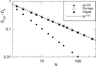
Figure 2: Diffusion coefficient $D_{cm}$ of the center of mass of bead-spring polymers of various chain lengths $N$ from simulations without HI (diamonds) and with HI using Fixman’s Chebyshev approximation (open points) or our truncated expansion approximation (filled points). The dashed line indicates the observed scaling of $N^{-0.56}$.

A central dynamic property of a diffusing polymer is its center of mass diffusion coefficient $D_{cm}$, which is predicted to scale as $D_{cm}\propto N^{-\nu}$ with $\nu\approx 0.588$ with Rotne-Prager HI and $\propto 1/N$ without HI. The scaling without HI was reproduced in our simulations, as can be seen in figure 2, which gives $D_{cm}$ in units of the diffusion coefficient $D_{0}$ of an individual bead. Without HI, the results are only shown up to $N=100$, but were calculated for $N=2\dots 400$.

With HI, the results with the original method of Ermak and McCammon and with Fixman’s approximation for $N=2\ldots 70$ were indistinguishable within the numerical uncertainties. For $N>70$, only the faster Chebyshev approximation was used. $D_{cm}$ from these simulation can be fitted well with $N^{-0.56}$, which means that in our simulations the diffusion of long polymers was slightly faster than predicted theoretically.

The results with our TEA-HI show the same scaling behavior, while $D_{cm}$ is slightly smaller than with the correct factorization of $\mathbf{D}$. The relative deviation between the results with our approach vs. the Chebyshev approximation is about 5%, i.e., our truncated expansion reproduces about 95% of the effect of the hydrodynamic correlation on the overall diffusive motion of the polymer.

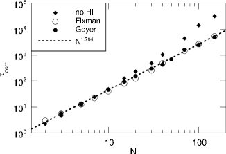
Figure 3: Relaxation times $\tau_{corr}$ of the autocorrelation function of the end-to-end vector $\vec{R}_{ee}$ of polymers of various lengths $N$ from BD simulations without HI (diamonds) and with HI according to Fixman’s Chebyshev approximation (open points) and our truncated expansion approximation (filled points), respectively. The relaxation times were obtained by fitting a stretched exponential to the autocorrelation function. The dashed line indicates the scaling $\propto N^{3\nu}$ with $\nu=0.588$.

Another measure, which is sensitive to the internal dynamics of the polymer, is the autocorrelation function $\langle\vec{R}_{ee}(t)\cdot\vec{R}_{ee}(0)\rangle$ of the end-to-end vector $\vec{R}_{ee}$, which decays exponentially with a time constant $\tau_{corr}$ (the Zimm time). Figure 3 shows that the fitted relaxation times are proportional to $N^{3\nu}$ as predicted theoretically. With our TEA-HI, the relaxation is again slightly slower by some 10%, which indicates that our approximation takes most of the hydrodynamic correlation between the beads into account. Without HI, the relaxation of $\vec{R}_{ee}$ takes about one order of magnitude longer at $N=100$ and even more for longer chains.

III.5 Runtime considerations

Without HI, one needs to evaluate at each timestep the forces from the $N-1$ springs connecting the $N$ beads and also the $N(N-1)/2$ repulsive two-body interactions. For each of the $N$ beads a random displacement has to be chosen and then the beads are moved according to the external and the random forces. Consequently, the observed runtime $T$ per timestep can be fitted with $T=t_{0}+t_{1}\,N+t_{2}\,N(N-1)$ as shown in figure 4. For one million timesteps on a 2.8 GHz Pentium 4 CPU, we obtained $t_{0}=0.2$ seconds, $t_{1}=0.95$ seconds, and $t_{2}=0.038$ seconds. To obtain the runtimes, we ran each of the simulations for several minutes until the runtime for one million timesteps could be calculated with sufficient statistical accuracy.

With HI, also the hydrodynamic tensor has to be set up, for which $N(N-1)/2$ distances between the beads have to be calculated. For our truncated expansion, the $N$ normalization constants $C_{i}$ (20) are evaluated in $\mathcal{O}(N^{2})$ time. For the expansion coefficients $\beta_{ij}$, the average coupling $\epsilon=\langle D_{ij}/D_{ii}\rangle$ is required, for which the $(N-1)(N-2)/2$ off-diagonal entries of the diffusion tensor have to be summed up. Finally, the effective hydrodynamically corrected forces of equations (15) and (16) are evaluated in $\mathcal{O}(N^{2})$ time, leading to an overall quadratic runtime that can be fitted with $t_{0}=1$ seconds, $t_{1}=0.2$ seconds, and $t_{2}=0.3$ seconds for one million timesteps. For the very simple polymer model used, the inclusion of HI thus slowed down the simulations by a constant factor of about ten for large $N$. For more realistic —and thus more expensive—interactions between the individual beads, the relative cost of considering HI will even decrease.

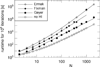
Figure 4: Comparison of the runtime behavior of BD simulations with the different methods to include HI vs. the chain length $N$ of the bead-spring polymer. The datapoints give the times required to simulate one million timesteps, the lines are polynomial fits to the data as explained in the text.

In the original formulation of Ermak and McCammon ERM78 , the random displacements are determined via a Cholesky factorization of the diffusion tensor. This led to the expected runtime behavior of $\mathcal{O}(N^{3})$ in our simulations, which was fitted with $T=0.027N^{3}+1.5N^{2}+0.8N$ seconds for one million timesteps (see figure 4). The more efficient Chebyshev expansion led to an effective runtime of $\mathcal{O}(N{{}^{2.5}})$, i.e., $T=0.14N^{2.5}+4N$ at an accuracy of $\epsilon_{f}=10^{-3}$. Reducing $\epsilon_{f}$ to $10^{-2}$ or $10^{-1}$ led to a small speedup of a factor of 2 or 3, respectively. We note that the Chebyshev expansion needs a lot of computer memory for the repeated matrix-vector multiplications, especially for large particle numbers. Consequently, at $N=1000$ the Chebyshev approximation was slowed down due to memory constraints of the computer we used and the runtime for $N=2000$ could not be determined any more on this machine. For our approximation, the memory requirements were determined by the diffusion tensor, while the Cholesky factorization needed additional temporary storage of about the same size as the diffusion tensor.

With the very simple interactions between the beads that we used here in the simulations, the inclusion of hydrodynamics with our approximation slowed down the simulation by a constant factor of about ten. A simulation of a polymer of 1000 beads would consequently run for about half of a day with our approximated HI for every hour it takes without HI. The same simulation would take four to five days with Fixman’s Chebyshev approximation and more than a month with the original algorithm of Ermak and McCammon.

The propagation was performed with the simple Euler propagator and a rather conservative timestep. The simulations therefore could be easily accelerated by using a more advanced propagation scheme like, e.g., the semiimplicit scheme of Jendrejack JEN00 or the Trotter expansion of De Fabritiis et al. FAB06 .

As our approximation calculates the effective random forces from individual two-body contributions, it is now also possible to introduce distance dependent cut-offs to the hydrodynamic interactions to reduce the number of terms that have to be summed up. Similar to the cut-offs for direct interactions, this will speed up the simulation. With the traditional methods of Ermak and McCammon or of Fixman, a cut-off would lead to vanishing entries in the diffusion tensor without reducing its size and, thus, the numerical effort to factorize it. With these algorithms, cut-offs only introduce errors in the dynamics without any gain. We did not consider cut-offs here, as it is a project on its own to investigate the trade-off between the perturbations of the hydrodynamic interactions vs. the achieved runtime savings.

Finally, we note that with the two-body contributions used in our TEA-HI, the hydrodynamic coupling can be summed up in parallel to the inter-particle forces. Then, there is no need to build up and keep the complete $3N\times 3N$ hydrodynamic tensor in computer memory, only the actually required $3\times 3$ submatrices $\mathbf{D}_{ij}$ of equations (5) and (7) have to be determined temporarily. Then the required memory for many-particle simulations increases only linearly with $N$. Consequently, our truncated expansion is not only faster than the originally proposed Cholesky factorization and the improved Chebyshev expansion, but it also needs much less computer memory, which allows for even larger systems to be handled efficiently.

IV Conclusions

We showed how the correlated random displacements can be approximated efficiently in Brownian dynamics simulations with hydrodynamic interactions. In our truncated expansion approximation, effective hydrodynamically corrected random forces are determined with the aim to reproduce the statistical moments of the thermal motion. Truncating the expansion at the second order allows to calculate the random forces from individual two-body contributions in $\mathcal{O}(N^{2})$ time. For these only $3\times 3$ submatrices of the $3N\times 3N$ hydrodynamic tensor are required temporarily. Our approximation consequently has the same runtime and storage scaling as the calculation of the direct interactions between the particles.

We then compared the simulation results with our approximation to the results obtained with the exact method of Ermak and McCammon and with the Chebyshev approximation of Fixman, the runtimes of which scaled as $\mathcal{O}(N^{3})$ and $\mathcal{O}(N^{2.5})$, respectively.

Both the dynamics of a bead-spring dimer with variable separation of the beads and of polymers of chain lengths of $N=2\ldots 200$ showed that our approximation captures about 95% of the hydrodynamically introduced correlation. For most applications on chemical or biological systems, where the direct interactions have to be approximated anyway, this appears a completely sufficient level of accuracy. Moreover, it allows for accounting of important hydrodynamic effects in systems where they were sofar mostly ignored for computational reasons.

As already mentioned above, we see the main application of our truncated expansion hydrodynamics in Brownian dynamics simulations of large biological systems, where one is interested in the dynamics of many-particle association GOR04 , transport processes, or protein folding where the complicated interactions between the proteins or parts thereof have to be approximated rather crudely. For these applications, it is surely better to include most of the effects of hydrodynamics without slowing down the simulation too much than to either have no HI at all or the correct HI at a prohibitive computational cost. Other applications could be to describe the behavior of non-spherical particles by assembling them from smaller spheres DIC84 ; GAR81 . Here the quality of the model increases with the number of spheres used to build the non-spherical particles.

References

- (1) R. R. Gabdoulline and R. C. Wade, Curr. Op. Struc. Biol. 12, 204 (2002)
- (2) E. L. Gross and D. C. Pearson, Biophys. J. 85, 2055 (2003)
- (3) C. Gorba, T. Geyer, and V. Helms, J. Chem. Phys. 121, 457 (2004)
- (4) A. Spaar, C. Dammer, R. R. Gabdoulline, R. C. Wade, and V. Helms, Biophys. J. 90, 1913 (2006)
- (5) J. P. Hernández-Ortiz, H. Ma, J. J. de Pablo, and M. D. Graham, Phys. Fluids 18, 123101 (2006)
- (6) M. Dlugosz, J. A. Antosiewicz, and J. Trylska, J. Chem. Theory Comput. 4, 549 (2007)
- (7) A. Einstein, Ann. d. Physik 17, 549 (1905)
- (8) J. K. G. Dhont, An Introduction to Dynamics of Colloids (Elsevier, Amsterdam, 1996)
- (9) J. M. Deutch and I. Oppenheim, J. Chem. Phys. 54, 3547 (1971)
- (10) D. L. Ermak and J. A. McCammon, J. Chem. Phys. 69, 1352 (1978)
- (11) S. R. McGuffee and A. H. Elcock, J. Am. Chem. Soc. 128, 12098 (2006)
- (12) P. Ahlrichs, R. Everaers, and B. Dünweg, Phys. Rev. E 64, 040501(R) (2001)
- (13) T. Zhou and S. B. Chen, J. Chem. Phys. 124, 034904 (2006)
- (14) P. Szymczak and M. Cieplak, J. Chem. Phys. 127, 155106 (2007)
- (15) M. Fixman, Macromol. 19, 1204 (1986)
- (16) D. M. Heyes, J. Phys.: Condens. Matter 7, 8857 (1995)
- (17) A. J. Banchio and J. F. Brady, J. Chem. Phys. 118, 10323 (2003)
- (18) J. Huang and T. Schlick, J. Chem. Phys. 117, 8573 (2002)
- (19) E. Dickinson, S. A. Allison, and J. A. McCammon, J. Chem. Soc., Faraday Trans. 2 81, 591 (1984)
- (20) J. G. Kirkwood and J. Riseman, J. Chem. Phys. 16, 565 (1948)
- (21) J. Rotne and S. Prager, J. Chem. Phys. 50, 4831 (1969)
- (22) H. Yamakawa, J. Chem. Phys. 53, 436 (1970)
- (23) J. Garcia de la Torre and V. A. Bloomfield, Biopolymers 16, 1747 (1977)
- (24) W. H. Press, S. A. Teukolsky, W. T. Vetterling, and B. P. Flannery, Numerical Recipes in Fortran 77, Vol. 1, (Cambridge University Press, Cambridge, 1997)
- (25) R. M. Jendrejack, M. D. Graham, and J. J. de Pablo, J. Chem. Phys. 113, 2894 (2000)
- (26) M. Galassi, J. Davies, J. Theiler, B. Gough, G. Jungman, M. Booth, and F. Rossi, GNU Scientific Library Reference Manual, 2nd Ed., (Network Theory Ltd., Bristol, 2006)
- (27) B. Li, N. Madras, and A. D. Sokal, J. Stat. Phys. 80, 661 (1995)
- (28) B. Dünweg, D. Reith, M. Steinhauser, and K. Kremer, J. Chem. Phys. 2002, 914 (2002)
- (29) B. Liu and B. Dünweg, J. Chem. Phys. 118, 8061 (2003)
- (30) G. De Fabritiis, M. Serrano, P. Español, and P. V. Coveney, Physica A 361, 429 (2006)
- (31) J. Garcia de la Torre and V. A. Bloomfield, Q. Rev. Biophys. 14, 81 (1981)