Einstein–Podolsky–Rosen correlations of vector bosons

Abstract

We calculate the joint probabilities and the correlation function in Einstein–Podolsky–Rosen type experiments with a massive vector boson in the framework of quantum field theory. We report on the strange behavior of the correlation function (and the probabilities) – the correlation function, which in the relativistic case still depends on the particle momenta, for some fixed configurations has local extrema. We also show that relativistic spin-1 particles violate some Bell inequalities more than nonrelativistic ones and that the degree of violation of the Bell inequality is momentum dependent.

I Introduction

Different aspects of quantum information theory Nielsen and Chuang (2000) in the relativistic context have been discussed in many papers Ahn et al. (2002, 2003a, 2003b); Alsing and Milburn (2002); Bartlett and Terno (2005); Caban and Rembieliński (2003, 2005, 2006); Czachor and Wilczewski (2003); Czachor (1997a, b, 2005); Gingrich and Adami (2002); Gingrich et al. (2003); Gonera et al. (2004); Harshman (2005); He et al. (2007a, b); Jordan et al. (2005, 2006); Kosiński and Maślanka (2003); Kim and Son (2005); Li and Du (2003, 2004); Lamata et al. (2006); Lindner et al. (2003); Lee and Chang-Young (2004); Moon et al. (2003); Pachos and Solano (2003); Peres et al. (2002, 2005); Peres and Terno (2003a, b, 2004); Rembieliński and Smoliński (2002); Soo and Lin (2004); Terno (2003, 2005); Terashima and Ueda (2003a, b); You et al. (2004); Zbinden et al. (2001), mostly for massive particles. Photons have only been discussed in a few papers Alsing and Milburn (2002); Bartlett and Terno (2005); Caban and Rembieliński (2003); Gingrich et al. (2003); Lindner et al. (2003); Peres and Terno (2003a, b, 2004); Terno (2005); Terashima and Ueda (2003a). Most of these works were performed in the framework of relativistic quantum mechanics. However, for the discussion of relativistic covariance the most appropriate framework is the quantum field theory (QFT) approach. Recently we have discussed the Einstein–Podolsky–Rosen (EPR) correlation function for a pair of spin-$\tfrac{1}{2}$ massive particles in the QFT framework Caban and Rembieliński (2006). In the present paper we consider a pair of spin-1 massive particles in this framework and calculate the correlation function in EPR-type experiments for such a pair in a covariant scalar state. We also calculate the probabilities of the definite outcomes of spin projections measurements performed by two observers – Alice and Bob.

We observe very surprising behavior of the correlation function (as well as the probabilities). In the center-of-mass frame for the definite configuration of the particles momenta and directions of the spin projection measurements the correlation function still depends on the value of the particle momentum. It also appears that for some configurations this dependence is not monotonic. In other words, for fixed spin measurement directions and particle momenta directions, the correlation function (and probabilities) can have an extremum for some finite value of the particle momentum. As far as we are aware this is the first time, that such behavior of the correlation function has been reported.

This strange behavior of the correlation function also affects the violation of the Bell-type inequalities. Our analysis shows that relativistic vector bosons violate Bell inequalities stronger than nonrelativistic spin-1 particles and that the degree of violation of Bell inequality depends on the particle momentum.

In Sec. II we establish notation and recall basic facts concerning the massive spin-1 representation of the Poincaré group and quantum spin-1 boson field. In Sec. III we define one- and two-particle states which transform covariantly with respect to the Lorentz group. In the next section we discuss the spin operator. Sec. V is devoted to the explicit calculation of the probabilities and correlation function for the boson pair in the scalar state. In Sec. VI we discuss our correlation function and probabilities . Sec. VII is devoted to the analysis of Bell-type inequalities for spin 1 particles in the relativistic context. The last section contains our concluding remarks.

In the paper we use the natural units $\hbar=c=1$ and the metric tensor $\eta^{\mu\nu}=\textrm{diag}(1,-1,-1,-1)$.

II Preliminaries

For the readers convenience we recall the basic facts and formulas concerning the spin one representation of the Poincaré group and quantum vector boson field.

II.1 Massive representations of the Poincaré group

Let us denote by $\mathcal{H}$ the carrier space of the irreducible massive representation of the Poincaré group. It is spanned by the four-momentum operator eigenvectors $|k,\sigma\rangle$

$$\hat{P}^{\mu}|k,\sigma\rangle=k^{\mu}|k,\sigma\rangle,$$ (1)

$k^{2}=m^{2}$, with $m$ denoting the mass of the particle, and $\sigma$ its spin component along z axis. We use the following Lorentz-covariant normalization

$$\langle k,\sigma|k^{\prime},\sigma^{\prime}\rangle=2k^{0}\delta^{3}(\textbf{k}-\textbf{k}^{\prime})\delta_{\sigma\sigma^{\prime}}.$$ (2)

The vectors $|k,\sigma\rangle$ can be generated from standard vector $|\tilde{k},\sigma\rangle$, where $\tilde{k}=m(1,0,0,0)$ is the four-momentum of the particle in its rest frame. We have $|k,\sigma\rangle=U(L_{k})|\tilde{k},\sigma\rangle$, where Lorentz boost $L_{k}$ is defined by relations $k=L_{k}\tilde{k}$, $L_{\tilde{k}}=\operatorname{\openone}$. The explicit form of $L_{k}$ is

$$L_{k}=\left(\begin{array}[]{c|c}\tfrac{k^{0}}{m}&\tfrac{\mathbb{k}^{T}}{m}\\ \hline\cr\tfrac{\mathbb{k}}{m}&\operatorname{\openone}+\tfrac{\mathbb{k}\otimes\mathbb{k}^{T}}{m(m+k^{0})}\end{array}\right),$$ (3)

where $k^{0}=\sqrt{m^{2}+\mathbb{k}^{2}}$.

By means of Wigner procedure we get

$$U(\Lambda)|k,\sigma\rangle=\mathcal{D}^{s}_{\lambda\sigma}(R(\Lambda,k))|\Lambda k,\lambda\rangle,$$ (4)

where the Wigner rotation $R(\Lambda,k)$ is defined as $R(\Lambda,k)=L_{\Lambda k}^{-1}\Lambda L_{k}$. Because we are going to analyze correlations of spin one particles, in the sequel we will focus on the representation $\mathcal{D}^{1}(R(\Lambda,k))\equiv\mathcal{D}(R)$. There exists such unitary matrix $V$ that every matrix $\mathcal{D}(R)$ is related to $R$ by

$$\mathcal{D}(R)=VRV^{{\dagger}}.$$ (5)

$\mathcal{D}(R)$ are generated by $\mathbb{S}^{i}$, $i=1,2,3$,

$$S^{1}=\tfrac{1}{\sqrt{2}}\left(\begin{array}[]{ccc}0&1&0\\ 1&0&1\\ 0&1&0\\ \end{array}\right),\;S^{2}=\tfrac{i}{\sqrt{2}}\left(\begin{array}[]{ccc}0&-1&0\\ 1&0&-1\\ 0&1&0\\ \end{array}\right),$$ (12)

$$\,\,\,\,\,S^{3}=\left(\begin{array}[]{ccc}1&0&0\\ 0&0&0\\ 0&0&-1\\ \end{array}\right),$$ (16)

(see e.g. Messiah (1962)), that is $\mathcal{D}(R)=e^{i\boldsymbol{\phi}\mathbb{S}}$. Taking into account the form of generators of the rotations $R$ i.e. $[I^{i}]_{jk}=-i\epsilon_{ijk}$, we can easily determine the explicit form of matrix V

$$V=\frac{1}{\sqrt{2}}\left(\begin{array}[]{ccc}-1&i&0\\ 0&0&\sqrt{2}\\ 1&i&0\\ \end{array}\right).$$ (17)

II.2 Vector field

Under Lorentz group action the vector boson field operator $\hat{\varphi}^{\mu}(x)$ transforms according to

$$U(\Lambda)\hat{\varphi}^{\mu}(x)U^{{\dagger}}(\Lambda)=(\Lambda^{-1})^{\mu}_{\,\,\nu}\hat{\varphi}^{\nu}(\Lambda x).$$ (18)

The field operator has the standard momentum expansion

$$\hat{\varphi}^{\mu}(x)=(2\pi)^{-3/2}\sum_{\sigma=0,\pm 1}\int d\mu(k)\left[e^{ikx}e^{\mu}_{\,\,\sigma}(k)a_{\sigma}^{{\dagger}}(k)\right.$$

$$\left.+e^{-ikx}e^{*\mu}_{\,\,\,\,\,\sigma}(k)a_{\sigma}(k)\right],$$ (19)

where $d\mu(k)=\Theta(k^{0})\delta((k^{0})^{2}-\omega_{k}^{2})\equiv\frac{d^{3}\textbf{k}}{2\omega_{k}}$ is the Lorentz-invariant measure, $\omega_{k}=\sqrt{\mathbb{k}^{2}+m^{2}}$, $a_{\sigma}^{{\dagger}}(k)$ and $a_{\sigma}(k)$ are creation and annihilation operators of the particle with four-momentum $k$ and spin component along z-axis equal to $\sigma$. They fulfill canonical commutation relations

$$[a_{\sigma}^{{\dagger}}(k),a_{\sigma^{\prime}}^{{\dagger}}(k^{\prime})] = [a_{\sigma}(k),a_{\sigma^{\prime}}(k^{\prime})]=0,$$ (20a)

$$[a_{\sigma}(k),a^{{\dagger}}_{\sigma^{\prime}}(k^{\prime})] = 2k^{0}\delta(\textbf{k}-\textbf{k}^{\prime})\delta_{\sigma\sigma^{\prime}}.$$ (20b)

The field satisfies Klein-Gordon equation and Lorentz transversality condition, which imply

$$m^{2}=k^{2},\quad k_{\mu}e^{\mu}_{\,\,\sigma}(k)=0.$$ (21)

The one-particle states $|k,\sigma\rangle:=a_{\sigma}^{{\dagger}}(k)|0\rangle$ transform according to (4) provided that

$$U(\Lambda)a_{\sigma}^{{\dagger}}(k)U^{{\dagger}}(\Lambda) = \mathcal{D}_{\lambda\sigma}(R(\Lambda,k))a_{\lambda}^{{\dagger}}(\Lambda k),$$ (22a)

$$U(\Lambda)a_{\sigma}(k)U^{{\dagger}}(\Lambda) = \mathcal{D}^{*}_{\lambda\sigma}(R(\Lambda,k))a_{\lambda}(\Lambda k).$$ (22b)

Here $|0\rangle$ denotes Poincaré invariant vacuum with $\langle 0|0\rangle=1$; $a_{\sigma}(k)|0\rangle=0$. Equations (18,22) imply the Weinberg conditions for amplitudes $e^{\mu}_{\,\,\sigma}(k)$

$$e^{\mu}_{\,\,\sigma}(\Lambda k)=\Lambda^{\mu}_{\,\,\nu}e^{\nu}_{\,\,\lambda}(k)\mathcal{D}(R(\Lambda,k))_{\sigma\lambda}.$$ (23)

From Eq. (23) we have

$$e(k)=L_{k}e(\tilde{k}),$$ (24)

where $L_{k}$ is given by (3) and we used the fact that $R(L_{k},\tilde{k})=\operatorname{\openone}$. Therefore, to find the explicit form of $e^{\mu}_{\,\,\sigma}(k)$ it is enough to determine $e^{\mu}_{\,\,\sigma}(\tilde{k})$. From Eq. (21) we get

$$[e^{\mu}_{\,\,\sigma}(\tilde{k})]=\left(\begin{array}[]{ccc}0&0&0\\ \hline\cr&\tilde{e}&\\ \end{array}\right),$$ (25)

where $\tilde{e}$ is a $3\times 3$ matrix. Now, from the Weinberg condition (23) for pure rotations and by means of Eq. (5) and Schur’s Lemma we find

$$\tilde{e}=V^{\mathrm{T}},$$ (26)

where explicit form of $V$ is given by (17). Finally from (24) we have

$$e(k)=\left(\begin{array}[]{c}\tfrac{\mathbb{k}^{T}}{m}\\ \hline\cr\operatorname{\openone}+\tfrac{\mathbb{k}\otimes\mathbb{k}^{T}}{m(m+k^{0})}\end{array}\right)V^{\mathrm{T}}.$$ (27)

Equations (26,27) imply

$$e^{*\mu}_{\,\,\,\,\,\sigma}(k)e_{\mu\lambda}(k)=-\delta_{\sigma\lambda},$$ (28a)

$$e^{\mu}_{\,\,\sigma}(k)e_{\mu\lambda}(k)=-(VV^{\mathrm{T}})_{\sigma\lambda},$$ (28b)

$$e^{*\mu}_{\,\,\,\,\,\sigma}(k)e^{\nu}_{\,\,\sigma}(k)=-\eta^{\mu\nu}+\tfrac{k^{\mu}k^{\nu}}{m^{2}},$$ (28c)

where $e(k)VV^{\mathrm{T}}=e^{*}(k)$, and $VV^{\mathrm{T}}=\left(\begin{array}[]{ccc}0&0&-1\\ 0&1&0\\ -1&0&0\\ \end{array}\right)$.

III Covariant states

III.1 One-particle covariant states

In the discussion of Lorentz-covariance it is convenient to use states

$$|(\mu,k)\rangle=e^{\mu}_{\,\,\sigma}(k)|k,\sigma\rangle,$$ (29)

which transform covariantly

$$U(\Lambda)|(\mu,k)\rangle=(\Lambda^{-1})^{\mu}_{\,\,\nu}|(\nu,\Lambda k)\rangle.$$ (30)

They are normalized as follows [c.f. (2)]

$$\langle(\mu,k)|(\nu,p)\rangle=2k^{0}\delta(\mathbb{k}-\mathbb{p})e^{*\mu}_{\,\,\,\sigma}(k)e^{\nu}_{\,\,\sigma}(p).$$ (31)

Arbitrary one-particle state can be expanded in the standard basis $|k,\sigma\rangle$ as well as in the covariant one (29)

$$|\psi\rangle=\int d\mu(k)\psi_{\sigma}(k)|k,\sigma\rangle=\int d\mu(k)\Psi_{\mu}(k)|(\mu,k)\rangle,$$ (32)

where

$$\Psi_{\mu}(k)e^{\mu}_{\,\,\sigma}(k)=\psi_{\sigma}(k).$$ (33)

III.2 Two-particle covariant states

In analogy to (29) we can define covariant basis in the two-particle sector of the Fock space

$$|(\mu,k),(\nu,p)\rangle=e^{\mu}_{\,\,\sigma}(k)e^{\nu}_{\,\,\lambda}(p)|(k,\sigma),(p,\lambda)\rangle,$$ (34)

where $|(k,\sigma),(p,\lambda)\rangle=a^{{\dagger}}_{\,\sigma}(k)a^{{\dagger}}_{\,\lambda}(p)|0\rangle$. The most general two-particle state has the form

$$|\Psi\rangle=\int d\mu(k)d\mu(p)\psi_{\sigma\lambda}(k,p)|(k,\sigma),(p,\lambda)\rangle\\ \equiv\int d\mu(k)d\mu(p)\Psi_{\mu\nu}(k,p)|(\mu,k),(\nu,p)\rangle.$$ (35)

One can see that

$$\Psi_{\mu\nu}(k,p)e^{\mu}_{\,\,\sigma}(k)e^{\nu}_{\,\,\lambda}(p)=\psi_{\sigma\lambda}(k,p).$$ (36)

Moreover it holds

$$\Psi^{\mu\nu}(k,p)=\Psi^{\nu\mu}(p,k),$$ (37a)

$$k_{\mu}\Psi^{\mu\nu}(k,p)=\Psi^{\mu\nu}(k,p)p_{\nu}=0.$$ (37b)

We can now define two-particle states transforming according to irreducible representations of Lorentz group. The scalar state describing particles with sharp momenta is defined as

$$|\Psi_{s}\rangle=\eta_{\mu\nu}|(\mu,k),(\nu,p)\rangle.$$ (38)

In terms of (34) it takes the form

$$|\Psi_{s}\rangle=\eta_{\mu\nu}e^{\mu}_{\,\,\sigma}(k)e^{\nu}_{\,\,\lambda}(p)|(k\sigma),(p,\lambda)\rangle.$$ (39)

There are also two independent tensor states, the symmetric traceless

$$|\Psi_{sym}^{\mu\nu}\rangle=\tfrac{1}{2}(\delta^{\mu}_{\,\,\alpha}\delta^{\nu}_{\,\,\beta}+\delta^{\mu}_{\,\,\beta}\delta^{\nu}_{\,\,\alpha}-\tfrac{1}{2}\eta^{\mu\nu}\eta_{\alpha\beta})|(\alpha,k),(\beta,p)\rangle,$$ (40)

and the antisymmetric one

$$|\Psi_{asym}^{\mu\nu}\rangle=\tfrac{1}{2}(\delta^{\mu}_{\,\,\alpha}\delta^{\nu}_{\,\,\beta}-\delta^{\mu}_{\,\,\beta}\delta^{\nu}_{\,\,\alpha})|(\alpha,k),(\beta,p)\rangle.$$ (41)

In the sequel we will analyze correlations in the scalar state (38).

IV Spin operator

When we want to calculate explicitly correlation functions, we need to introduce the spin operator for relativistic massive particles. Several possibilities have been discussed in the literature (see e.g. Czachor (1997a); Czachor and Wilczewski (2003); Terno (2003); Rembieliński and Smoliński (2002); Caban and Rembieliński (2005, 2006); Lee and Chang-Young (2004); Li and Du (2003); Soo and Lin (2004); Terashima and Ueda (2003a, b)). We choose the operator

$$\hat{\mathbb{S}}=\frac{1}{m}\left(\hat{\mathbb{W}}+\hat{W}^{0}\frac{\mathbb{\hat{P}}}{\hat{P}^{0}+m}\right),$$ (42)

which is the most appropriate Terno (2003); Caban and Rembieliński (2005); Bogolubov et al. (1975). Here

$$\hat{W}^{\mu}=\tfrac{1}{2}\epsilon^{\mu\nu\gamma\delta}\hat{P}_{\nu}\hat{J}_{\gamma\delta}$$ (43)

is the Pauli-Lubanski four-vector, $\hat{P}_{\nu}$ is the four-momentum operator, $\hat{J}_{\mu\nu}$ denote the generators of the Lorentz group such that $U(\Lambda)=\exp(i\omega^{\mu\nu}\hat{J}_{\mu\nu})$, and we assume $\epsilon^{0123}=1$. Consequently the spin operator $\hat{\mathbb{S}}$ acts on one-particle states according to

$$\hat{\mathbb{S}}|k,\sigma\rangle=\mathbb{S}_{\lambda\sigma}|k,\lambda\rangle,$$ (44)

where $S^{i}$ are defined by (12). In the Fock space $\hat{\mathbb{S}}$ takes standard form

$$\hat{\mathbb{S}}=\int d\mu(k)a^{{\dagger}}(k)\mathbb{S}a(k),$$ (45)

where the column matrix $a(k)\nolinebreak=\nolinebreak\left(a_{+1}(k),a_{0}(k),a_{-1}(k)\right)^{\mathrm{T}}$. From Eqs. (28a,29) we get

$$\mathbb{\hat{S}}|(\alpha,k)\rangle=-\big{[}e(k)\mathbb{S}^{T}e^{{\dagger}}(k)\eta\big{]}^{\alpha}_{\phantom{\alpha}\beta}|(\beta,k)\rangle.$$ (46)

In real experiments detectors register only particles whose momenta belong to some definite region $\Omega$ in momentum space. Therefore we need the operator which acts similar to (44) on particles with four-momenta belonging to $\Omega$ and yields $0$ in all other cases. Such an operator has the following form

$$\hat{\mathbb{S}}_{\Omega}=\int_{\Omega}d\mu(k)a^{{\dagger}}(k)\mathbb{S}a(k).$$ (47)

V Probabilities and the correlation function

Let us consider two distant observers, Alice and Bob, in the same inertial frame, sharing a pair of bosons in scalar state $|\Psi_{s}\rangle$ defined by (39).

Now let Alice measure spin component of her boson in direction $\mathbb{a}$ and Bob spin component of his boson in direction $\mathbb{b}$, where $|\mathbb{a}|=|\mathbb{b}|=1$. Their observables are $(\mathbb{a}\cdot\mathbb{\hat{S}}_{A})$ and $(\mathbb{b}\cdot\mathbb{\hat{S}}_{B})$, respectively, where $(\boldsymbol{\omega}\cdot\hat{\mathbb{S}}_{\Omega})$ is defined by (47) with $\Omega$ equal $A$ and $B$, and $\boldsymbol{\omega}$ equal to a and b, respectively. We assume that $A\cap B=\emptyset$. Now we would like to explicitly calculate probabilities $P_{\sigma\lambda}$ of obtaining particular outcomes $\sigma$ and $\lambda$ by Alice and Bob, respectively ($\sigma$ and $\lambda$ can take values $\pm 1$ and $0$). Let us first notice, that from Eqs. (34), (44), and (47) we have

$$(\boldsymbol{\omega}\cdot\hat{\mathbb{S}}_{\Omega})|(k,\lambda),(p,\sigma)\rangle\\ =\boldsymbol{\omega}\cdot\big{[}\chi_{\Omega}(k)\mathbb{S}_{\lambda^{\prime}\lambda}\delta_{\sigma^{\prime}\sigma}+\chi_{\Omega}(p)\mathbb{S}_{\sigma^{\prime}\sigma}\delta_{\lambda^{\prime}\lambda}\big{]}|(k,\lambda^{\prime}),(p,\sigma^{\prime})\rangle,$$ (48)

where the characteristic function $\chi_{\Omega}(q)$ is defined in a standard way

$$\chi_{\Omega}(q)=\left\{\begin{array}[]{ccccc}1&&&&\text{when}\,\,q\in\Omega,\\ 0&&&&\text{when}\,\,q\notin\Omega.\\ \end{array}\right.$$ (49)

However, in EPR-type experiments we take into account only such measurements in which Alice and Bob register one particle each. Therefore we are actually interested in spectral decomposition of observable $(\boldsymbol{\omega}\cdot\hat{\mathbb{S}}_{\Omega})\hat{\Pi}^{1}_{\Omega}$, where $\hat{\Pi}^{1}_{\Omega}$ is a projector (in the two-particle sector of the Fock space) on the subspace of states corresponding to the situation in which exactly one particle has momentum from the region $\Omega$. To find the explicit form of the $\hat{\Pi}^{1}_{\Omega}$ we use the particle number operator $\hat{N}_{\Omega}$ answering the question how many particles have momentum from $\Omega$. In the two-particle sector of the Fock space we have the obvious spectral decomposition of $\hat{N}_{\Omega}$

$$\hat{N}_{\Omega}=0\cdot\hat{\Pi}^{0}_{\Omega}+1\cdot\hat{\Pi}^{1}_{\Omega}+2\cdot\hat{\Pi}^{2}_{\Omega},$$ (50)

and in the basis (34)

$$\hat{N}_{\Omega}|(k,\lambda),(p,\sigma)\rangle=\big{[}\chi_{\Omega}(k)+\chi_{\Omega}(p)\big{]}|(k,\lambda),(p,\sigma)\rangle.$$ (51)

In Eq. (50) $\hat{\Pi}_{\Omega}^{i}$, $i=0,1,2$, denotes a projector on the subspace of two-particle states, in which exactly $i$ particles have momenta from $\Omega$. From Eqs. (50, 51) we find

$$\hat{\Pi}_{\Omega}^{1}=2\hat{N}_{\Omega}-\hat{N}_{\Omega}^{2},$$ (52)

and

$$\hat{\Pi}_{\Omega}^{1}|(k,\lambda),(p,\sigma)\rangle\\ =\big{[}\chi_{\Omega}(k)+\chi_{\Omega}(p)-2\chi_{\Omega}(k)\chi_{\Omega}(p)\big{]}|(k,\lambda),(p,\sigma)\rangle.$$ (53)

Therefore from (48) and (53) we finally get

$$(\boldsymbol{\omega}\cdot\hat{\mathbb{S}}_{\Omega})\Pi^{1}_{\Omega}|(k,\lambda),(p,\sigma)\rangle\\ =\boldsymbol{\omega}\cdot\Big{\{}\chi_{\Omega}(k)\big{[}1-\chi_{\Omega}(p)\big{]}\mathbb{S}_{\lambda^{\prime}\lambda}\delta_{\sigma^{\prime}\sigma}\\ +\chi_{\Omega}(p)\big{[}1-\chi_{\Omega}(k)\big{]}\mathbb{S}_{\sigma^{\prime}\sigma}\delta_{\lambda^{\prime}\lambda}\Big{\}}|(k,\lambda^{\prime}),(p,\sigma^{\prime})\rangle.$$ (54)

By definition the observable $\boldsymbol{\omega}\hat{\mathbb{S}}_{\Omega}\hat{\Pi}^{1}_{\Omega}$ measures the spin component of one particle in the direction $\boldsymbol{\omega}$, therefore its spectral decomposition is

$$(\boldsymbol{\omega}\cdot\hat{\mathbb{S}}_{\Omega})\hat{\Pi}^{1}_{\Omega}=1\cdot\hat{\Pi}^{+}_{\Omega\boldsymbol{\omega}}-1\cdot\hat{\Pi}^{-}_{\Omega\boldsymbol{\omega}}+0\cdot\hat{\Pi}^{0}_{\Omega\boldsymbol{\omega}},$$ (55)

where the projectors $\hat{\Pi}^{\pm}_{\Omega\boldsymbol{\omega}}$ and $\hat{\Pi}^{0}_{\Omega\boldsymbol{\omega}}$ correspond to eigenvalues $\pm 1$ and $0$, respectively. Simple calculation gives

$$\hat{\Pi}^{\pm}_{\Omega\boldsymbol{\omega}} = \tfrac{1}{2}(\boldsymbol{\omega}\cdot\hat{\mathbb{S}}_{\Omega})\big{[}(\boldsymbol{\omega}\cdot\hat{\mathbb{S}}_{\Omega})\pm\operatorname{\openone}\big{]}\hat{\Pi}_{\Omega}^{1},$$ (56a)

$$\hat{\Pi}^{0}_{\Omega\boldsymbol{\omega}} = \big{[}\operatorname{\openone}-(\boldsymbol{\omega}\cdot\hat{\mathbb{S}}_{\Omega})^{2}\big{]}\hat{\Pi}_{\Omega}^{1}.$$ (56b)

Now we can find explicitly the probabilities $P_{\sigma\lambda}$ mentioned above in the state (39).

$$P_{\sigma\lambda} = \frac{\langle\Psi_{s}|\hat{\Pi}_{A\mathbb{a}}^{\sigma}\hat{\Pi}_{B\mathbb{b}}^{\lambda}|\Psi_{s}\rangle}{\langle\Psi_{s}|\Psi_{s}\rangle}.$$ (57)

From Eqs. (48, 53, 54, 56) we find

$$\hat{\Pi}^{\pm}_{\Omega\boldsymbol{\omega}}|\Psi_{s}\rangle=\tfrac{1}{2}\eta_{\mu\nu}e^{\mu}_{\phantom{\mu}\lambda}(k)e^{\nu}_{\phantom{\nu}\sigma}(p)\Big{\{}\big{[}(\boldsymbol{\omega}\cdot\textbf{S})^{2}\pm\boldsymbol{\omega}\cdot\textbf{S}\big{]}_{\lambda^{\prime}\lambda}\delta_{\sigma^{\prime}\sigma}\chi_{\Omega}(k)\big{[}1-\chi_{\Omega}(p)\big{]}\\ +\big{[}(\boldsymbol{\omega}\cdot\textbf{S})^{2}\pm\boldsymbol{\omega}\cdot\textbf{S}\big{]}_{\delta^{\prime}\delta}\delta_{\lambda^{\prime}\lambda}\chi_{\Omega}(p)\big{[}1-\chi_{\Omega}(k)\big{]}\Big{\}}|(k,\lambda^{\prime}),(p,\sigma^{\prime})\rangle,$$ (58a)

$$\hat{\Pi}^{0}_{\Omega\boldsymbol{\omega}}|\Psi_{s}\rangle=\eta_{\mu\nu}e^{\mu}_{\phantom{\mu}\lambda}(k)e^{\nu}_{\phantom{\nu}\sigma}(p)\Big{\{}\delta_{\lambda^{\prime}\lambda}\delta_{\sigma^{\prime}\sigma}\big{[}\chi_{\Omega}(k)+\chi_{\Omega}(p)\big{]}^{2}-(\boldsymbol{\omega}\cdot\textbf{S})^{2}_{\lambda^{\prime}\lambda}\delta_{\sigma^{\prime}\sigma}\chi_{\Omega}(k)\big{[}1-\chi_{\Omega}(p)\big{]}\\ -(\boldsymbol{\omega}\cdot\textbf{S})^{2}_{\sigma^{\prime}\sigma}\delta_{\lambda^{\prime}\lambda}\chi_{\Omega}(p)\big{[}1-\chi_{\Omega}(k)\big{]}\Big{\}}|(k,\lambda^{\prime}),(p,\sigma^{\prime})\rangle.$$ (58b)

Let us assume, that Alice can measure only the bosons with four-momentum $k$ and Bob those with four-momentum $p$, i.e.

$$\chi_{A}(p)=\chi_{B}(k)=0,$$ (59)

and

$$\chi_{A}(k)=\chi_{B}(p)=1.$$ (60)

After a little algebra we find

$$P_{\pm\pm} = \frac{1}{4\big{[}2+\tfrac{(kp)^{2}}{m^{4}}\big{]}}\textrm{Tr}\{M(\mathbb{k,a})\eta M(\mathbb{p,b})\eta$$ (61a)

$$-N(\mathbb{k,a})\eta N(\mathbb{p,b})\eta\},$$

$$P_{\pm\mp} = \frac{1}{4\big{[}2+\tfrac{(kp)^{2}}{m^{4}}\big{]}}\textrm{Tr}\{M(\mathbb{k,a})\eta M(\mathbb{p,b})\eta$$ (61b)

$$+N(\mathbb{k,a})\eta N(\mathbb{p,b})\eta\},$$

$$P_{0\pm} = \frac{1}{2\big{[}2+\tfrac{(kp)^{2}}{m^{4}}\big{]}}\textrm{Tr}\{T(\mathbb{k,a})\eta M(\mathbb{p,b})\eta\},$$ (61c)

$$P_{\pm 0} = \frac{1}{2\big{[}2+\tfrac{(kp)^{2}}{m^{4}}\big{]}}\textrm{Tr}\{M(\mathbb{k,a})\eta T(\mathbb{p,b})\eta\},$$ (61d)

$$P_{00} = \frac{1}{2+\tfrac{(kp)^{2}}{m^{4}}}\textrm{Tr}\{T(\mathbb{k,a})\eta T(\mathbb{p,b})\eta\},$$ (61e)

where we have introduced the following notation

$$N(\mathbb{q},\boldsymbol{\omega})^{\alpha\beta} \equiv e^{*\alpha}_{\phantom{*\alpha}\lambda}(q)(\boldsymbol{\omega}\cdot\textbf{S})_{\lambda\sigma}e^{\beta}_{\phantom{\beta}\sigma}(q),$$ (62a)

$$M(\mathbb{q},\boldsymbol{\omega})^{\alpha\beta} \equiv e^{*\alpha}_{\phantom{*\alpha}\lambda}(q)(\boldsymbol{\omega}\cdot\textbf{S})^{2}_{\lambda\sigma}e^{\beta}_{\phantom{\beta}\sigma}(q),$$ (62b)

$$T(\mathbb{q},\boldsymbol{\omega})^{\alpha\beta} \equiv e^{*\alpha}_{\phantom{*\alpha}\lambda}(q)\big{[}\delta_{\lambda\sigma}-(\boldsymbol{\omega}\cdot\textbf{S})^{2}_{\lambda\sigma}\big{]}e^{\beta}_{\phantom{\beta}\sigma}(q),$$ (62c)

(for explicit form of matrices $N$, $M$, $T$ see App. A.). All the above probabilities add up to $1$.

Using Eqs. (61) and (86) one can easily find explicit form of the probabilities for arbitrary $\mathbb{a}$, $\mathbb{b}$, $\mathbb{k}$ and $\mathbb{p}$. However, the resulting formulas appear to be rather long and we do not put them here. In the next section we are going to limit ourselves to the simpler case when Alice and Bob are at rest with respect to the center of mass frame (CMF) of the boson pair.

In EPR-type experiments we usually analyze the spin correlation function defined as

$$C_{\mathbb{ab}}=\sum_{\sigma,\lambda=-s}^{s}\lambda\sigma P_{\lambda\sigma},$$ (63)

where $\sigma$, $\lambda$ denote spin projections on the directions $\mathbb{a}$ and $\mathbb{b}$, respectively, and $P_{\lambda\sigma}$ is the joint probability of obtaining results $\sigma$, $\lambda$. Let us notice that cases when $\sigma$ or $\lambda$ equal $0$ do not contribute to the correlation function (63). In principle one could define the ”normalized” correlation function as $C_{\mathbb{ab}}$ [Eq. (63)] divided by $\sum_{\sigma,\lambda\neq 0}P_{\lambda\sigma}$. However we prefer to deal with the function (63) which contains more information. The ”normalized” correlation function can be also easily calculated by means of Eqs. (61). Therefore in our case ($s=1$) the correlation function takes the following form

$$C_{\mathbb{ab}}(\mathbb{k,p})=P_{++}+P_{--}-P_{-+}-P_{+-},$$ (64)

which in notation (62) reads

$$C_{\mathbb{ab}}(\mathbb{k,p})=-\frac{1}{2+\tfrac{(kp)^{2}}{m^{4}}}\textrm{Tr}\{N(\mathbb{k,a})\eta N(\mathbb{p,b})\eta\}.$$ (65)

Of course the above correlation function can be also found by means of standard formula

$$C_{\mathbb{ab}}(\mathbb{k,p})=\frac{\langle\Psi_{s}|(\textbf{a}\cdot\mathbb{\hat{S}}_{A})(\textbf{b}\cdot\mathbb{\hat{S}}_{B})|\Psi_{s}\rangle}{\langle\Psi_{s}|\Psi_{s}\rangle}.$$ (66)

After some calculation we get

$$C_{\mathbb{ab}}(\mathbb{k,p})\\ =\frac{2}{2+\tfrac{(kp)^{2}}{m^{4}}}\Big{\{}-\textbf{a}\cdot\textbf{b}-\frac{[\textbf{a}\cdot(\textbf{k}\times\textbf{p})][\textbf{b}\cdot(\textbf{k}\times\textbf{p})]}{m^{2}(m+k^{0})(m+p^{0})}\\ -\frac{(\textbf{a}\cdot\textbf{p})(\textbf{b}\cdot\textbf{k})-(\textbf{a}\cdot\textbf{b})(\textbf{p}\cdot\textbf{k})}{m^{2}}\\ +\frac{(\textbf{a}\cdot\textbf{p})(\textbf{b}\cdot\textbf{p})-\textbf{p}^{2}(\textbf{a}\cdot\textbf{b})}{m(m+p^{0})}+\frac{(\textbf{a}\cdot\textbf{k})(\textbf{b}\cdot\textbf{k})-\textbf{k}^{2}(\textbf{a}\cdot\textbf{b})}{m(m+k^{0})}\\ +\frac{(\textbf{k}\cdot\textbf{p})(\textbf{a}\cdot\textbf{p})(\textbf{b}\cdot\textbf{k})-(\textbf{k}\cdot\textbf{p})^{2}(\textbf{a}\cdot\textbf{b})}{m^{2}(m+k^{0})(m+p^{0})}\Big{\}}.$$ (67)

In the next section we will analyze behavior of the probabilities and the correlation function in the CMF frame.

VI Probabilities and correlation function in CMF frame

In the CMF frame $\textbf{p}=-\textbf{k}$ and probabilities (61) take the form

$$P_{\pm\pm} = \tfrac{1}{4[2+(1+2x)^{2}]}\Big{\{}(1+2x)^{2}-2(1+2x)(\textbf{a}\cdot\textbf{b})$$ (68a)

$$+4x(\textbf{a}\cdot\textbf{n})(\textbf{b}\cdot\textbf{n})-4x(x+1)\big{[}(\textbf{a}\cdot\textbf{n})^{2}+(\textbf{b}\cdot\textbf{n})^{2}\big{]}$$

$$+\big{[}\textbf{a}\cdot\textbf{b}+2x(\textbf{a}\cdot\textbf{n})(\textbf{b}\cdot\textbf{n})\big{]}^{2}\Big{\}},$$

$$P_{\pm\mp} = \tfrac{1}{4[2+(1+2x)^{2}]}\Big{\{}(1+2x)^{2}+2(1+2x)(\textbf{a}\cdot\textbf{b})$$ (68b)

$$-4x(\textbf{a}\cdot\textbf{n})(\textbf{b}\cdot\textbf{n})-4x(x+1)\big{[}(\textbf{a}\cdot\textbf{n})^{2}+(\textbf{b}\cdot\textbf{n})^{2}\big{]}$$

$$+\big{[}\textbf{a}\cdot\textbf{b}+2x(\textbf{a}\cdot\textbf{n})(\textbf{b}\cdot\textbf{n})\big{]}^{2}\Big{\}},$$

$$P_{0\pm} = \tfrac{1}{2[2+(1+2x)^{2}]}\Big{\{}1+4x(1+x)(\textbf{a}\cdot\textbf{n})^{2}$$ (68c)

$$-\big{[}\textbf{a}\cdot\textbf{b}+2x(\textbf{a}\cdot\textbf{n})(\textbf{b}\cdot\textbf{n})\big{]}^{2}\Big{\}},$$

$$P_{\pm 0} = \tfrac{1}{2[2+(1+2x)^{2}]}\Big{\{}1+4x(1+x)(\textbf{b}\cdot\textbf{n})^{2}$$ (68d)

$$-\big{[}\textbf{a}\cdot\textbf{b}+2x(\textbf{a}\cdot\textbf{n})(\textbf{b}\cdot\textbf{n})\big{]}^{2}\Big{\}},$$

$$P_{00} = \tfrac{1}{2+(1+2x)^{2}}\big{[}\textbf{a}\cdot\textbf{b}+2x(\textbf{a}\cdot\textbf{n})(\textbf{b}\cdot\textbf{n})\big{]}^{2},$$ (68e)

where $x=\Big{(}\tfrac{|\mathbb{k}|}{m}\Big{)}^{2}$, $\mathbb{n}=\tfrac{\mathbb{k}}{|\mathbb{k}|}$. Furthermore in this frame the correlation function reduces to

$$C_{\mathbb{ab}}(\mathbb{k},-\mathbb{k})=\\ \frac{2}{2+(1+2x)^{2}}\big{[}-(1+2x)(\textbf{a}\cdot\textbf{b})+2x(\textbf{a}\cdot\textbf{n})(\textbf{b}\cdot\textbf{n})\big{]}$$ (69)

For a given configuration of directions a, b and n the probabilities and the correlation function depend on the value of the three-momentum of the particles. What is very unexpected, for some configurations the probabilities and the correlation function have local extrema. It suggests that for some values of momenta Bell inequalities may be violated stronger. We discuss this possibility in the next section.

Configurations can be found where the correlation function and some of the probabilities have local extrema, while other probabilities are monotonic (see Figs. 1, 2).

Figure 1: The plot shows dependence of probabilities $P_{\sigma\lambda}$ in CMF frame on $x$ for $\textbf{a}\cdot\textbf{b}=-1$, $\textbf{a}\cdot\textbf{n}=\textbf{b}\cdot\textbf{n}=0$. The probabilities $P_{++}$ and $P_{--}$ have maximum equal to $3/8$ for $x=1/2$. Probabilities $P_{0\pm}$ and $P_{\pm 0}$ vanish.

Figure 2: The plot shows dependence of correlation function $C_{\mathbb{a}\mathbb{b}}$ in CMF frame on $x$ for $\textbf{a}\cdot\textbf{b}=-1$, $\textbf{a}\cdot\textbf{n}=\textbf{b}\cdot\textbf{n}=0$. The function has maximum equal to $1/\sqrt{2}$ for $x_{m}=(\sqrt{2}-1)/2$.

Configurations can also be found, where all the probabilities are monotonic and such configurations where all of the probabilities and the correlation function have local extrema (see Figs. 3, 4).

Figure 3: The plot shows dependence of probabilities $P_{\sigma\lambda}$ in CMF frame on $x$ for $\textbf{a}\cdot\textbf{b}=-1/2$, $\textbf{a}\cdot\textbf{n}=\textbf{b}\cdot\textbf{n}=1/2$. The probabilities $P_{++}$, $P_{--}$, $P_{0\pm}$ and $P_{\pm 0}$ have maxima for $x=1/2$ while probabilities $P_{00}$, $P_{-+}$ and $P_{--}$ have minima for $x=1$ and $x=1/3$, respectively.

Figure 4: The plot shows dependence of the correlation function $C_{\mathbb{a}\mathbb{b}}$ in CMF frame on $x$ for $\textbf{a}\cdot\textbf{b}=-1/2$, $\textbf{a}\cdot\textbf{n}=\textbf{b}\cdot\textbf{n}=1/2$. It has maximum equal to $(\sqrt{19}-1)/8$ for $x_{m}=(\sqrt{19}-2)/6$.

Finally let us consider the ultra-relativistic ($x\longrightarrow\infty$) and non-relativistic ($x\longrightarrow 0$) limits of formulas (68) and (69).

Ultra-relativistic limit

In the ultra-relativistic limit the probabilities take the form

$$P_{\pm\pm}=P_{\pm\mp} = \tfrac{1}{4}(1-(\textbf{a}\cdot\textbf{n})^{2})(1-(\textbf{b}\cdot\textbf{n})^{2}),$$ (70a)

$$P_{0\pm} = \tfrac{(\textbf{a}\cdot\textbf{n})^{2}}{2}(1-(\textbf{b}\cdot\textbf{n})^{2}),$$ (70b)

$$P_{\pm 0} = \tfrac{(\textbf{b}\cdot\textbf{n})^{2}}{2}(1-(\textbf{a}\cdot\textbf{n})^{2}),$$ (70c)

$$P_{00} = (\textbf{a}\cdot\textbf{n})^{2}(\textbf{b}\cdot\textbf{n})^{2},$$ (70d)

and the correlation function vanishes

$$C_{\mathbb{ab}}(\textbf{k},-\textbf{k})=0,$$ (71)

which means that for ultra fast particles there is no correlation between outcomes of measurements performed by Alice and Bob. One can notice that in this limit none of the probabilities (70) depend on relative configuration of directions a and b but only on their configuration with respect to direction of the momentum n. Fig. 5 illustrates the dependence of probabilities (70) on scalar products $\textbf{a}\cdot\textbf{n}$ and $\textbf{b}\cdot\textbf{n}$.

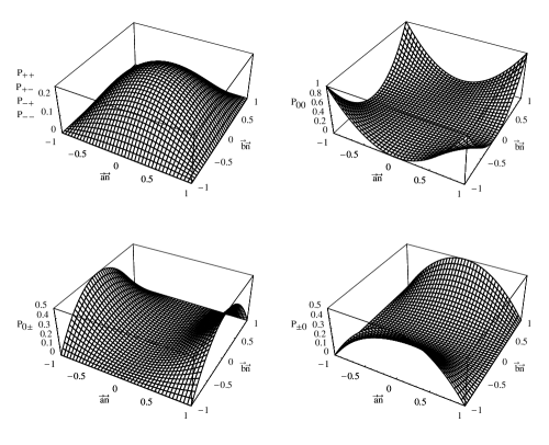
Figure 5: Dependence of probabilities (70) on $\textbf{a}\cdot\textbf{n}$ and $\textbf{b}\cdot\textbf{n}$ in the ultra-relativistic limit.

Non-relativistic limit

Now in non-relativistic limit the probabilities are

$$P_{\pm\pm} = \tfrac{1}{12}(1-(\textbf{a}\cdot\textbf{b}))^{2},$$ (72a)

$$P_{\pm\mp} = \tfrac{1}{12}(1+(\textbf{a}\cdot\textbf{b}))^{2},$$ (72b)

$$P_{0\pm}=P_{\pm 0} = \tfrac{1}{6}(1-(\textbf{a}\cdot\textbf{b})^{2}),$$ (72c)

$$P_{00} = \tfrac{1}{3}(\textbf{a}\cdot\textbf{b})^{2},$$ (72d)

and the correlation function reads

$$C_{\mathbb{ab}}=-\tfrac{2}{3}\textbf{a}\cdot\textbf{b}.$$ (73)

Let us note that in this limit probabilities and the correlation function do not depend on the momentum $\mathbb{k}$. One can also easily check that in this case they are the same as calculated in the framework of non-relativistic quantum mechanics in the singlet state

$$|\Psi\rangle=\tfrac{1}{\sqrt{3}}(|1\rangle|-1\rangle-|0\rangle|0\rangle+|-1\rangle|1\rangle),$$ (74)

where $|1\rangle$, $|0\rangle$ and $|-1\rangle$ are states with spin component along z-axis equal to $1$, $0$ and $-1$, respectively.

VII Bell-type inequalities

The spin-1 system has three degrees of freedom, which makes the full analysis of Bell inequalities much more difficult and subtle (see e.g. Chen et al. (2001a, b); Horodecki et al. (2007)). In the present paper we will show that at least for some Bell-type inequalities its violation strongly depends on the particle momenta. Moreover we discuss inequality which is satisfied for the nonrelativistic correlation function but is violated in the relativistic case.

For spin-$\tfrac{1}{2}$ particles the most commonly discussed Bell-type inequality is the Clauser-Horne-Shimony-Holt (CHSH) inequality Clauser et al. (1969):

$$|C_{\mathbb{ab}}-C_{\mathbb{ad}}|+|C_{\mathbb{cb}}+C_{\mathbb{cd}}|\leq 2$$ (75)

In (75) $C_{\mathbb{ab}}$ denotes the correlation function of spin projections on the directions a and b. One can easily check that (75) is also valid for spin-1 particles. (see e.g. Ballentine (1998)). The nonrelativistic correlation function (73) does not violate the inequality (75). Indeed, inserting (73) into (75) we get

$$|\textbf{a}\cdot\textbf{b}-\textbf{a}\cdot\textbf{d}|+|\textbf{c}\cdot\textbf{b}+\textbf{c}\cdot\textbf{d}|\leq 3.$$ (76)

The largest value of the left side of (76) is equal to $2\sqrt{2}$, therefore (76) holds in all configurations. In the relativistic framework, inserting (69) into (75) we get the following inequality:

$$\frac{1}{2+(1+2x)^{2}}\Big{\{}\Big{|}(1+2x)\big{[}(\textbf{a}\cdot\textbf{b})-(\textbf{a}\cdot\textbf{d})\big{]}\\ -2x\big{[}(\textbf{a}\cdot\textbf{n})(\textbf{b}\cdot\textbf{n})-(\textbf{a}\cdot\textbf{n})(\textbf{d}\cdot\textbf{n})\big{]}\Big{|}\\ +\Big{|}(1+2x)\big{[}(\textbf{c}\cdot\textbf{b})+(\textbf{c}\cdot\textbf{d})\big{]}\\ -2x\big{[}(\textbf{c}\cdot\textbf{n})(\textbf{b}\cdot\textbf{n})+(\textbf{c}\cdot\textbf{n})(\textbf{d}\cdot\textbf{n})\big{]}\Big{|}\Big{\}}\leq 1.$$ (77)

Our numerical simulations show that the largest value of left side of (77) is equal to 1. Therefore the CHSH inequality is not violated in the relativistic framework, either.

Therefore for spin 1 particles we have to consider other Bell-type inequalities.

According to Mermin’s paper Mermin (1980), in EPR-type experiments with a pair of spin-1 particles in the singlet state the following inequality has to be satisfied

$$C_{\mathbb{ab}}+C_{\mathbb{bc}}+C_{\mathbb{ca}}\leq 1,$$ (78)

in the theory which fulfills the assumptions of local realism. This inequality, similar to the CHSH one, is not violated in the nonrelativistic quantum mechanics. Indeed, inserting (73) into (78) we get the inequality

$$-\frac{2}{3}(\textbf{a}\cdot\textbf{b}+\textbf{b}\cdot\textbf{c}+\textbf{c}\cdot\textbf{a})\leq 1$$ (79)

which is equivalent to

$$\frac{1}{3}\big{[}3-(\textbf{a}+\textbf{b}+\textbf{c})^{2}\big{]}\leq 1.$$ (80)

The left side of (80) is largest when $\textbf{a}+\textbf{b}+\textbf{c}=\textbf{0}$. In this case (80) is of course fulfilled. Therefore nonrelativistic quantum mechanics does not violate the Bell-type inequality (78).

However, we show that the inequality (78) can be violated in the relativistic framework. Inserting (69) into inequality (78) we get

$$\frac{2}{2+(1+2x)^{2}}\Big{\{}-(1+2x)(\textbf{a}\cdot\textbf{b}+\textbf{b}\cdot\textbf{c}+\textbf{c}\cdot\textbf{a})\\ +2x\big{[}(\textbf{a}\cdot\textbf{n})(\textbf{b}\cdot\textbf{n})+(\textbf{b}\cdot\textbf{n})(\textbf{c}\cdot\textbf{n})+(\textbf{c}\cdot\textbf{n})(\textbf{a}\cdot\textbf{n})\big{]}\Big{\}}\leq 1.$$ (81)

In the configuration $\textbf{a}+\textbf{b}+\textbf{c}=\textbf{0}$, $\textbf{a}\cdot\textbf{n}=\textbf{b}\cdot\textbf{n}=\textbf{c}\cdot\textbf{n}=0$ (81) takes the form

$$\frac{3(1+2x)}{2+(1+2x)^{2}}\leq 1,$$ (82)

and one can easily check that this inequality is violated for $0<x<1/2$. (Let us note that the value $x=0$ corresponds to the nonrelativistic limit for which the inequality is not violated). The dependence of the left side of the inequality (82) is shown on the Fig. 6.

Figure 6: The plot shows dependence of the left side of the inequality (82) on $x$. The plotted function has maximum value equal to $3\sqrt{2}/4$ for $x=(\sqrt{2}-1)/2$.

In the paper Mermin (1980) another Bell-type inequality, which is violated in the nonrelativistic case, is considered. This inequality contains not only a correlation function but also the average value of the difference of spin projections measured by Alice and Bob and has the following form:

$$\sum_{\lambda,\sigma}|\lambda-\sigma|P_{\lambda\sigma}(\textbf{a},\textbf{b})\geq C_{\mathbb{ac}}+C_{\mathbb{bc}}.$$ (83)

We have calculated the probabilities $P_{\lambda\sigma}(\textbf{a},\textbf{b})$ [Eqs. (68)] therefore we can analyze the inequality (83) also in the relativistic framework. Inserting (68) and (73) into (83) we obtain the inequality

$$\frac{2}{2+(1+2x)^{2}}\Big{\{}-(1+2x)(\textbf{a}\cdot\textbf{b}+\textbf{b}\cdot\textbf{c}+\textbf{c}\cdot\textbf{a})\\ +2x\big{[}(\textbf{a}\cdot\textbf{n})(\textbf{b}\cdot\textbf{n})+(\textbf{b}\cdot\textbf{n})(\textbf{c}\cdot\textbf{n})+(\textbf{c}\cdot\textbf{n})(\textbf{a}\cdot\textbf{n})\big{]}\\ +\frac{1}{2}\big{[}(\textbf{a}\cdot\textbf{b})+2x(\textbf{a}\cdot\textbf{n})(\textbf{b}\cdot\textbf{n})\big{]}^{2}\Big{\}}\leq 1.$$ (84)

This inequality is stronger than (81). Let us analyze the inequality (84) in the configuration considered in Mermin (1980), that is let us assume that a, b, c are coplanar and $\textbf{a}\cdot\textbf{b}=\cos{(\pi-2\theta)}$, $\textbf{a}\cdot\textbf{c}=\textbf{b}\cdot\textbf{c}=\cos(\pi/2+\theta)$. Moreover let us assume that $\textbf{a}\cdot\textbf{n}=\textbf{b}\cdot\textbf{n}=\textbf{c}\cdot\textbf{n}=0$. In this configuration (84) takes the following form

$$\frac{2(1+2x)\big{[}2\sin{\theta}+\cos(2\theta)\big{]}+\cos^{2}(2\theta)}{2+(1+2x)^{2}}\leq 1.$$ (85)

We have shown the dependence of the left side of (85) on $\theta$ for two chosen vales of $x$: $x=0$ corresponding to the nonrelativistic case and $x=1/6$ on Fig. 7.

Figure 7: The plot shows dependence of the left side of the inequality (85) on $\theta$. The value $x=0$ corresponds to the nonrelativistic case The plotted function has maximum value equal to $3\sqrt{2}/4$ for $x=(\sqrt{2}-1)/2$.

We show the dependence of the left side of (85) on $x$ in Fig. (8). We have chosen $\theta=2\pi/3$ corresponding to the configuration $\textbf{a}+\textbf{b}+\textbf{c}=\textbf{0}$ considered earlier.

Figure 8: The plot shows dependence of the left side of the inequality (85) on $x$ for $\theta=2\pi/3$ corresponding to the configuration $\textbf{a}+\textbf{b}+\textbf{c}=\textbf{0}$. The plotted function has maximum value equal to $9/8$ for $x=1/6$.

Summarizing, our analysis shows that relativistic vector bosons violate Bell inequalities more than nonrelativistic spin-1 particles and that the degree of violation of the Bell inequality depends on the particle momentum.

VIII Conclusions

We have discussed joint probabilities and the correlation function of two relativistic vector bosons in the framework of quantum field theory. We have classified two-particle covariant states and defined the observables corresponding to detectors measuring the spin of the particles with momenta belonging to a given region of momentum space. Using this formalism we have explicitly calculated the correlation function and the probabilities in the scalar state. We observed strange behavior of the correlation function and the probabilities. It appears that in the CMF frame for the definite configuration of the particles momenta and directions of the spin projection measurements, the correlation function still depends on the value of the particles momenta. Recall that for two fermions the correlation function in CMF frame in the singlet state does not depend on momentum Caban and Rembieliński (2006). Furthermore, in the bosonic case for fixed spin measurement directions, the correlation function (and the probabilities) can have extrema for some finite values of the particles momenta. This affects the degree of violation of Bell-type inequalities. We have discussed the Bell-type inequality (78) which is fulfilled in the nonrelativistic limit but is violated in some finite region of the particles momenta. We have also shown that Bell-type inequality (83) which is violated for nonrelativistic spin-1 particles in the relativistic case is violated more in some finite region of the particles momenta.

Appendix A Explicit form of matrices $N^{\alpha\beta}$, $M^{\alpha\beta}$ and $T^{\alpha\beta}$

The explicit form of matrices (62) is

$$N^{\alpha\beta}(\mathbb{q},\boldsymbol{\omega})=\left(\begin{array}[]{c|c}0&\tfrac{i}{m}(\mathbb{q}\times\boldsymbol{\omega})^{\rm{T}}\\ \hline\cr-\tfrac{i}{m}(\mathbb{q}\times\boldsymbol{\omega})&-i\epsilon^{ijk}\omega^{k}+i\left[\tfrac{\mathbb{q}\otimes(\mathbb{q}\times\boldsymbol{\omega})^{\rm{T}}-(\mathbb{q}\times\boldsymbol{\omega})\otimes\mathbb{q}^{\rm{T}}}{m(m+q^{0})}\right]^{ij}\\ \end{array}\right),$$ (86a)

$$M^{\alpha\beta}(\mathbb{q},\boldsymbol{\omega})\\ =\left(\begin{array}[]{c|c}\tfrac{\mathbb{q}^{2}-(\boldsymbol{\omega}\cdot\mathbb{q})^{2}}{m^{2}}&\tfrac{\textbf{q}^{\rm{T}}}{m}\big{[}\tfrac{q^{0}}{m}-\tfrac{(\boldsymbol{\omega}\cdot\textbf{q})^{2}}{m(m+q^{0})}\big{]}-\boldsymbol{\omega}^{\rm{T}}\tfrac{\boldsymbol{\omega}\cdot\textbf{q}}{m}\\ \hline\cr\tfrac{\textbf{q}}{m}\big{[}\tfrac{q^{0}}{m}-\tfrac{(\boldsymbol{\omega}\cdot\textbf{q})^{2}}{m(m+q^{0})}\big{]}-\boldsymbol{\omega}\tfrac{\boldsymbol{\omega}\cdot\textbf{q}}{m}&{\operatorname{\openone}}-\boldsymbol{\omega}\otimes\boldsymbol{\omega}^{\rm{T}}-\tfrac{\boldsymbol{\omega}\cdot\textbf{q}}{m(m+q^{0})}\big{[}\boldsymbol{\omega}\otimes\mathbb{q}^{\rm{T}}+\mathbb{q}\otimes\boldsymbol{\omega}^{\rm{T}}\big{]}+\big{[}1-\tfrac{(\boldsymbol{\omega}\cdot\textbf{q})^{2}}{(m+q^{0})^{2}}\big{]}\tfrac{\mathbb{q}\otimes\mathbb{q}^{\rm{T}}}{m^{2}}\\ \end{array}\right),$$ (86b)

$$T^{\alpha\beta}(\mathbb{q},\boldsymbol{\omega})=\left(\begin{array}[]{c|c}\tfrac{(\boldsymbol{\omega}\cdot\textbf{q})^{2}}{m^{2}}&\tfrac{\boldsymbol{\omega}\cdot\textbf{q}}{m}\big{[}\boldsymbol{\omega}^{\rm{T}}+\tfrac{(\boldsymbol{\omega}\cdot\textbf{q})\mathbb{q}^{\rm{T}}}{m(m+q^{0})}\big{]}\\ \hline\cr\tfrac{\boldsymbol{\omega}\cdot\textbf{q}}{m}\big{[}\boldsymbol{\omega}+\tfrac{(\boldsymbol{\omega}\cdot\textbf{q})\textbf{q}}{m(m+q^{0})}\big{]}&\boldsymbol{\omega}\otimes\boldsymbol{\omega}^{\rm{T}}+\tfrac{\boldsymbol{\omega}\cdot\textbf{q}}{m(m+q^{0})}\big{[}\boldsymbol{\omega}\otimes\mathbb{q}^{\rm{T}}+\mathbb{q}\otimes\boldsymbol{\omega}^{\rm{T}}\big{]}+\tfrac{(\boldsymbol{\omega}\cdot\textbf{q})^{2}}{m^{2}(m+q^{0})^{2}}\textbf{q}\otimes\textbf{q}^{\rm{T}}\end{array}\right).$$ (86c)

References

• Nielsen and Chuang (2000) M. A. Nielsen and I. L. Chuang, Quantum Computation and Quantum Information (Cambridge University Press, Cambridge, 2000).
• Ahn et al. (2002) D. Ahn, H. J. Lee, and S. W. Hwang, Relativistic entanglement of quantum states and nonlocality of Einstein–Podolsky–Rosen(EPR) paradox, arXiv: quant-ph/0207018 (2002).
• Ahn et al. (2003a) D. Ahn, H. J. Lee, S. W. Hwang, and M. S. Kim, Is quantum entanglement invariant in special relativity?, arXiv: quant-ph/0304119 (2003a).
• Ahn et al. (2003b) D. Ahn, H. J. Lee, Y. H. Moon, and S. W. Hwang, Phys. Rev. A 67, 012103 (2003b), arXiv: quant-ph/0209164.
• Alsing and Milburn (2002) P. M. Alsing and G. J. Milburn, Quantum Information and Computation 2, 487 (2002), arXiv: quant-ph/0203051.
• Bartlett and Terno (2005) S. D. Bartlett and D. R. Terno, Phys. Rev. A 71, 012302 (2005), arXiv: quant-ph/0403014.
• Caban and Rembieliński (2003) P. Caban and J. Rembieliński, Phys. Rev. A 68, 042107 (2003), arXiv: quant-ph/0304120.
• Caban and Rembieliński (2005) P. Caban and J. Rembieliński, Phys. Rev. A 72, 012103 (2005), arXiv: quant-ph/0507056.
• Caban and Rembieliński (2006) P. Caban and J. Rembieliński, Phys. Rev. A 74, 042103 (2006), arXiv: quant-ph/0612131.
• Czachor and Wilczewski (2003) M. Czachor and M. Wilczewski, Phys. Rev. A 68, 010302(R) (2003), arXiv: quant-ph/0303077.
• Czachor (1997a) M. Czachor, Phys. Rev. A 55, 72 (1997a), arXiv: quant-ph/9609022.
• Czachor (1997b) M. Czachor, in Photonic Quantum Computing, edited by S. P. Holating and A. R. Pirich (SPIE - The International Society for Optical Engineering, Bellingham, WA, 1997b), vol. 3076 of Proceedings of SPIE, pp. 141–145, arXiv: quant-ph/0205187.
• Czachor (2005) M. Czachor, Phys. Rev. Lett. 94, 078901 (2005), arXiv: quant-ph/0312040.
• Gingrich and Adami (2002) R. M. Gingrich and C. Adami, Phys. Rev. Lett. 89, 270402 (2002), arXiv: quant-ph/0205179.
• Gingrich et al. (2003) R. M. Gingrich, A. J. Bergou, and C. Adami, Phys. Rev. A 68, 042102 (2003), arXiv: quant-ph/0302095.
• Gonera et al. (2004) C. Gonera, P. Kosiński, and P. Maślanka, Phys. Rev. A 70, 034102 (2004), arXiv: quant-ph/0310132.
• Harshman (2005) N. L. Harshman, Phys. Rev. A 71, 022312 (2005), arXiv: quant-ph/0409204.
• He et al. (2007a) S. He, S. Shao, and H. Zhang, J. Phys. A: Math. Gen. 40, F857 (2007a), arXiv: quant-ph/0701233.
• He et al. (2007b) S. He, S. Shao, and H. Zhang, Quantum Entangled Entropy: Helicity versus Spin, arXiv: quant-ph/0702028 (2007b).
• Jordan et al. (2005) T. F. Jordan, A. Shaji, and E. C. G. Sudarshan, Phys. Rev. A 73, 032104 (2006), arXiv: quant-ph/0511067.
• Jordan et al. (2006) T. F. Jordan, A. Shaji, and E. C. G. Sudarshan, Lorentz transformations that entangle spins and entangle momenta, arXiv: quant-ph/0608061 (2006).
• Kosiński and Maślanka (2003) P. Kosiński and P. Maślanka, Depurification by Lorentz boosts, arXiv: quant-ph/0310145 (2003).
• Kim and Son (2005) W. T. Kim and E. J. Son, Phys. Rev. A 71, 014102 (2005), arXiv: quant-ph/0408127.
• Li and Du (2003) H. Li and J. Du, Phys. Rev. A 68, 022108 (2003), arXiv: quant-ph/0211159.
• Li and Du (2004) H. Li and J. Du, Phys. Rev. A 70, 012111 (2004), arXiv: quant-ph/0309144.
• Lamata et al. (2006) L. Lamata, M. A. Martin-Delgado, and E. Solano, Phys. Rev. Lett. 97, 250502 (2006), arXiv: quant-ph/051208.
• Lindner et al. (2003) N. H. Lindner, A. Peres, and D. R. Terno, J. Phys. A: Math. Gen. 36, L449 (2003), arXiv: quant-ph/0304017.
• Lee and Chang-Young (2004) D. Lee and E. Chang-Young, New Journal of Physics 6, 67 (2004), arXiv: quant-ph/0308156.
• Moon et al. (2003) Y. H. Moon, D. Ahn, and S. W. Hwang, Relativistic entanglement of Bell states with general momentum, arXiv: quant-ph/0304116 (2003).
• Pachos and Solano (2003) J. Pachos and E. Solano, Quantum Information and Computation 3, 115 (2003), arXiv: quant-ph/0203065.
• Peres et al. (2002) A. Peres, P. F. Scudo, and D. R. Terno, Phys. Rev. Lett. 88, 230402 (2002), arXiv: quant-ph/0203033.
• Peres et al. (2005) A. Peres, P. F. Scudo, and D. R. Terno, Phys. Rev. Lett. 94, 078902 (2005), arXiv: quant-ph/.
• Peres and Terno (2003a) A. Peres and D. R. Terno, J. Modern Optics 50, 1165 (2003a), arXiv: quant-ph/0208128.
• Peres and Terno (2003b) A. Peres and D. R. Terno, Int. J. Quantum Information 1, 225 (2003b), arXiv: quant-ph/0301065.
• Peres and Terno (2004) A. Peres and D. R. Terno, Rev. Mod. Phys. 76, 93 (2004), arXiv: quant-ph/0212023.
• Rembieliński and Smoliński (2002) J. Rembieliński and K. A. Smoliński, Phys. Rev. A 66, 052114 (2002), arXiv: quant-ph/0204155.
• Soo and Lin (2004) C. Soo and C. C. Y. Lin, Int. J. Quantum Information 2, 183 (2004), arXiv: quant-ph/0307107.
• Terno (2003) D. R. Terno, Phys. Rev. A 67, 014102 (2003), arXiv: quant-ph/0208074.
• Terno (2005) D. R. Terno, Introduction to relativistic quantum information, arXiv: quant-ph/0508049 (2005).
• Terashima and Ueda (2003a) H. Terashima and M. Ueda, Int. J. Quantum Information 1, 93 (2003a), arXiv: quant-ph/0211177.
• Terashima and Ueda (2003b) H. Terashima and M. Ueda, Quantum Information and Computation 3, 224 (2003b), arXiv: quant-ph/0204138.
• You et al. (2004) H. You, A. M. Wang, X. Young, W. Niu, X. Ma, and F. Xu, Phys. Lett. A 333, 389 (2004), arXiv: quant-ph/0501019.
• Zbinden et al. (2001) H. Zbinden, J. Brendel, N. Gisin, and W. Tittel, Phys. Rev. A 63, 022111 (2001), arXiv: quant-ph/0007009.
• Messiah (1962) A. Messiah, Quantum mechanics (North-Holland, Amserdam, 1962).
• Bogolubov et al. (1975) N. N. Bogolubov, A. A. Logunov, and I. T. Todorov, Introduction to Axiomatic Quantum Field Theory (Benjamin, Reading, MA, 1975).
• Chen et al. (2001a) J. L. Chen, D. Kaszlikowski, L. C. Kwek, C. H. Oh, and M. Żukowski, Clauser-horne inequality for qutrits, arXiv: quant-ph/0106010 (2001a).
• Chen et al. (2001b) J. L. Chen, D. Kaszlikowski, L. C. Kwek, C. H. Oh, and M. Żukowski, Phys. Rev. A 64, 052109 (2001b).
• Horodecki et al. (2007) R. Horodecki, P. Horodecki, M. Horodecki, and K. Horodecki, Quantum entanglement, arXiv: quant-ph/0702225 (2007).
• Mermin (1980) N. D. Mermin, Phys. Rev. D 22, 356 (1980).
• Clauser et al. (1969) J. F. Clauser, M. A. Horne, A. Shimony, and R. A. Holt, Phys. Rev. Lett. 23, 880 (1969).
• Ballentine (1998) L. E. Ballentine, Quantum Mechanics (World Scientific Publishing, Singapore, 1998).