Helmet Streamers with Triple Structures:
Simulations of resistive dynamics.

Abstract

Recent observations of the solar corona with the LASCO coronagraph on board of the SOHO spacecraft have revealed the occurrence of triple helmet streamers even during solar minimum, which occasionally go unstable and give rise to large coronal mass ejections. There are also indications that the slow solar wind is either a combination of a quasi-stationary flow and a highly fluctuating component or may even be caused completely by many small eruptions or instabilities. As a first step we recently presented an analytical method to calculate simple two-dimensional stationary models of triple helmet streamer configurations. In the present contribution we use the equations of time-dependent resistive magnetohydrodynamics to investigate the stability and the dynamical behaviour of these configurations. We particularly focus on the possible differences between the dynamics of single isolated streamers and triple streamers and on the way in which magnetic reconnection initiates both small scale and large scale dynamical behaviour of the streamers. Our results indicate that small eruptions at the helmet streamer cusp may incessantly accelerate small amounts of plasma without significant changes of the equilibrium configuration and might thus contribute to the non-stationary slow solar wind. On larger time and length scales, large coronal eruptions can occur as a consequence of large scale magnetic reconnection events inside the streamer configuration. Our results also show that triple streamers are usually more stable than a single streamer.

1 Introduction

Recent observations of the corona with the LASCO coronagraph [Schwenn et al. (1997)] on board of the SOHO spacecraft showed that the corona can be highly structured even during the solar activity minimum. The observations revealed a triple structure of the streamer belt which was existent for several consecutive days. The observations further showed that these triple structures occasionally go unstable leading to a seemingly new and extraordinarily huge kind of coronal mass ejection (global CMEs). Natural questions arising from these observations are whether the helmet streamer triple structure is directly connected with or responsible for the occurrence of global CMEs and what is the physical mechanism of their formation.

The structure of helmet streamers and their stability has been studied both observationally and theoretically for a long time (e.g. pneuman:kopp71; cuperman:etal90; cuperman:etal92; koutchmy:livshits92; wang:etal93; cuperman:etal95; wu:etal95; bavassano:etal97; noci; hundhausen99). There seems to be a natural association of helmet streamers with coronal eruptions and coronal streamers are assumed to be the source region of the slow solar wind. The traditional view towards the origin of the slow solar wind is that it is a more or less stationary plasma flow on open field lines around the closed field lines of a helmet streamer. Recent observations (e.g. habbal98; noci) challenge this traditional view and indicate that the slow solar wind is non-stationary and seems to be produced and accelerated by small eruptions in the helmet streamer stalk above the cusp. This acceleration process of the slow solar wind has been compared with the rise of smoke above a burning candle (Schwenn, private communication).

Pre-SOHO observations of multiple streamer configurations during the maximum phase of solar activity and of the multiple current sheet structure of the heliospheric plasma sheet [Crooker et al. (1993), Woo et al. (1995)] have initiated several studies of the dynamics and stability of multiple current sheets with variations in only one spatial dimension [Otto and Birk (1992), Yan et al. (1994), Dahlburg and Karpen (1995), Birk et al. (1997), Wang et al. (1997)]. einaudi:etal99 have recently presented a model for the generation of the non-stationary slow solar wind based on linear and non-linear stability calculations for a single one-dimensional current sheet with field-aligned flow.

All these models do, however, in a strict sense only apply to the streamer stalk, i.e. to the open field lines of the heliospheric current sheet. Here we aim to investigate both closed and parts of the adjacent open field line regions.

Models of multiple arcade and loop structures have been investigated before by e.g. mikic:etal88, biskamp:welter89 and most recently by antiochos:etal99. Our model differs from these models basically by the possibility of having a flexible analytical initial condition for the time-dependent calculations allowing the investigation of different types of structures.

As a first step towards improving the theoretical understanding of the above mentioned phenomena in triple streamer configurations, we have calculated analytic two-dimensional static models of triple helmet streamers in a previous paper (paper1; further cited as paper I). The aim of the present paper is to undertake the next step in this investigation and to study the stability of the stationary state helmet streamer configurations calculated in paper I. We will carry this out with the help of time-dependent numerical experiments using the equations of resistive magnetohydrodynamics.

The outline of the paper is as follows. In Section 2 we discuss the basic equations and briefly describe our numerical method. Section 3 outlines our main model assumptions. In Section 4 we present the results of numerical experiments and in Section 5 we discuss our results and give an outlook on future work.

2 Basic Equations and Numerical Method

We use the equations of time-dependent resistive magnetohydrodynamics (MHD) to describe the coronal plasma. For a discussion concerning the neglect of gravity see sect. 3.1.

$$-\rho{\bf v}\cdot\nabla{\bf v}-\nabla P+{\bf j}\times{\bf B} = \rho\frac{\partial\bf v}{\partial t}$$ (1)

$$-\nabla\cdot(\rho{\bf v}) = \frac{\partial\rho}{\partial t}$$ (2)

$${\bf E}+{\bf v}\times{\bf B} = \eta{\bf j}$$ (3)

$$\nabla\cdot{\bf B} = 0$$ (4)

$${\bf j} = \frac{1}{\mu_{0}}\nabla\times{\bf B}$$ (5)

$$P = \rho RT$$ (6)

$$\frac{\partial{\bf B}}{\partial t} = -\nabla\times{\bf E}$$ (7)

$$\frac{\partial P}{\partial t}+\nabla\cdot(P{\bf v})+(\gamma-1)P\nabla\cdot{\bf v} = (\gamma-1)\eta j^{2}$$ (8)

Here, $P$ stands for the plasma pressure, $\bf B$ for the magnetic field, $\rho$ for the plasma density, $\bf v$ for the plasma velocity, $\bf E$ for the electric field, $R$ is the gas constant, $T$ the temperature, ${\bf j}$ the current density, $\eta$ the resistivity, $\gamma$ the adiabatic index and $\mu_{0}$ the vacuum permeability. We normalize the magnetic field by a typical value $B_{0}$, the plasma pressure $P$ by $B_{0}^{2}/\mu_{0}$, the mass density $\rho$ by $\rho_{0}=B_{0}^{2}/\mu_{0}\mbox{R}T$, the length $L$ by a solar radius and the current density by $B_{0}/\mu_{0}\,L$, the plasma bulk velocity by the Alfven velocity $v_{A}$, the electric field by $\frac{B_{0}^{2}}{\sqrt{\rho_{0}}}$, the time by the Alfven time and the resistivity $\eta$ by $\mu_{0}Lv_{A}$.

The time-dependent MHD equations are highly non-linear and generally are solved numerically. Our code uses an explicit finite difference scheme and is described in detail by dissjd and disslr. It has been successfully applied to several astrophysical problems (e.g. dissjd,lrtn,disslr).

One of the fundamental problems of any numerical experiment based on the non-ideal MHD equations is the strength of the resistive term. It is well-known that the level of disspation in the solar corona is very small (magnetic Reynolds number $R_{m}\simeq 10^{12}$ for Spitzer resistivity or at most a few orders magnitude lower if one allows for anomalous resistivity of some kind). This means that either the spatial resolution of the numerical code has to be large enough to resolve the small spatial length scales associated with the small disspative terms or that one has to use unrealistically large values for the dissipative coefficients. This second approach is based on the assumption that the basic dynamics of resistive processes is not changed as long as $R_{m}\gg 1$. Since the first approach cannot be carried out due to the limited capacity of modern computers, we use the second approach.

Because of the nonzero resistivity $\eta$ the MHD equations do not allow static solutions in a strict sense because of magnetic diffusion. However, it is well known that in most astrophysical plasmas the resistivity and thus the diffusive terms are very small. The diffusive time scale is in fact typically much (some orders of magnitude) larger than the dynamic time scale. As the dynamic time scale for static equilibria we take the time scale on which instabilities occur. On this time scale the magnetic diffusivity can be neglected for magnetohydrostatic equilibria in the absence of thin current sheets. If thin current sheets are present in the equilibria, magnetic diffusion on time scales short compared with typical macroscopic scales of the system might become important and lead to magnetic reconnection.

3 Model Assumptions

3.1 The initial conditions

We use the analytical stationary equilibria calculated in paper I as initial conditions for the time-dependent numerical MHD experiments. The LASCO observations (Schwenn et al., 1997) show that the streamer belt is fairly extended in azimuth. Thus we restrict our calculations to two dimensions as a first step.

As pointed out in paper I we do not include plasma flow in the stationary states of our helmet streamer configurations. The observations (e.g. habbal98) give strong evidence that a stationary slow solar wind does not exist. These observations further suggest that continuous small instabilities and eruptions lead to the formation of a non-stationary slow solar wind. It is one aim of this paper to investigate possible mechanisms which could lead to such a behaviour within the framework of our model.

We simplify the calculations by using Cartesian geometry and neglecting solar gravity. Of course, both gravity and the geometry used will have a quantitative influence on the dynamics of the system. However, the main interest of this work is to identify the possible mechanism of acceleration of the slow solar wind and the instabilities leading to coronal mass ejections in triple streamer configurations. We expect that the question whether an instability occurs or not will be dominated more by the topology of magnetic fields and less by the inclusion of gravity or by the geometry used for the calculation. The price we have to pay for making these assumptions is of course that we cannot expect a quantitative agreement of, e.g. plasma flow velocity or plasmoid velocity with the observed data. In any case the present idealized study seems necessary as a first step towards a more realistic description.

Before we investigate the resistive dynamics of helmet streamers we first have to investigate the equilibria concerning their stability within the framework of ideal MHD. Only if no significant changes of the configurations occur over many Alfvén crossing times under ideal conditions, investigations of instabilities in the framework of resistive MHD are meaningful. We investigated all configurations presented in paper I, table I and table II, numerically in the framework of ideal MHD and found that the changes in the values of kinetic energy, total energy, magnetic energy, thermal energy and total mass is less than one percent in all cases for $140$ Alfvén crossing times and thus the configurations may be regarded as ideally stable. Thus instabilities with significant plasma flow and eruptions are only to be expected if resistive effects are included. We remark that this result can be expected since the slender streamer configurations are rather close to one dimensional structures, which are known to be stable in ideal MHD Schindler et al. (1983).

3.2 Resistivity Profile

Of crucial importance for numerical experiments of resistive instabilities are the assumptions made for the dissipative terms. As we have already mentioned, the magnetic Reynolds number due to collisions in the coronal plasma is extremely large and thus the electric resistivity can usually be considered as being approximately zero. However, in localized regions with a high electric current density, plasma micro-instabilities may occur leading to an anomalous resistivity which can be several orders of magnetitude larger than the collisional resistivity. As the exact mechanisms for the generation of anomalous resistivity are still not fully known, we use ad hoc resistivity models. Fortunately, it is known from investigations of the Earth’s magnetotail Otto (1987); Otto et al. (1990) that different resistivity profiles do not influence the qualitative results significantly, while details may be different. We have investigated three different resistivity models:

1. spatially constant and time-independent resistivity,

2. spatially localized and time-independent resistivity,

3. current dependent resistivity.

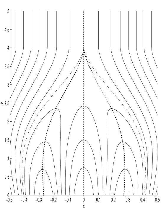
Figure 1.: Current sheets in helmet streamers. The dotted lines $\dots$ correspond to the center of each streamer and the dash-dotted lines to the separatrices between open and closed field lines. These lines are the locations where thin current sheets are likely to form.

In this paper, however, we show results mainly for the second resistivity model. The reason is that one possible mechanism to produce anomalous resistivity is the interaction of particle and waves. Candidates for such micro-instabilities are e.g. the lower hybrid drift instability and ion acoustic instability. These instabilities are well known to occur in regions with large electric current densities, e.g. thin current sheets. Figure 1 gives an overview about the location of thin current sheets within our triple helmet streamer models. Thin current sheets may form in the center of each streamer, similar to the formation of thin current sheets in the Earth’s magnetotail as investigated in e.g. wiegelmann:schindler95. Another location for thin current sheets are the separatrices between the closed field lines of helmet streamers and open field lines, because the differential rotation will cause magnetic shear on closed field lines (see paper I for details). It is thus reasonable to choose a resistivity profile which localizes the resistivity at the known locations of the strong currents. This is the case for the second and the third resistivity model. Since the difference in the results between both models turned out to be small in all cases we investigated, we decided to use the second resistivity model because it is simpler.

Therefore, in most of the results presented (except in Figure 6) we used the second resistivity model. We also performed test runs with the constant resistivity model. They gave results qualitatively similar to the other models corroborating the results of dissao and otto:etal90. Details of the resistivity models can be found in the Appendix.

4 Results of time-dependent numerical experiments

4.1 Configurations without cusp

Figure 2.: time-dependent evolution of magnetic field lines in a single streamer. The time is measured in units of the Alfvén time.

Before carrying out the numerical experiments for the triple streamer configurations, we performed a numerical experiment for a single streamer with similar parameter values. We use this experiment as a reference case. Details of the equilibrium configuration, the used grid size and the resistivity model can be found in the Appendix. Comparison of the reference case with the triple streamer cases will allow us to work out particular differences in the dynamical behaviour of the triple streamers models. Within our model, a single streamer is very similar to a model of the Earth’s magnetotail and thus our investigations of a single streamer confirm the well known results of magnetotail MHD simulations (e.g. birn80; dissao; otto:etal90). As shown in Figure 2 the configuration stretches during its evolution and after some time an X-point forms. A plasmoid appears above this X-point and is accelerated into interplanetary space. This process may be interpreted as a simple model for the development of a coronal mass ejection. In Figure 2 and in all other figures showing a time evolution the time-scale is given in units of Alfvén times $t/t_{A}$.

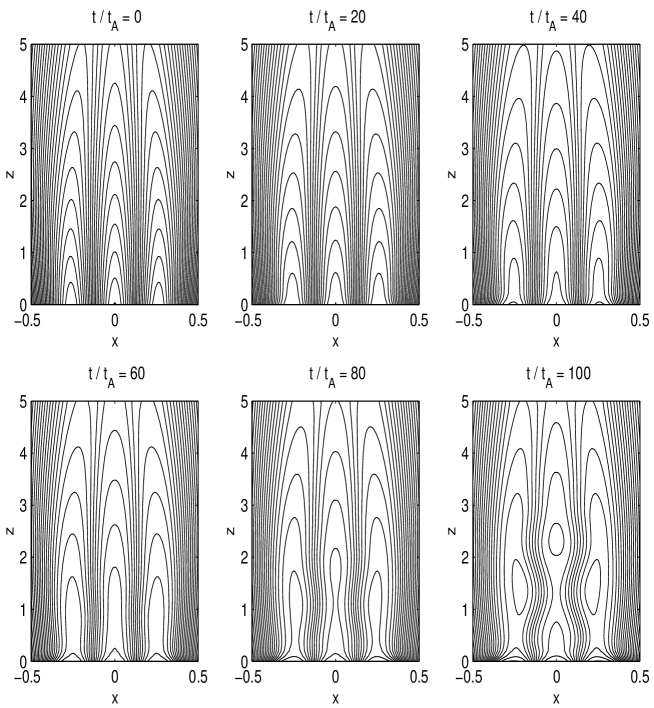
Figure 3.: Time-dependent evolution of magnetic field lines in triple streamers.

As the next example we investigate the dynamics of three parallel helmet streamers. The start configuration is given by the equilibrium with parameter set a given in Table I of paper I (see also the Appendix).

In Figure 3 we show plots of the field line evolution. As one can see in Figure 3, a plasmoid forms in all three streamers. In principle the process of plasmoid formation and acceleration in each streamer is similar to the same process in a single streamer. There are, however, some differences which we would like to point out. When we compare the triple streamer evolution with the single streamer evolution, it is conspicuous that the dynamics of the middle streamer is slower than the dynamics of the single streamer in Figure 2. Furthermore, the X-points forms somewhat higher up in the corona than in the single streamer. One also sees that the plasmoid in the middle streamer forms higher up in the corona than the plasmoids in the outer streamers. We suggest the following physical explanation for these differences between the single and triple streamer cases.

Within the process of magnetic reconnection, plasma and the frozen-in magnetic field are transported into the reconnection region. This leads to a deformation of the surrounding magnetic field outside the reconnection region as well. This deformation outside the reconnection area is not subject to changes in magnetic topology because the plasma there is frozen-in. The two outer streamers of the triple structure make this deformation of magnetic field lines much more difficult than the open field lines outside a single streamer. In our opinion, this leads to the observed slower dynamic evolution of the triple streamer configuration. This stabilizing effect of the two outer streamers towards the middle streamer is similar to the well-known boundary stabilization in other stability problems. One finds that a boundary consisting of ideally conduction walls, which are impermeable for plasma and magnetic fields, can have a stabilizing influence (for an example in the framework of solar physics see e.g. platt:neukirch94). If the separation of the boundaries parallel to the plasma sheet is small, the stabilizing effect can be so strong that no reconnection occurs. In our case the outer streamers of a triple structure are not as rigid as a conducting wall, but still much more rigid than open field lines, thus explaining the slower time evolution.

The fact that the reconnection site in the middle streamer is located higher up than in a comparable single streamer is probably again caused by the constraints imposed by the two outer streamers. The plasma flow towards the reconnection site in any of the outer streamers is only restricted on one side, while the plasma flow towards the reconnection site in the inner streamer is restricted on both sides. It is therefore no surprise that the X-points in the outer streamers form approximately at the same height as in a single streamer. This in turn leads to a deformation of the inner streamer field lines towards the outer streamers at this height. For the formation of an X-point at the same height in the middle streamer it would be necessary that the field lines deform towards the center of the middle streamer and this is just the direction opposite to their actual deformation. Thus the formation of X-points in all three streamers at the same height is impossible. As a result the formation of the X-point in the middle streamer occurs higher up in the corona than in a similar single streamer. On the other hand, the middle streamer in turn imposes geometrical restrictions on the two outer streamers. These restrictions are, however, comparatively minor and the X-points in the outer streamers form somewhat lower down than in a similar single streamer. We attribute this to the lack of symmetry within the two outer streamers.

We remark that the described effects are almost independent of the resistivity model. For the results shown in Figure 2 and 3 we used the model which localizes the resistivity in the center of the current sheet inside each streamer. Simulations with the constant resistivity model and the current dependent resistivity model lead to very similar results.

4.2 Configurations with cusp

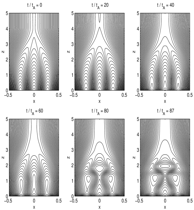
Figure 4.: Time-dependent evolution of triple streamers with cusp structure.

Pictures of helmet streamers usually show a typical cusp structure which is located at the transition from the closed field line region to the open field line region. In paper I we have calculated configurations with a cusp structure which we now use as initial conditions for our numerical experiment.

Figure 4 shows an example of the time-dependent evolution of a helmet streamer configuration with cusp structure. The initial condition is given by equilibrium a in Table II in paper I (see also Appendix). We localized the resistivity at the current sheets in the the center of each streamer and at the current sheets at the boundary between open and closed field lines (see Figure 1 for an overview about the current sheet system of triple helmet streamers).

One finds five regions within the configuration where magnetic reconnection can occur. We illustrate these processes schematically in Figure 5:

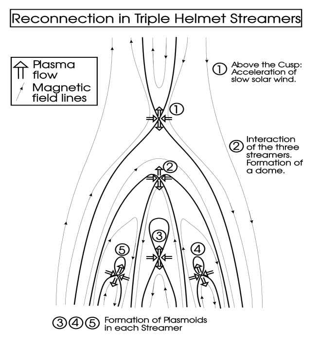
Figure 5.: Schematic illustration of processes within triple streamers with cusp.

• In the reconnection region (1) plasma and the frozen-in magnetic flux of open field lines are transported into the center and after a short time an X-point forms. At this X-point magnetic energy is transformed into kinetic energy and heat. The reconnected magnetic field above the cusp is accelerated into interplanetary space. Below the cusp a dome forms which is located above the three streamers. We suggest that reconnection processes like this one can be a significant source of plasma and magnetic flux for the wind emanating from streamer regions.

• In region (2) somewhat below the cusp we observe the following processes.

  • We find interaction between the three streamers and an X-point forms between the top parts of the two outer streamers. Above this X-point a dome forms similarly to the process (1). Below the X-point the magnetic flux of the middle streamer increases. We call this process (2a).

  • In principle this process could also happen in the opposite direction: The dome formed in region (1) is transported downward by the plasma flow. Simultaneously plasma of the middle streamer flows upward into the reconnection region around the X-point and consequently the magnetic flux of the outer streamers increases. For this process to occur it is necessary that the magnetic field configuration in the top part of the dome is flat, because for spontaneous reconnection the angle of plasma inflow has to be larger than the angle in the outflow region. We call this process (2b).

• The processes (3),(4) and (5) may occur similarly in each streamer. Plasma is transported into the center of each streamer and an X-point forms in each of these regions. A plasmoid forms inside the streamers and is accelerated. Similar to the situation of the three parallel streamers without cusp structure, the X-point in the inner streamer forms higher up in the corona than in the outer streamers.

It is useful to know which of these processes could occur simultaneously if the reconnection process was stationary. In two-dimensional configurations and for stationary magnetic reconnection it is necessary that the electric current density in the invariant direction ($j_{y}$) has the same sign in all reconnection regions (and thus in whole space). Thus stationary magnetic reconnection would be possible simultaneously for the processes (1), (2b), (4), (5) on the one hand or for the processes (2a), (3) on the other hand.

Independently of the used resistivity profile (constant, localized, current-dependent resistivity), process (1) always occurs earlier than the other processes. As the current density and thus the resistivity is assumed to be very large in the heliospheric current sheet above the cusp (see paper I for details), we also carried out numerical experiments with a localized resistivity in this area only. In that case only process (1) occurs which we tentatively identify with a possible mechanism of the acceleration of the slow solar wind in the helmet streamer stalk. The triple streamer configuration below the cusp does not change very much in this case. This corresponds to an approximately static streamer belt, from which plasma and magnetic flux are continuously expelled. Since we have not included gravitation and a possible background flow, a final assessment of the relevance of our model for the slow solar wind is not yet possible. We remark that the triple structure of the closed field line region of our streamer model does not play a major role for this process so that this process would also occur above a single streamer. The acceleration process suggested here is somewhat similar to that investigated of einaudi:etal99. The main differences are that we have not included flow in our equilibrium model, that we investigate only resistive processes and that our initial conditions are two-dimensional.

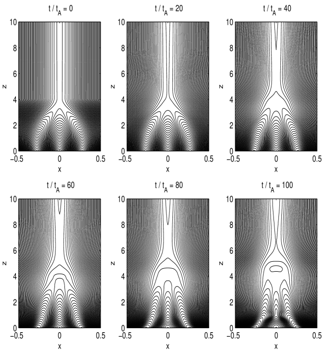
Figure 6.: Time evolution of triple helmet streamers with a different resistivity model. (note the different scales in $z$ compared with the other pictures)

For the configurations with cusp we also find that the evolution of the middle streamer is slower as compared to the evolution of a single streamer, very similar to our results for three parallel streamers without cusp. We find, however, that for the configuration with cusp the dome formed by the processes (1) and (2) has the additional effect that the plasmoid formed in the middle streamer cannot leave the configuration (and pass through the dome) without problems. The reason is that the dome has the wrong magnetic polarity to allow the plasmoid to pass by further reconnection. The plasmoid which is accelerated in process (3) is pushed against the cusp and additional reconnection processes are necessary to let it pass through the dome by processes in analogy to the process (2b). So far, however, we have not been able to find this process within our numerical experiments. One possible explanation for this is that the dome has the possibility to move outward completely without any reconnection process. The results of the numerical experiments presented in Figure 6 with a current dependent resistivity and a decreasing density profile $(\rho=p\exp(-\frac{z}{H})$ show some indications for this rise of the whole configuration including the dome. The X-point of region (1) is first located at $z=4$ and then rises to $z=7$ in the last snapshot of Figure 6. This slow rise of the dome seems to be similar to the slow coronal mass ejections observed with LASCO on SOHO Schwenn (1999); Srivastava et al. (1999) where the magnetic field lines are connected with the sun for a considerable longer time than other CME’s.

A remark is necessary concerning open and closed field lines in multiple streamer structures. In the case of parallel streamers we defined magnetic field lines as open if they cross the upper boundary. In the case of cusp solutions open field lines are outside the cusp separatrix and closed field lines inside (see paper I for details). In the case of three parallel streamers, open field lines exist between the streamers. This is not the case for for triple streamers with cusp structure. Thus configurations with cusp structure have a different magnetic topology than those without a cusp. It seems interesting to ask which of these cases is closer to reality. On the one hand, as we mentioned above, the observations often give the impression of a cusp-like structure for helmet streamers but on the other hand new observations Inhester (1998) show that within the extended streamer belt localized regions with open field lines exist. We conclude that within our two-dimensional theory we cannot model cusp-like structures and open field line regions at the same time. This shortcoming can only be overcome by a future three-dimensional model.

5 Conclusions and Outlook

In this paper we have tried to make a step towards a better theoretical understanding of the dynamics of helmet streamers with triple structure. We investigated the possible role of triple streamers for the development of coronal mass ejections and as a possible source for plasma and magnetic field for the wind emanating from streamer regions. In previous works (e.g. steinolfson94; linker94; wu:etal95; wu97 ) only single helmet streamer where modelled and these models assumed the slow solar wind as a stationary plasma flow on open field lines in the streamer region. To get a start equilibrium these authors solved the ideal time-dependent MHD equations numerically until a stationary state was reached. These works showed that helmet streamers can become unstable and produce coronal mass ejections.

The present investigations where motivated by the new observations with the LASCO coronagraph on SOHO Schwenn et al. (1997). These observations showed, that the streamer belt in the solar activity minimum typically has a triple structure. The observations also gave further strong evidence that a stationary slow solar wind may not exist but is produced by many small eruptions. Apart from these continuously occuring small eruptions, also large, however rarely occuring coronal mass ejections are generated in the triple streamer belt.

To take these observations into account in a helmet streamer model, we developed an analytical stationary model of triple helmet streamers using the ideal MHD equations in paper I. The initial states have to possess a non-vanishing free energy to allow their instability with respect to magnetic reconnection. As discussed in paper I we took into account the observation that the streamer configurations are very extended in the radial direction to simplify the calculation of the initial states. We emphasize that such radially extended configurations cannot be modeled by potential fields. In the present paper we investigated the stability of these stationary state configurations with the help numerical experiments in the framework of time-dependent resistive MHD. We used three ad hoc models for the resistivity, a constant resistivity, a resistivity localized at the thin current sheets and a current-dependent resistivity. We first investigated the ideal stability of our triple streamer configurations and found that they are stable on the time-scale of our simulations.

Next we investigated the resistive stability of a triple streamer configuration without cusp structure. We found that our triple streamer configuration is resistively unstable. Reconnection takes place and plasmoids form in each of the three closed field line regions. By comparing the time evolution of the triple streamer model with a single streamer model we found that for a triple streamer configuration without cusp structure the time-evolution is usually slower than the corresponding time evolution of a single streamer. The triple streamer evolution also shows characteristic differences in comparison with the single streamer case concerning the location of the reconnection sites. We could explain these differences by the influence the three streamers exert on each other.

For triple streamer configurations with cusp structure we found quite similar results for reconnection processes inside the closed field line regions but in addition we found that the helmet streamer stalk above the cusp is highly unstable to reconnection. This reconnection process leads to the formation of a dome above the triple structure, i.e. a region of closed field lines which encloses the triple structure completely. The resistive instability of the streamer stalk current sheet could be a possible source of plasma and magnetic field for the non-steady solar wind emanating from the streamer regions. In the present paper we have only been able to demonstrate that this mechanism works with a preexisting cusp structure. In later stages of our simulations the cusp is replaced by an X-point at which reconnection can take place. The inclusion of flow on open field lines would also allow for the possibility to generate a new cusp structure making a repetition of the process possible.

Furthermore we found interaction between the two outer streamers just below the cusp region. This interaction can also contribute to the formation of the dome. This dome makes it more difficult for plasmoids to escape and thus streamers with cusp structure within our model are less likely to eject material than the configurations without cusp.

These results are consistent with the observational finding that the triple streamer configuration is observed to be stable for several days. One may also speculate about the fact that the observations usually show three streamers which approximately have the same radial extension. A possible explanation on the basis of our model is that if one of the streamers grows and becomes much larger than the other streamers, it becomes prone to instability and a coronal mass ejection occurs similarly to the case of a single streamer. In this process the streamer looses energy, mass and magnetic flux and returns to its original state.

The numerical experiments presented here can only be considered as a very first step towards a complete model of these interesting phenomena. We already mentioned above that although the models with cusp structure seem to be matching the observed streamer structure best of all our models, it is not possible to include regions of open field lines between the streamers in our models. One way to overcome this shortcoming would be to use three-dimensional models, which is a natural next step. Other possible improvements of the present work are the inclusion of gravity and the use of spherical geometry.

It is a pleasure to thank Lutz Rastätter for supplying the numerical code used in this paper and for his help with numerical problems. We also thank Jürgen Dreher and Andreas Kopp for useful discussions of the numerical aspects of this paper and Bernd Inhester, Rainer Schwenn and Nandita Srivastava for sharing their knowledge of the LASCO observations with us. One of us (TN) is grateful to PPARC for financial support by an Advanced Fellowship.

In this section we briefly list the model parameters used for the initial streamer configurations shown in the figures and details about the grid sizes and the resistivity models.

In Figure 2 we used the model parameters $s_{1}=0.8,s_{2}=0.4,s_{3}=0.2$, $c_{1}=15$ for the initial conditions (we refer the reader to paper I, Section 3.1 for a definition of these parameters). This configuration corresponds to the middle streamer in paper I, Figures 2a and 2b. In Figure 3 we used as initial conditions the configuration a given in paper I, Table I and shown in Figure 2a of paper I. In Figure 4 we used as initial conditions the configuration a given in paper I, Table II and shown in Figure 3a of paper I.

We used a grid of $53$ points in $x$ and $z$ in Figures 2, 3, 4 and a grid of $53$ points in $x$ and $105$ points in $z$ in Figure 6. The grid is rectangular and we only calculated one half of each configuration ($x=0\dots 0.5$) and get the other half of the configurations ($x=-0.5\dots 0$) by symmetry. The coordinate $z$ runs from $0\dots 5$ in Figures 2, 3, 4 and from $0\dots 10$ in Figure 6.

In Figures 2, 3 and 4 we used a resistivity profile localized at the equilibrium current sheets shown in Figure 1. The current sheets are located in the center of each streamer and at the boundary between open and closed field lines. Thus the position of the current sheets $x_{ss}(z)$ is calculated analytically as described in paper I and the resistivity profile was chosen as $\eta=\eta_{0}\exp\left(-(x-x_{ss})^{2}/{b}\right)$ with $\eta_{0}=0.001,b=20$. In Figure 6 we used a current dependent resistivity profile in the form $\eta=\eta_{0}\exp(-a(z-z_{\mbox{cusp}}))\mbox{tanh}(|\vec{j}|)$ with $\eta_{0}=0.0005$, $a=0.1$ and $z_{\mbox{cusp}}=4$.

We mention that due to the finite grid size, there will always be small numerical fluctuations present which are superposed onto the smooth initial conditions given by the ideal equilibria. The full initial conditions are therefore given by a smooth component plus a small fluctuating part. We emphasize that we did not start the instability by adding an explicit finite amplitude perturbation to the ideal equilibria.

References

- Antiochos et al. (1999) Antiochos, S.K., DeVore, C.R. and Klimchuk, J.A.: 1999, Astrophys. J. 510, 485.
- Bavassano et al. (1997) Bavassano, B., Woo, R. and Bruno, R.: 1997 Geophys. Res. Lett. 24, 1655.
- Birk et al. (1997) Birk, G.T., Konz, C., and Otto, A.: 1997, Phys. Plasmas 4, 4173.
- Birn (1980) Birn, J.: 1980, J. Geophys. Res. 85, 1214.
- Biskamp and Welter (1989) Biskamp, D. and Welter, H.: 1989, Solar Phys. 120, 49.
- Crooker et al. (1993) Crooker, N.U., Siscoe, G.L., Shodan, S., Webb, D.F., Gosling, J.T. and Smith, E.J.: 1993, J. Geophys. Res. 98, 9371.
- Cuperman et al. (1990) Cuperman, S., Ofman, L. and Dryer, M.: 1990, Astrophys. J. 350, 846.
- Cuperman et al. (1992) Cuperman, S., Detman, T.R., Bruma, C. and Dryer, M.: 1992, Astron. Astrophys. 265, 785.
- Cuperman et al. (1995) Cuperman, S., Bruma, C., Dryer, M. and Semel, M.: 1995, Astron. Astrophys. 299, 389.
- Dahlburg and Karpen (1995) Dahlburg, R.B. and Karpen, J.T.: 1995, J. Geophys. Res. 100, 23489.
- Dreher (1997) Dreher, J.: 1997, PhD Thesis, Ruhr-Universität Bochum.
- Einaudi et al. (1999) Einaudi, G., Boncinelli, P., Dahlburg, R.B. and Karpen, J.T.: 1999, J. Geophys. Res. 104, 521.
- Habbal et al. (1997) Habbal, S.R., Woo, R., Fineschi, S., Neal, R.O., Kohl, J., Noci, G. and Korendyke, C.: 1997, Astrophys. J. Lett. 489, L103.
- Hundhausen (1999) Hundhausen, A.J.: 1999, in K. Strong, J. Saba, B. Haisch and J. Schmelz (eds.), The Many Faces of the Sun, Springer, 143.
- Inhester (1998) Inhester, B.: 1998, personal communication.
- Koutchmy and Livshits (1992) Koutchmy, S. and Livshits, M.: 1992, Space Sci. Rev. 61, 393.
- Linker and Mikic. (1995) Linker, J.A. und Mikic, Z.: 1995, ApJ438, L45-L48
- Mikic et al. (1988) Mikic, Z., Barnes, D.C. and Schnack, D.D.: 1988, Astrophys. J. 328, 830.
- Noci et al. (1997) Noci, G., Kohl, J.L., Antonucci, E. Tondello, G., Huber, M.C.E. et al.: 1997 Proceedings of Fifth SOHO Workshop ESA SP-404, 75.
- Otto (1987) Otto, A.: 1987, PhD Thesis, Ruhr-Universität Bochum.
- Otto and Birk (1992) Otto, A. and Birk, G.T.: 1992, Phys. Fluids B 4, 3811.
- Otto et al. (1990) Otto, A., Schindler, K. and Birn, J.: 1990, J. Geophys. Res. 95, 15023.
- Platt and Neukirch (1994) Platt, U. and Neukirch, T.: 1994, Solar Phys. 153, 287.
- Pneuman and Kopp (1971) Pneuman, G.W. and Kopp, R.A.: 1971, Solar Phys. 18, 258.
- Rastätter (1997) Rastätter, L.: 1997, PhD Thesis, Ruhr-Universität Bochum.
- Rastätter and Neukirch (1997) Rastätter, L. and Neukirch, T.: 1997, Astronomy and Astrophysics 323, 923.
- Schindler et al. (1983) Schindler, K., Birn, J. and Janicke, L.: 1983, Solar Phys. 87, 103.
- Schwenn et al. (1997) Schwenn, R., Inhester, B., Plunkett, S.P., Epple, A., Podlipnik, B., et al.: 1997, Solar Phys., 175, 667.
- Schwenn (1999) Schwenn, R.: 1999, Proceedings Plastro 98, in press.
- Srivastava et al. (1999) Srivastava, N., Schwenn, R., Inhester, B., Stenborg G., and Podlipnik, B., Solar Wind Nine, AIP CP 471 edited by S. R. Habbal, R. Esser, J. V. Hollweg and P. A. Isenberg, pp. 115-118, New York, 1999
- Steinolfson (1994) Steinolfson, R.S.: 1994, Space Sci. Rev. 70, 289.
- Wang et al. (1993) Wang, A.-H., Wu, S.T., Suess, S.T. and Poletto, G.: 1993, Solar Phys. 147, 55.
- Wang et al. (1997) Wang, S., Liu, Y.F. and Zheng, H.N.: 1997, Solar Phys. 173, 409.
- Wiegelmann and Schindler (1995) Wiegelmann, T. and Schindler, K.: 1995, Geophys. Res. Lett. 22, 2057.
- Wiegelmann et al. (1998) Wiegelmann, T., Schindler, K. and Neukirch, T.: 1998, Solar Phys.180, 439.
- Woo et al. (1995) Woo, R., Armstrong, J.W., Bird, M.K. and Pätzold, M.: 1995, Astrophys. J. 449, L91.
- Wu et al. (1995) Wu, S.T., Guo, W.P. and Wang, J.F.: 1995, Solar Phys. 157, 325.
- Wu and Guo (1997) Wu, S.T., Guo, W.P.: 1997, in Coronal Mass Ejections: Causes and Consequences (N. Crooker, J. Joselyn and J. Feynman eds.) AGU Geophysical Monograph Series, American Geophysical Union, Washington, DC, 1997
- Yan et al. (1994) Yan, M., Otto, A., Muzzell, D. and Lee, L.C.: 1994, J. Geophys. Res. 97, 16789.