Towards optimal DRP scheme for linear advection

Abstract

Finite difference schemes are here solved by means of a linear matrix equation. The theoretical study of the related algebraic system is exposed, and enables us to minimize the error due to a finite difference approximation, while building a new DRP scheme in the same time.

keywords
DRP schemes, Sylvester equation

1 Introduction: Scheme classes

We hereafter propose a method that enables us to build a DRP scheme while minimizing the error due to the finite difference approximation, by means of an equivalent matrix equation.

Consider the transport equation:

$$\frac{\partial u}{\partial t}+c\,\frac{\partial u}{\partial x}=0\,\,\,,\,\,\,x\,\in\,[0,L],\,\,\,t\,\in\,[0,T]$$ (1)

with the initial condition $u(x,t=0)=u_{0}(x)$.

Proposition 1.1

A finite difference scheme for this equation can be written under the form:

$${{{{{\alpha\,u}}_{i}}}^{n+1}}+{{{{{\beta\,u}}_{i}}}^{n}}+{{{{{\gamma\,u}}_{i}}}^{n-1}}+\delta\,{{{u_{i+1}}}^{n}}+{{{{{\varepsilon\,u}}_{i-1}}}^{n}}+{{{{{\zeta\,u}}_{i+1}}}^{n+1}}+{{{{{\eta\,u}}_{i-1}}}^{n-1}}+{{{{{\theta\,u}}_{i-1}}}^{n+1}}+\vartheta\,{{u}_{i+1}}^{n-1}=0$$ (2)

where:

$${u_{l}}^{m}=u\,(l\,h,m\,\tau)$$ (3)

$l\,\in\,\{i-1,\,i,\,i+1\}$, $m\,\in\,\{n-1,\,n,\,n+1\}$, $j=0,\,...,\,n_{x}$, $n=0,\,...,\,n_{t}$, $h$, $\tau$ denoting respectively the mesh size and time step ($L=n_{x}\,h$, $T=n_{t}\,\tau$).
The Courant-Friedrichs-Lewy number ($cfl$) is defined as $\sigma=c\,\tau/h$ .

A numerical scheme is specified by selecting appropriate values of the coefficients $\alpha$, $\beta$, $\gamma$, $\delta$, $\varepsilon$, $\zeta$, $\eta$, $\theta$ and $\vartheta$ in equation (2), which, for sake of usefulness, will be written as:

$$\alpha=\alpha_{x}+\alpha_{t}\,\,\,,\,\,\,\beta=\beta_{x}+\beta_{t}\,\,\,,\,\,\,\gamma=\gamma_{x}+\gamma_{t}\,\,\,,\,\,\,\delta=\delta_{x}+\delta_{t}\,\,\,,\,\,\,\varepsilon=\varepsilon_{x}+\varepsilon_{t}\,\,\,,\,\,\,$$ (4)

where the ”_x” denotes a dependance upon the mesh size $h$, while the ”_t” denotes a dependance upon the time step $\tau$.

The number of time steps will be denoted $n_{t}$, the number of space steps, $n_{x}$. In general, $n_{x}\gg n_{t}$.

In the following: the only dependance of the coefficients upon the time step $\tau$ existing only in the Crank-Nicolson scheme, we will restrain our study to the specific case:

$$\alpha_{t}=\gamma_{t}=\zeta=\eta=\theta=\vartheta=0$$ (5)

The paper is organized as follows. The building of the DRP scheme is exposed in section 2. The equivalent matrix equation, which enables us to minimize the error due to the finite difference approximation, is presented in section 3. A numerical example is given in section LABEL:Ex.

2 The DRP scheme

The first derivative $\frac{\partial u}{\partial x}$ is approximated at the $l^{th}$ node of the spatial mesh by:

$$(\,\frac{\partial u}{\partial x}\,)_{l}\simeq{{{{{\beta_{x}\,u}}_{l+i}}}^{n}}+\delta_{x}\,{{{u_{l+i+1}}}^{n}}+{{{{{\varepsilon_{x}\,u}}_{l+i-1}}}^{n}}$$ (6)

Following the method exposed by C. Tam and J. Webb in [1], the coefficients $\beta_{x}$, $\delta_{x}$, and $\varepsilon_{x}$ are determined requiring the Fourier Transform of the finite difference scheme (6) to be a close approximation of the partial derivative $(\,\frac{\partial u}{\partial x}\,)_{l}$.
(6) is a special case of:

$$(\,\frac{\partial u}{\partial x}\,)_{l}\simeq\beta_{x}\,u(x+i\,h)+\delta_{x}\,u(x+(i+1)\,h)+\varepsilon_{x}\,u(x+(i-1)\,h)$$ (7)

where $x$ is a continuous variable, and can be recovered setting $x=l\,h$.
Denote by $\omega$ the phase. Applying the Fourier transform, referred to by $\,\widehat{\,}$ , to both sides of (7), yields:

$$j\,\omega\,\widehat{u}\simeq\left\{\beta_{x}\,e^{\,0}+\delta_{x}\,e^{\,j\,\omega\,h}+\varepsilon_{x}\,e^{\,-\,j\,\omega\,h}\right\}\,\widehat{u}$$ (8)

$j$ denoting the complex square root of $-1$.

Comparing the two sides of (8) enables us to identify the wavenumber $\overline{\lambda}$ of the finite difference scheme (6) and the quantity $\frac{1}{j}\,\left\{\beta_{x}\,e^{\,0}+\delta_{x}\,e^{\,j\,\omega\,h}+\varepsilon_{x}\,e^{\,-\,j\,\omega\,h}\,\right\}$, i. e.: The wavenumber of the finite difference scheme (6) is thus:

$$\overline{\lambda}=-\,j\,\left\{\beta_{x}\,e^{\,0}+\delta_{x}\,e^{\,j\,\omega\,h}+\varepsilon_{x}\,e^{\,-\,j\,\omega\,h}\,\right\}$$ (9)

To ensure that the Fourier transform of the finite difference scheme is a good approximation of the partial derivative $(\,\frac{\partial u}{\partial x}\,)_{l}$ over the range of waves with wavelength longer than $4\,h$, the a priori unknowns coefficients $\beta_{x}$, $\delta_{x}$, and $\varepsilon_{x}$ must be choosen so as to minimize the integrated error:

$$\begin{array}[]{rcl}{\mathcal{E}}&=&\int_{-\frac{\pi}{2}}^{\frac{\pi}{2}}|\lambda\,h-\overline{\lambda}\,h|^{2}\,d(\lambda\,h)\\ &=&\int_{-\frac{\pi}{2}}^{\frac{\pi}{2}}|\kappa+j\,h\,\left\{\beta_{x}\,e^{\,0}+\delta_{x}\,e^{\,j\,\kappa}+\varepsilon_{x}\,e^{\,-\,j\,\kappa}\,\right\}\,|^{2}\,d(\kappa)\end{array}$$ (10)

The conditions that ${\mathcal{E}}$ is a minimum are:

$$\frac{\partial{\mathcal{E}}}{\partial\beta_{x}}=\frac{\partial{\mathcal{E}}}{\partial\delta_{x}}=\frac{\partial{\mathcal{E}}}{\partial\varepsilon_{x}}=0$$ (11)

and provide the following system of linear algebraic equations:

$$\left\{\begin{array}[]{rcl}2\,\pi\,h\,\beta_{x}+4\,(h\,\delta_{x}+h\,\varepsilon_{x}-1)&=&0\\ 4\,h\,\beta_{x}+\pi\,(2\,\delta_{x}-1)&=&0\\ 4\,h\,\beta_{x}+2\,\pi\,h\,\varepsilon_{x}&=&0\end{array}\right.$$ (12)

which enables us to determine the required values of $\beta_{x}$, $\delta_{x}$, and $\varepsilon_{x}$:

$$\left\{\begin{array}[]{rcl}\beta_{x}&=&\beta_{x}^{opt}\,=\,\frac{\pi}{h\,(\pi^{2}-8)}\\ \delta_{x}&=&\delta_{x}^{opt}\,=\,\frac{1}{2}-\frac{2}{h\,(\pi^{2}-8)}\\ \varepsilon_{x}&=&\varepsilon_{x}^{opt}\,=\,-\frac{2}{h\,(\pi^{2}-8)}\\ \end{array}\right.$$ (13)

3 The Sylvester equation

3.1 Matricial form of the finite differences problem

Theorem 3.1

The problem (2) can be written under the following matricial form:

$${M_{1}}\,U+U\,M_{2}+{\cal{L}}(U)=M_{0}$$ (14)

where $M_{1}$ and $M_{2}$ are square matrices respectively $n_{x}-1$ by $n_{x}-1$, $n_{t}$ by $n_{t}$, given by:

$$\begin{array}[]{ccc}{M_{1}}=\left(\begin{array}[]{ccccc}\beta&\delta&0&\ldots&0\\ \varepsilon&\beta&\ddots&\ddots&\vdots\\ 0&\ddots&\ddots&\ddots&0\\ \vdots&\ddots&\ddots&\beta&\delta\\ 0&\ldots&0&\varepsilon&\beta\\ \end{array}\right)&&{M_{2}}=\left(\begin{array}[]{ccccc}0&\gamma&0&\ldots&0\\ \alpha&0&\ddots&\ddots&\vdots\\ 0&\ddots&\ddots&\ddots&0\\ \vdots&\ddots&\ddots&\ddots&\gamma\\ 0&\ldots&0&\alpha&0\\ \end{array}\right)\end{array}$$ (15)

the matrix $M_{0}$ being given by:

$$\scriptsize{{M_{0}}=\left(\begin{array}[]{ccccc}-\gamma\,u_{1}^{0}-\varepsilon\,u_{0}^{1}-\eta\,u_{0}^{0}-\theta\,u_{0}^{2}-\vartheta\,u_{2}^{0}&-\varepsilon\,u_{0}^{2}-\eta\,u_{0}^{1}-\theta\,u_{0}^{3}&\ldots&\ldots&-\varepsilon\,u_{0}^{n_{t}}-\eta\,u_{0}^{n_{t}-1}\\ -\gamma\,u_{2}^{0}-\eta\,u_{1}^{0}-\vartheta\,u_{3}^{0}&0&\ldots&\ldots&0\\ \vdots&\vdots&\vdots&\vdots&\vdots\\ -\gamma\,u_{n_{x}-2}^{0}-\eta\,u_{n_{x}-2}^{0}-\vartheta\,u_{n_{x}-1}^{0}&0&\ldots&\ldots&0\\ -\gamma\,u_{n_{x}-1}^{0}-\delta\,u_{n_{x}}^{1}-\eta\,u_{n_{x}-2}^{0}-\zeta\,u_{n_{x}}^{2}-\vartheta\,u_{n_{x}}^{0}&-\delta\,u_{n_{x}}^{2}-\zeta\,u_{n_{x}}^{3}-\vartheta\,u_{n_{x}}^{1}&\ldots&\ldots&-\delta\,u_{n_{x}}^{n_{t}}-\vartheta\,u_{n_{x}}^{n_{t}-1}\\ \end{array}\right)}$$ (16)

and where ${\cal{L}}$ is a linear matricial operator which can be written as:

$${\cal{L}}={\cal{L}}_{1}+{\cal{L}}_{2}+{\cal{L}}_{3}+{\cal{L}}_{4}$$ (17)

where ${\cal{L}}_{1}$, ${\cal{L}}_{2}$, ${\cal{L}}_{3}$ and ${\cal{L}}_{4}$ are given by:

$$\begin{array}[]{ccc}{\cal{L}}_{1}(U)=\zeta\left(\begin{array}[]{ccccc}u_{2}^{2}&u_{2}^{3}&\ldots&u_{2}^{n_{t}}&0\\ u_{3}^{2}&u_{3}^{3}&\ldots&\vdots&\vdots\\ \vdots&\vdots&\ddots&\vdots&\vdots\\ u_{n_{x}-1}^{2}&u_{n_{x}-1}^{3}&\ldots&u_{n_{x}-1}^{n_{t}}&0\\ 0&0&\ldots&0&0\\ \end{array}\right)&&{\cal{L}}_{2}(U)=\eta\left(\begin{array}[]{ccccc}0&0&\ldots&0&0\\ 0&u_{1}^{1}&u_{1}^{2}&\ldots&u_{1}^{n_{t}-1}\\ 0&u_{1}^{0}&u_{1}^{1}&\ldots&u_{2}^{n_{t}-1}\\ \vdots&\vdots&\vdots&\ddots&\vdots\\ 0&u_{n_{x}-2}^{1}&u_{n_{x}-2}^{2}&\ldots&u_{n_{x}-2}^{n_{t}-1}\\ \end{array}\right)\end{array}$$ (18)

$$\begin{array}[]{ccc}{\cal{L}}_{3}(U)=\theta\left(\begin{array}[]{ccccc}0&\ldots&\ldots&\ldots&0\\ u_{1}^{2}&u_{1}^{3}&\ldots&u_{1}^{n_{t}}&0\\ u_{2}^{2}&u_{2}^{3}&\ldots&u_{2}^{n_{t}}&0\\ \vdots&\vdots&\vdots&\vdots&\vdots\\ u_{n_{x}-2}^{2}&u_{n_{x}-2}^{3}&\ldots&u_{n_{x}-2}^{n_{t}}&0\\ \end{array}\right)&&{\cal{L}}_{4}(U)=\vartheta\left(\begin{array}[]{ccccc}0&u_{2}^{1}&u_{2}^{2}&\ldots&u_{2}^{n_{t}-1}\\ 0&u_{3}^{1}&u_{3}^{2}&\ldots&u_{3}^{n_{t}-1}\\ \vdots&\vdots&\ddots&\ddots&\vdots\\ 0&u_{n_{x}-1}^{1}&\ldots&\ldots&u_{n_{x}-1}^{n_{t}-1}\\ 0&0&\ldots&\ldots&0\\ \end{array}\right)\end{array}$$ (19)

Proposition 3.2

The second member matrix $M_{0}$ bears the initial conditions, given for the specific value $n=0$, which correspond to the initialization process when computing loops, and the boundary conditions, given for the specific values $i=0$, $i=n_{x}$.

Denote by $u_{exact}$ the exact solution of (1).
The corresponding matrix $U_{exact}$ will be:

$$U_{exact}=[{{{U_{{exact}_{i}}}}^{n}}{]_{\,1\leq i\leq{n_{x}-1},\,1\leq n\leq{n_{t}}\,}}$$ (20)

where:

$${U_{exact}}_{i}^{n}=U_{exact}(x_{i},t_{n})$$ (21)

with $x_{i}=i\;h$, $t_{n}=n\;\tau$.

Definition 3.3

We will call error matrix the matrix defined by:

$$E=U-U_{exact}$$ (22)

Consider the matrix $F$ defined by:

$$F={M_{1}}\,U_{exact}+U_{exact}\,M_{2}+{\cal{L}}(U_{exact})-M_{0}$$ (23)

Proposition 3.4

The error matrix $E$ satisfies:

$${M_{1}}\,E+E\,M_{2}+{\cal{L}}(E)=F$$ (24)

3.2 The matrix equation

Theorem 3.5

Minimizing the error due to the approximation induced by the numerical scheme is equivalent to minimizing the norm of the matrices $E$ satisfying (24).

Note: Since the linear matricial operator ${\cal{L}}$ appears only in the Crank-Nicolson scheme, we will restrain our study to the case ${\cal{L}}=0$. The generalization to the case ${\cal{L}}\neq 0$ can be easily deduced.

Proposition 3.6

The problem is then the determination of the minimum norm solution of:

$${M_{1}}\,E+E\,M_{2}=F$$ (25)

which is a specific form of the Sylvester equation:

$$AX+XB=C$$ (26)

where $A$ and $B$ are respectively $m$ by $m$ and $n$ by $n$ matrices, $C$ and $X$, $m$ by $n$ matrices.

3.3 Minimization of the error

Calculation yields:

$$\left\{\begin{array}[]{ccc}{M_{1}}\,^{T}M_{1}&=&diag\big{(}\left(\begin{array}[]{cc}\beta^{2}+\delta^{2}&\beta\,(\delta+\varepsilon)\\ \beta\,(\delta+\varepsilon)&\varepsilon^{2}+\beta^{2}\\ \end{array}\right),\ldots,\left(\begin{array}[]{cc}\beta^{2}+\delta^{2}&\beta\,(\delta+\varepsilon)\\ \beta\,(\delta+\varepsilon)&\varepsilon^{2}+\beta^{2}\\ \end{array}\right)\big{)}\\ {M_{2}}\,^{T}M_{2}&=&diag\big{(}\left(\begin{array}[]{cc}\gamma^{2}&0\\ 0&\alpha^{2}\\ \end{array}\right),\ldots,\left(\begin{array}[]{cc}\gamma^{2}&0\\ 0&\alpha^{2}\\ \end{array}\right)\end{array}\right.$$ (27)

The singular values of $M_{1}$ are the singular values of the block matrix $\big{(}\left(\begin{array}[]{cc}\beta^{2}+\delta^{2}&\beta\,(\delta+\varepsilon)\\ \beta\,(\delta+\varepsilon)&\varepsilon^{2}+\beta^{2}\\ \end{array}\right)$, i. e.

$$\frac{1}{2}\,(2\beta^{2}+\delta^{2}+\varepsilon^{2}-(\delta+\varepsilon)\,\sqrt{4\beta^{2}+\delta^{2}+\varepsilon^{2}-2\delta\,\varepsilon})$$ (28)

of order $\frac{n_{x}-1}{2}$, and

$$\frac{1}{2}\,(2\beta^{2}+\delta^{2}+\varepsilon^{2}+(\delta+\varepsilon)\,\sqrt{4\beta^{2}+\delta^{2}+\varepsilon^{2}-2\delta\,\varepsilon})$$ (29)

of order $\frac{n_{x}-1}{2}$.

The singular values of $M_{2}$ are $\alpha^{2}$, of order $\frac{n_{t}}{2}$, and $\gamma^{2}$, of order $\frac{n_{t}}{2}$.

Consider the singular value decomposition of the matrices $M_{1}$ and $M_{2}$:

$$U_{1}^{T}\,M_{1}\,V_{1}=\left(\begin{array}[]{cc}\widetilde{M_{1}}&0\\ 0&0\\ \end{array}\right)\,\,\,,\,\,\,U_{2}^{T}\,M_{1}\,V_{2}=\left(\begin{array}[]{cc}\widetilde{M_{2}}&0\\ 0&0\\ \end{array}\right)$$ (30)

where $U_{1}$, $V_{1}$, $U_{2}$, $V_{2}$, are orthogonal matrices. $\widetilde{M_{1}}$, $\widetilde{M_{2}}$ are diagonal matrices, the diagonal terms of which are respectively the nonzero eigenvalues of the symmetric matrices $M_{1}\,^{T}M_{1}$, $M_{2}\,^{T}M_{2}$.

Multiplying respectively 25 on the left side by ${}^{T}U_{1}$, on the right side by $V_{2}$, yields:

$$U_{1}^{T}\,M_{1}\,E\,V_{2}+U_{1}^{T}\,E\,M_{2}\,V_{2}=U_{1}^{T}\,F\,V_{2}$$ (31)

which can also be taken as:

$${}^{T}U_{1}\,M_{1}\,V_{1}\,^{T}V_{1}\,E\,V_{2}+^{T}U_{1}\,E\,^{T}U_{2}\,^{T}U_{2}\,M_{2}\,V_{2}=U_{1}^{T}\,F\,V_{2}$$ (32)

Set:

$${}^{T}V_{1}\,E\,V_{2}=\left(\begin{array}[]{cc}\widetilde{E_{11}}&\widetilde{E_{12}}\\ \widetilde{E_{21}}&\widetilde{E_{22}}\\ \end{array}\right)\,,\,^{T}U_{1}\,E\,^{T}U_{2}=\left(\begin{array}[]{cc}\widetilde{\widetilde{E_{11}}}&\widetilde{\widetilde{E_{12}}}\\ \widetilde{\widetilde{E_{21}}}&\widetilde{\widetilde{E_{22}}}\\ \end{array}\right)$$ (33)

$$^{T}U_{1}\,F\,V_{2}=\left(\begin{array}[]{cc}\widetilde{F_{11}}&\widetilde{F_{12}}\\ \widetilde{F_{21}}&\widetilde{F_{22}}\\ \end{array}\right)$$ (34)

We have thus:

$$\left(\begin{array}[]{cc}\widetilde{M_{1}}\,\widetilde{E_{11}}&\widetilde{M_{1}}\,\widetilde{E_{12}}\\ 0&0\\ \end{array}\right)+\left(\begin{array}[]{cc}\widetilde{\widetilde{E_{11}}}\,\widetilde{M_{2}}&0\\ \widetilde{\widetilde{E_{21}}}\,\widetilde{M_{2}}&0\\ \end{array}\right)=\left(\begin{array}[]{cc}\widetilde{F_{11}}&\widetilde{F_{12}}\\ \widetilde{F_{21}}&\widetilde{F_{22}}\\ \end{array}\right)$$ (35)

It yields:

$$\left\{\begin{array}[]{ccc}\widetilde{M_{1}}\,\widetilde{E_{11}}+\widetilde{\widetilde{E_{11}}}\,\widetilde{M_{2}}&=&\widetilde{F_{11}}\\ \widetilde{M_{1}}\,\widetilde{E_{12}}&=&\widetilde{F_{12}}\\ \widetilde{\widetilde{E_{21}}}\,\widetilde{M_{2}}&=&\widetilde{F_{21}}\\ \end{array}\right.$$ (36)

One easily deduces:

$$\left\{\begin{array}[]{ccc}\widetilde{E_{12}}&=&{\widetilde{M}_{1}}^{-1}\,\widetilde{F_{12}}\\ {\widetilde{\widetilde{E}_{21}}}&=&\widetilde{F_{21}}\,{\widetilde{M_{2}}}^{-1}\\ \end{array}\right.$$ (37)

The problem is then the determination of the $\widetilde{E_{11}}$ and $\widetilde{\widetilde{E_{11}}}$ satisfying:

$$\widetilde{M_{1}}\,\widetilde{E_{11}}+\widetilde{\widetilde{E_{11}}}\,\widetilde{M_{2}}=\widetilde{F_{11}}$$ (38)

Denote respectively by $\widetilde{e_{ij}}$, $\widetilde{\widetilde{e_{ij}}}$ the components of the matrices $\widetilde{E}$, $\widetilde{\widetilde{E}}$.
The problem 38 uncouples into the independent problems:
minimize

$$\sum_{i,j}{\widetilde{e_{ij}}}^{2}+{\widetilde{\widetilde{e_{ij}}}}^{2}$$ (39)

under the constraint

$$\widetilde{M_{1}}_{ii}\,{\widetilde{e_{ij}}}+\widetilde{M_{2_{ii}}}\,{\widetilde{\widetilde{e_{ij}}}}=\widetilde{F_{11}}_{ij}$$ (40)

This latter problem has the solution:

$$\left\{\begin{array}[]{ccc}\widetilde{e_{ij}}&=&\frac{\widetilde{{M_{1}}_{ii}}\,\widetilde{{F_{11}}_{ij}}}{{\widetilde{{M_{1}}_{ii}}}^{2}+{\widetilde{{M_{2}}_{jj}}^{2}}}\\ \widetilde{\widetilde{e_{ij}}}&=&\frac{\widetilde{{M_{2}}_{jj}}\,\widetilde{{F_{11}}_{ij}}}{{\widetilde{{M_{1}}_{ii}}}^{2}+{\widetilde{{M_{2}}_{jj}}^{2}}}\\ \end{array}\right.$$ (41)

The minimum norm solution of 25 will then be obtained when the norm of the matrix $\widetilde{{F_{11}}}$ is minimum.
In the following, the euclidean norm will be considered.

Due to (34):

$$\|\widetilde{{F_{11}}}\|\leq\|\widetilde{{F}}\|\leq\|U_{1}\|\,\|F\|\,\|V_{2}\|\leq\|U_{1}\|\,\|V_{2}\|\,\|M_{1}\,U_{exact}+U_{exact}\,M_{2}-M_{0}\|$$ (42)

$U_{1}$ and $V_{2}$ being orthogonal matrices, respectively $n_{x}-1$ by $n_{x}-1$, $n_{t}$ by $n_{t}$, we have:

$$\|U_{1}\|^{2}=n_{x}-1\,\,\,,\,\,\,\|V_{2}\|^{2}=n_{t}$$ (43)

Also:

$$\|M_{1}\|^{2}=\frac{n_{x}-1}{2}\,\big{(}2\,\beta^{2}+\delta^{2}+\varepsilon^{2}\big{)}\,\,\,,\,\,\,\|M_{2}\|^{2}=\frac{n_{t}}{2}\,\big{(}\alpha^{2}+\gamma^{2}\big{)}$$ (44)

The norm of $M_{0}$ is obtained thanks to relation (16).

This results in:

$$\|\widetilde{{F_{11}}}\|\leq\sqrt{n_{t}\,(n_{x}-1)}\,\left\{\|U_{exact}\|\,\big{(}\sqrt{\frac{n_{x}-1}{2}}\,\sqrt{2\,\beta^{2}+\delta^{2}+\varepsilon^{2}}+\sqrt{\frac{n_{t}}{2}}\,\sqrt{\alpha^{2}+\gamma^{2}}\,\big{)}+\|M_{0}\|\right\}$$ (45)

$\|\widetilde{{F_{11}}}\|$ can be minimized through the minimization of the second factor of the right-side member of (45), which is function of the scheme parameters.

$\|U_{exact}\|$ is a constant. The quantities $\sqrt{\frac{n_{x}-1}{2}}\,\sqrt{2\,\beta^{2}+\delta^{2}+\varepsilon^{2}}$, $\sqrt{\alpha^{2}+\gamma^{2}}$ and $\|M_{0}\|$ being strictly positive, minimizing the second factor of the right-side member of (45) can be obtained through the minimization of the following functions:

$$\left\{\begin{array}[]{rcl}f_{1}(\beta,\delta,\varepsilon)&=&\sqrt{2\,\beta^{2}+\delta^{2}+\varepsilon^{2}}\\ f_{2}(\alpha,\gamma)&=&\sqrt{\alpha^{2}+\gamma^{2}}\\ f_{3}(\alpha,\beta,\gamma,\delta,\varepsilon)&=&\|M_{0}\|\\ \end{array}\right.$$ (46)

i.e.:

$$\left\{\begin{array}[]{rcl}f_{1}(\beta,\delta,\varepsilon)&=&\sqrt{2\,(\beta_{x}+\beta_{t})^{2}+(\delta_{x}+\delta_{t})^{2}+(\varepsilon_{x}+\varepsilon_{t})^{2}}\\ f_{2}(\alpha,\gamma)&=&\sqrt{\alpha_{x}^{2}+\gamma_{x}^{2}}\\ f_{3}(\alpha,\beta,\gamma,\delta,\varepsilon)&=&\|M_{0}\|\\ \end{array}\right.$$ (47)

Setting:

$$\left\{\begin{array}[]{rcl}\beta_{x}&=&\beta_{x}^{opt}\\ \delta_{x}&=&\delta_{x}^{opt}\\ \varepsilon_{x}&=&\varepsilon_{x}^{opt}\\ \end{array}\right.$$ (48)

one obtains the DRP scheme with the minimal error through the minimization of:

$$\left\{\begin{array}[]{rcl}g_{1}(\beta_{t},\delta_{t},\varepsilon_{t})&=&\sqrt{\,(\beta_{x}^{opt}+\beta_{t})^{2}+(\delta_{x}^{opt}+\delta_{t})^{2}+(\varepsilon_{x}^{opt}+\varepsilon_{t})^{2}}\\ g_{2}(\alpha_{x},\gamma_{x})&=&\sqrt{\alpha_{x}^{2}+\gamma_{x}^{2}}\\ g_{3}(\alpha,\beta_{t},\gamma,\delta_{t},\varepsilon_{t})&=&\|M_{0}\|\\ \end{array}\right.$$ (49)

4 Numerical results

We denote by $\tilde{t}$ the non-dimensional time parameter. Figure 1 displays the $L^{\infty}$ norm of the error for an optimized scheme (in black), where $\beta_{x}$, $\delta_{x}$, $\varepsilon_{x}$ are given by (13), and a non-optimized one: numerical results perfectly fit the theoretical ones.

Figure 1: $L^{\infty}$ norm of the error for the optimized scheme (in black) and the non optimized one (dashed curve).

Figure 2 displays the $L^{\infty}$ norm of the error for the above optimized scheme (in black), a seven-point stencil DRP scheme (in gray), and the FCTS scheme (dashed plot). As time increases, the optimized scheme yields, as expected, better results than the FCTS one. Also, for $15\leq\frac{\tilde{t}}{n}\leq 100$, results appear to be better than those of the classical DRP scheme. For large values of the time parameter, both latter schemes yield the same results.

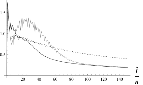
Figure 2: $L^{\infty}$ norm of the error for the optimized scheme (in black), the DRP scheme (in gray), and the FCTS scheme (dashed plot).

Figure 3 displays the $L^{2}$ norm of the error for the above optimized scheme (in black), the seventh-order DRP scheme (in gray), and the FCTS scheme (dashed plot). As expected, results coincide.

Figure 3: $L^{2}$ norm of the error for the optimized case (in black) and the optimized case (dashed curve).

5 Conclusion

The above results open new ways for the building of DRP schemes. It seems that the research on this problem has not been performed before as far as our knowledge goes. In the near future, we are going to extend the techniques described herein to nonlinear schemes, in conjunction with other innovative methods as the Lie group theory.

References

- [1] Tam, C. K. W. and Webb, J. C.(1993). Dispersion-Relation-Preserving Finite Difference Schemes for Computational Acoustics. J. of Computational Physics, 107, 262-281.
- [2] Van Dooren, P.(1984). Reduced order observers: A new algorithm and proof. Systems Control Lett., 4, 243-251.
- [3] A. Berman and Plemmons, R. J.(1994). Nonnegative Matrices in the Mathematical Sciences. SIAM, Philadelphia, PA.
- [4] Gail, H. R., Hantler, S.L. and Taylor B. A.(1996). Spectral Analysis of M/G/1 and G/M/1 type Markov chains. Adv. Appl. Probab., 28, 114-165.
- [5] Boley, D. L.(1981). Computing the Controllability algorithm / Observability Decomposition of a Linear Time-Invariant Dynamic System, A Numerical Approach. PhD. thesis, Report STAN-CS-81-860, Dept. Comp. i, Sci., Stanford University.
- [6] Deif, A. S., Seif, N. P. and Hussein, S. A.(1995). Sylvester’s equation: accuracy and computational stability. Journal of Computational and Applied Mathematics, 61, 1-11.
- [7] Hearon,J. Z.(1977). Nonsingular solutions of . Linear Algebra and its applications, 16, 57-63.
- [8] Huo, C. H.(2004). Efficient methods for solving a nonsymmetric algebraic equation arising in stochastic fluid models, Journal of Computational and Applied Mathematics, 1-21.
- [9] Tsui,C. C.(1987). A complete analytical solution to the equation and its applications. IEEE Trans. Automat. Control AC, 32, pp. 742-744.
- [10] Zhou, B. and Duan, G. R.(2005). An explicit solution to the matrix equation . Linear Algebra and its applications, 402, 345-366.
- [11] Duan, G. R.(1992). Solution to matrix equation and eigenstructure assignment for descriptor systems. Automatica, 28, 639-643.
- [12] Duan, G. R.(1996). On the solution to Sylvester matrix equation and eigenstructure assignment for descriptor systems. IEEE Trans. Automat. Control AC, 41, 276-280.
- [13] Kirrinnis, P.(2000). Fast algorithms for the Sylvester equation , Theoretical Computer Science, 259, 623-638.
- [14] Konstantinov, M., Mehrmann, V. and P. Petkov, P.(2000). On properties of Sylvester and Lyapunov operators. Linear Algebra and its applications, 312, 35-71.
- [15] Varga, A.(2003). TA numerically reliable approach to robust pole assignment for descriptor systems. Future Generation Computer Systems, 19, 1221-1230.
- [16] Witham, G. B.,(1974). Linear and Nonlinear Wave, Wiley-Interscience.
- [17] Wolfram, S.,(1999). The Mathematica book, Cambridge University Press.