A new concept of strong controllability via the Schur complement in adaptive tracking

Abstract.

We propose a new concept of strong controllability associated with the Schur complement of a suitable limiting matrix. This concept allows us to extend the previous results associated with multidimensional ARX models. On the one hand, we carry out a sharp analysis of the almost sure convergence for both least squares and weighted least squares algorithms. On the other hand, we also provide a central limit theorem and a law of iterated logarithm for these two stochastic algorithms. Our asymptotic results are illustrated by numerical simulations.

1. Introduction

Consider the $d$-dimensional autoregressive process with adaptive control of order $(p,q)$, $\mbox{ARX}_{d}(p,q)$ for short, given for all $n\geq 0$ by

(1.1) $$A(R)X_{n+1}=B(R)U_{n}+\varepsilon_{n+1}$$

where $R$ stands for the shift-back operator and $X_{n},U_{n}$ and $\varepsilon_{n}$ are the system output, input and driven noise, respectively. The polynomials $A$ and $B$ are given for all $z\in\mathbb{C}$ by

$$A(z) = I_{d}-A_{1}z-\cdots-A_{p}z^{p},$$

$$B(z) = I_{d}+B_{1}z+\cdots+B_{q}z^{q},$$

where $A_{i}$ and $B_{j}$ are unknown square matrices of order $d$ and $I_{d}$ is the identity matrix. Denote by $\theta$ the unknown parameter of the model

$$\theta^{t}=(A_{1},\ldots,A_{p},B_{1},\ldots,B_{q}).$$

Relation (1.1) can be rewritten as

(1.2) $$X_{n+1}=\theta^{t}\Phi_{n}+U_{n}+\varepsilon_{n+1}$$

where the regression vector $\Phi_{n}=\left(X_{n}^{p},U_{n-1}^{q}\right)^{t}$ with $X_{n}^{p}=(X_{n}^{t},\ldots,X_{n-p+1}^{t})$ and $U_{n}^{q}=(U_{n}^{t},\ldots,U_{n-q+1}^{t})$. In all the sequel, we shall assume the $(\varepsilon_{n})$ is a martingale difference sequence adapted to the filtration $\mathbb{F}=(\mathcal{F}_{n})$ where $\mathcal{F}_{n}$ stands for the $\sigma$-algebra of the events occurring up to time $n$. We also assume that, for all $n\geq 0$, $\mathbb{E}[\varepsilon_{n+1}\varepsilon_{n+1}^{t}|\mathcal{F}_{n}]=\Gamma$ a.s. where $\Gamma$ is a positive definite deterministic covariance matrix.

A wide literature concerning the estimation of $\theta$ as well as on the tracking control is available, [1], [4], [5], [7], [8], [10], [12], [15]. The purpose of this paper is to establish sharp asymptotic results for stochastic algorithms associated with the estimation of $\theta$ via the introduction of a new concept of strong controllability. The strong controllability is closely related to the almost sure convergence of the matrix

$$S_{n}=\sum_{k=0}^{n}\Phi_{k}\Phi_{k}^{t}.$$

In the particular case $q=0$, it was shown in [5] that

$$\lim_{n\rightarrow\infty}\frac{S_{n}}{n}=L\hskip 14.22636pt\text{a.s.}$$

where $L$ is the block diagonal matrix of order $dp$ given by

$$L=\text{diag}\left(\Gamma,\cdots,\Gamma\right).$$

Under the classical causality assumption, we shall now prove that

(1.3) $$\lim_{n\rightarrow\infty}\frac{S_{n}}{n}=\Lambda\hskip 14.22636pt\text{a.s.}$$

where $\Lambda$ is the symmetric square matrix of order $\delta=d(p+q)$

$$\Lambda=\left(\begin{array}[]{cc}L&K^{t}\\ K&H\end{array}\right)$$

and the matrices $H$ and $K$ will be explicitly calculated. It is well-known [14] that $\det(\Lambda)=\det(L)\det(S)$ where $S=H-KL^{-1}K^{t}$ is the Schur complement of $L$ in $\Lambda$. Moreover, as $L$ is positive definite, $\Lambda$ is positive definite if and only if $S$ is positive definite. Via our new concept of strong controllability, we shall propose a suitable assumption under which $S$ is positive definite. It will allow us to improve the previous results [5], [6], [10], [11] by showing a central limit theorem (CLT) and a law of iterated logarithm (LIL) for both the least squares (LS) and the weighted least squares (WLS) algorithms associated with the estimation of $\theta$.

The paper is organized as follows. Section $\!2$ is devoted to the introduction of our new concept of strong controllability together with some linear algebra calculations. Section $\!3$ deals with the parameter estimation and the adaptive control. In Section $\!4$, we establish convergence (1.3) and we deduce a CLT as well as a LIL for both LS and WLS algorithms. Some numerical simulations are provided in Section $\!5$. A short conclusion is given in Section $\!6$. All technical proofs are postponed in the Appendices.

2. Strong controllability

In all the sequel, we shall make use of the well-known causality assumption on $B$. More precisely, we assume that for all $z\in\mathbb{C}$ with $|z|\leq 1$

$({\text{A}}_1)$ $$\det(B(z))\neq 0.$$

In other words, the polynomial $\det(B(z))$ only has zeros with modulus $>1$. Consequently, if $r>1$ is strictly less than the smallest modulus of the zeros of $\det(B(z))$, then $B(z)$ is invertible in the ball with center zero and radius $r$ and $B^{-1}(z)$ is a holomorphic function (see e.g. [9] page 155). For all $z\in\mathbb{C}$ such that $|z|\leq r$, we shall denote

(2.1) $$P(z)=B^{-1}(z)(A(z)-I_{d})=\sum_{k=1}^{\infty}P_{k}z^{k}.$$

All the matrices $P_{k}$ may be explicitly calculated as functions of the matrices $A_{i}$ and $B_{j}$. For example, $P_{1}=-A_{1}$, $P_{2}=B_{1}A_{1}-A_{2}$, $P_{3}=(B_{2}-B_{1}^{2})A_{1}+B_{1}A_{2}-A_{3}$. We shall often make use of the square matrix of order $dq$ given, if $p\geq q$, by

$$\Pi=\left(\begin{array}[]{ccccc}P_{p}&P_{p+1}&\cdots&P_{p+q-2}&P_{p+q-1}\\ P_{p-1}&P_{p}&P_{p+1}&\cdots&P_{p+q-2}\\ \cdots&\cdots&\cdots&\cdots&\cdots\\ P_{p-q+2}&\cdots&P_{p-1}&P_{p}&P_{p+1}\\ P_{p-q+1}&P_{p-q+2}&\cdots&P_{p-1}&P_{p}\end{array}\right)$$

while, if $p\leq q$, by

$$\Pi=\left(\begin{array}[]{cccccc}P_{p}&P_{p+1}&\cdots&\cdots&P_{p+q-2}&P_{p+q-1}\\ \cdots&\cdots&\cdots&\cdots&\cdots&\cdots\\ P_{1}&P_{2}&\cdots&\cdots&P_{q-1}&P_{q}\\ 0&P_{1}&P_{2}&\cdots&P_{q-2}&P_{q-1}\\ \cdots&\cdots&\cdots&\cdots&\cdots&\cdots\\ 0&\cdots&0&P_{1}&\cdots&P_{p}\end{array}\right).$$

Definition 2.1.

An $\mbox{ARX}_{d}(p,q)$ is said to be strongly controllable if $B$ is causal and $\Pi$ is invertible,

$({\text{A}}_2)$ $$\det(\Pi)\neq 0.$$

Remark 2.1.

The concept of strong controllability is not really restrictive. For example, if $p=q=1$, assumption $(\text{A}_{2})$ reduces to $\det(A_{1})\neq 0$, if $p=2$, $q=1$ to $\det(A_{2}-B_{1}A_{1})\neq 0$, if $p=1$, $q=2$ to $\det(A_{1})\neq 0$, while if $p=q=2$ to

$$\det\left(\begin{array}[]{cc}A_{1}&A_{2}-B_{1}A_{1}\\ A_{2}-B_{1}A_{1}&A_{3}-B_{1}A_{2}+(B_{1}^{2}-B_{2})A_{1}\end{array}\right)\neq 0.$$

For all $1\leq i\leq q$, denote by $H_{i}$ be the square matrix of order $d$

$$H_{i}=\sum_{k=i}^{\infty}P_{k}\Gamma P_{k-i+1}^{t}.$$

In addition, let $H$ be the symmetric square matrix of order $dq$

(2.2) $$H=\left(\begin{array}[]{ccccc}H_{1}&H_{2}&\cdots&H_{q-1}&H_{q}\\ H_{2}^{t}&H_{1}&H_{2}&\cdots&H_{q-1}\\ \cdots&\cdots&\cdots&\cdots&\cdots\\ H_{q-1}^{t}&\cdots&H_{2}^{t}&H_{1}&H_{2}\\ H_{q}^{t}&H_{q-1}^{t}&\cdots&H_{2}^{t}&H_{1}\end{array}\right).$$

For all $1\leq i\leq p$, let $K_{i}=P_{i}\Gamma$ and denote by $K$ the rectangular matrix of dimension $dq\times dp$ given, if $p\geq q$, by

$$K=\left(\begin{array}[]{ccccccc}0&K_{1}&K_{2}&\cdots&\cdots&K_{p-2}&K_{p-1}\\ 0&0&K_{1}&\cdots&\cdots&K_{p-3}&K_{p-2}\\ \cdots&\cdots&\cdots&\cdots&\cdots&\cdots&\cdots\\ 0&\cdots&0&K_{1}&K_{2}&\cdots&K_{p-q+1}\\ 0&\cdots&\cdots&0&K_{1}&\cdots&K_{p-q}\end{array}\right)$$

while, if $p\leq q$, by

$$K=\left(\begin{array}[]{ccccc}0&K_{1}&\cdots&K_{p-2}&K_{p-1}\\ 0&0&K_{1}&\cdots&K_{p-2}\\ \cdots&\cdots&\cdots&\cdots&\cdots\\ 0&\cdots&0&0&K_{1}\\ 0&0&\cdots&0&0\\ \cdots&\cdots&\cdots&\cdots&\cdots\\ 0&0&\cdots&0&0\end{array}\right).$$

Finally, let $L$ be the block diagonal matrix of order $dp$

(2.3) $$L=\left(\begin{array}[]{ccccc}\Gamma&0&\cdots&0&0\\ 0&\Gamma&0&\cdots&0\\ \cdots&\cdots&\cdots&\cdots&\cdots\\ 0&\cdots&0&\Gamma&0\\ 0&0&\cdots&0&\Gamma\end{array}\right)$$

and denote by $\Lambda$ the symmetric square matrix of order $\delta=d(p+q)$

(2.4) $$\Lambda=\left(\begin{array}[]{cc}L&K^{t}\\ K&H\end{array}\right).$$

The following lemma is the keystone of all our asymptotic results.

Lemma 2.2.

Let $S$ be the Schur complement of $L$ in $\Lambda$

(2.5) $$S=H-KL^{-1}K^{t}.$$

If $(\text{A}_{1})$ and $(\text{A}_{2})$ hold, $S$ and $\Lambda$ are invertible and

(2.6) $$\Lambda^{-1}=\left(\begin{array}[]{cc}L^{-1}+L^{-1}K^{t}S^{-1}KL^{-1}&-L^{-1}K^{t}S^{-1}\\ -S^{-1}KL^{-1}&S^{-1}\end{array}\right).$$

Proof.

The proof is given in Appendix A. ∎

3. Estimation and Adaptive control

First of all, we focus our attention on the estimation of the parameter $\theta$. We shall make use of the weighted least squares (WLS) algorithm introduced by Bercu and Duflo [3], [4], which satisfies, for all $n\geq 0$,

(3.1) $$\widehat{\theta}_{n+1}=\widehat{\theta}_{n}+a_{n}S_{n}^{-1}(a)\Phi_{n}\left(X_{n+1}-U_{n}-\widehat{\theta}_{n}^{\,t}\Phi_{n}\right){\!}^{t}$$

where the initial value $\hat{\theta}_{0}$ may be arbitrarily chosen and

$$S_{n}(a)=\sum_{k=0}^{n}a_{k}\Phi_{k}\Phi_{k}^{t}+I_{\delta}$$

where the identity matrix $I_{\delta}$ with $\delta=d(p+q)$ is added in order to avoid useless invertibility assumption. The choice of the weighted sequence $(a_{n})$ is crucial. If

$$a_{n}=1$$

we find again the standard LS algorithm, while if $\gamma\!>\!0$,

$$a_{n}=\Bigl{(}\frac{1}{\log s_{n}}\Bigr{)}^{1+\gamma}\hskip 28.45274pt\text{with}\hskip 28.45274pts_{n}=\sum_{k=0}^{n}||\Phi_{k}||^{2},$$

we obtain the WLS algorithm of Bercu and Duflo.

Next, we are concern with the choice of the adaptive control $U_{n}$. The crucial role played by $U_{n}$ is to regulate the dynamic of the process $(X_{n})$ by forcing $X_{n}$ to track step by step a predictable reference trajectory $x_{n}$. We shall make use of the adaptive tracking control proposed by Astr$\ddot{\mbox{o}}$m and Wittenmark [1] given, for all $n\geq 0$, by

(3.2) $$U_{n}=x_{n+1}-\widehat{\theta}_{n}^{\,t}\,\Phi_{n}.$$

By substituting (3.2) into (1.2), we obtain the closed-loop system

(3.3) $$X_{n+1}-x_{n+1}=\pi_{n}+\varepsilon_{n+1}$$

where the prediction error $\pi_{n}=(\theta-\widehat{\theta}_{n})^{\,t}\Phi_{n}$. In all the sequel, we assume that the reference trajectory $(x_{n})$ satisfies

(3.4) $$\sum_{k=1}^{n}\parallel x_{k}\parallel^{2}=o(n)\hskip 28.45274pt\text{a.s.}$$

In addition, we also assume that the driven noise $(\varepsilon_{n})$ satisfies the strong law of large numbers which means that if

(3.5) $$\Gamma_{n}=\frac{1}{n}\sum_{k=1}^{n}\varepsilon_{k}\varepsilon_{k}^{t},$$

then $\Gamma_{n}$ converges a.s. to $\Gamma$. That is the case if, for example, $(\varepsilon_{n})$ is a white noise or if $(\varepsilon_{n})$ has a finite conditional moment of order $>2$. Finally, let $(C_{n})$ be the average cost matrix sequence defined by

$$C_{n}=\frac{1}{n}\sum_{k=1}^{n}(X_{k}-x_{k})(X_{k}-x_{k})^{t}.$$

The tracking is said to be optimal if $C_{n}$ converges a.s. to $\Gamma$.

4. Main results

Our first result concerns the almost sure properties of the LS algorithm.

Theorem 4.1.

Assume that the $\mbox{ARX}_{d}(p,q)$ model is strongly controllable and that $(\varepsilon_{n})$ has finite conditional moment of order $>2$. Then, for the LS algorithm, we have

(4.1) $$\lim_{n\rightarrow\infty}\frac{S_{n}}{n}=\Lambda\hskip 14.22636pt\text{a.s.}$$

where the limiting matrix $\Lambda$ is given by (2.4). In addition, the tracking is optimal

(4.2) $$\parallel C_{n}-\Gamma_{n}\parallel=\mathcal{O}\left(\frac{\log n}{n}\right)\hskip 14.22636pt\text{a.s.}$$

We can be more precise in (4.2) by

(4.3) $$\lim_{n\rightarrow\infty}\frac{1}{\log n}\sum_{k=1}^{n}(X_{k}-x_{k}-\varepsilon_{k})(X_{k}-x_{k}-\varepsilon_{k})^{t}=\delta\Gamma\hskip 14.22636pt\text{a.s.}$$

Finally, $\widehat{\theta}_{n}$ converges almost surely to $\theta$

(4.4) $$\parallel\widehat{\theta}_{n}-\theta\parallel^{2}=\mathcal{O}\left(\frac{\log n}{n}\right)\hskip 14.22636pt\text{a.s.}$$

Our second result is related to the almost sure properties of the WLS algorithm.

Theorem 4.2.

Assume that the $\mbox{ARX}_{d}(p,q)$ model is strongly controllable. In addition, suppose that either $(\varepsilon_{n})$ is a white noise or $(\varepsilon_{n})$ has finite conditional moment of order $>2$. Then, for the WLS algorithm, we have

(4.5) $$\lim_{n\rightarrow\infty}(\log n)^{1+\gamma}\frac{S_{n}(a)}{n}=\Lambda\hskip 14.22636pt\text{a.s.}$$

where the limiting matrix $\Lambda$ is given by (2.4). In addition, the tracking is optimal

(4.6) $$\parallel C_{n}-\Gamma_{n}\parallel=o\left(\frac{(\log n)^{1+\gamma}}{n}\right)\hskip 14.22636pt\text{a.s.}$$

Finally, $\widehat{\theta}_{n}$ converges almost surely to $\theta$

(4.7) $$\parallel\widehat{\theta}_{n}-\theta\parallel^{2}=\mathcal{O}\left(\frac{(\log n)^{1+\gamma}}{n}\right)\hskip 14.22636pt\text{a.s.}$$

Proof.

The proof is given in Appendix B. ∎

Remark 4.1.

One can observe that Theorems 4.1 and 4.2 extend the results of Bercu [5] and Guo [11] previously established in the AR framework.

Theorem 4.3.

Assume that the $\mbox{ARX}_{d}(p,q)$ model is strongly controllable and that $(\varepsilon_{n})$ has finite conditional moment of order $\alpha>2$. In addition, suppose that $(x_{n})$ has the same regularity in norm as $(\varepsilon_{n})$ which means that for all $2<\beta<\alpha$

(4.8) $$\sum_{k=1}^{n}\parallel x_{k}\parallel^{\beta}=\mathcal{O}(n)\hskip 14.22636pt\text{a.s.}$$

Then, the LS and WLS algorithms share the same central limit theorem

(4.9) $$\sqrt{n}(\widehat{\theta}_{n}-\theta)\mathrel{\mathop{\kern 0.0pt\longrightarrow}\limits^{{\mbox{\calcal L}}}}\mathcal{N}(0,\Lambda^{-1}\otimes\Gamma)$$

where the inverse matrix $\Lambda^{-1}$ is given by (2.6) and the symbol $\otimes$ stands for the matrix Kronecker product. In addition, for any vectors $u\in\mathbb{R}^{d}$ and $v\in\mathbb{R}^{\delta}$, they also share the same law of iterated logarithm

(4.10) $$\limsup_{n\rightarrow\infty}\left(\frac{n}{2\log\log n}\right)^{1/2}\!\!v^{t}(\widehat{\theta}_{n}-\theta)u = -\liminf_{n\rightarrow\infty}\left(\frac{n}{2\log\log n}\right)^{1/2}\!\!v^{t}(\widehat{\theta}_{n}-\theta)u$$

$$= \Bigl{(}v^{t}\Lambda^{-1}v\Bigr{)}^{1/2}\Bigl{(}u^{t}\Gamma u\Bigr{)}^{1/2}\hskip 14.22636pt\text{a.s.}$$

In particular,

(4.11) $$\left(\frac{\lambda_{min}\Gamma}{\lambda_{max}\Lambda}\right)\leq\limsup_{n\rightarrow\infty}\ \left(\frac{n}{2\log\log n}\right)\parallel\hat{\theta}_{n}-\theta\parallel^{2}\leq\left(\frac{\lambda_{max}\Gamma}{\lambda_{min}\Lambda}\right)\hskip 14.22636pt\text{a.s.}$$

where $\lambda_{min}\Gamma$ and $\lambda_{max}\Gamma$ are the minimum and the maximum eigenvalues of $\Gamma$.

Proof.

The proof is given in Appendix C. ∎

5. Numerical simulations

The goal of this section is to propose some numerical experiments for illustrating the asymptotic results of Section 4. In order to keep this section brief, we shall only focus our attention on a strongly controllable $ARX_{d}(p,q)$ model in dimension $d=2$ with $p=1$ and $q=1$. Our numerical simulations are based on $M=500$ realizations of sample size $N=1000$. For the sake of simplicity, the reference trajectory $(x_{n})$ is chosen to be identically zero and the driven noise $(\varepsilon_{n})$ is a Gaussian $\mathcal{N}(0,1)$ white noise. Consider the $ARX_{2}(1,1)$ model

$$X_{n+1}=AX_{n}+U_{n}+BU_{n-1}+\varepsilon_{n+1}$$

where

$$A=\left(\begin{array}[]{cc}2&0\\ 0&1\end{array}\right)\hskip 28.45274pt\text{and}\hskip 28.45274ptB=\frac{1}{4}\left(\begin{array}[]{cc}3&\,0\\ 0&\!-2\end{array}\right).$$

Figure 1 shows the almost sure convergence of the LS estimator $\widehat{\theta}_{n}$ to the four coordinates of $\theta$ which are different from zero. One can observe that $\widehat{\theta}_{n}$ performs very well in the estimation of $\theta$.

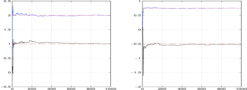
Figure 1. Left: LLN for A, Right: LLN for B.

Figure 2 shows the CLT for the four coordinates of

$$Z_{N}=\sqrt{N}\Lambda^{1/2}(\widehat{\theta}_{N}-\theta)$$

where $\Lambda$ is the limiting matrix given by (2.4) with $L=I_{2}$, $K=0$ and

$$H=A^{2}(I_{2}-B^{2})^{-1}=\frac{4}{21}\left(\begin{array}[]{cc}48&0\\ 0&7\end{array}\right).$$

One can realize that each component of $Z_{N}$ has $\mathcal{N}(0,1)$ distribution as expected.

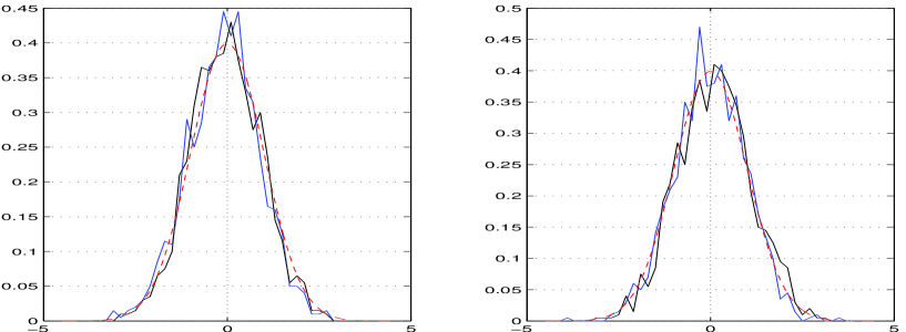
Figure 2. Left: CLT for A, Right: CLT for B.

6. Conclusion

Via our new concept of strong controllability, we have extended the analysis of the almost sure convergence for both LS and WLS algorithms in the multidimensional ARX framework. It enables us to provide a positive answer to a conjecture in [5] by establishing a CLT and a LIL for these two stochastic algorithms. In our approach, the leading matrix associated with the matrix polynomial $B$, commonly called the high frequency gain, was supposed to be known and it was chosen as the identity matrix $I_{d}$. It would be a great challenge for the control community to carry out similar analysis with unknown high frequency gain and to extend it to ARMAX models.

7. Appendix A.

Proof of Lemma 2.2. Let $\Sigma$ be the infinite-dimensional diagonal square matrix

$$\Sigma=\left(\begin{array}[]{ccccc}\Gamma&0&\cdots&\cdots&\cdots\\ 0&\Gamma&0&\cdots&\cdots\\ \cdots&0&\Gamma&0&\cdots\\ \cdots&\cdots&\cdots&\cdots&\cdots\\ \cdots&\cdots&\cdots&\cdots&\cdots\end{array}\right).$$

Moreover, denote by $T$ the infinite-dimensional rectangular matrix with $dq$ raws and an infinite number of columns given, if $p\geq q$, by

$$T=\left(\begin{array}[]{cccccc}P_{p}&P_{p+1}&\cdots&P_{k}&P_{k+1}&\cdots\\ P_{p-1}&P_{p}&\cdots&P_{k-1}&P_{k}&\cdots\\ \cdots&\cdots&\cdots&\cdots&\cdots&\cdots\\ P_{p-q+2}&P_{p-q+3}&\cdots&P_{k-q+2}&P_{k-q+3}&\cdots\\ P_{p-q+1}&P_{p-q+2}&\cdots&P_{k-q+1}&P_{k-q+2}&\cdots\end{array}\right)$$

while, if $p\leq q$, by

$$T=\left(\begin{array}[]{ccccccc}P_{p}&P_{p+1}&\cdots&\cdots&P_{k}&P_{k+1}&\cdots\\ \cdots&\cdots&\cdots&\cdots&\cdots&\cdots&\cdots\\ P_{1}&P_{2}&\cdots&\cdots&P_{k-p+1}&P_{k-p+2}&\cdots\\ 0&P_{1}&P_{2}&\cdots&P_{k-p}&P_{k-p+1}&\cdots\\ \cdots&\cdots&\cdots&\cdots&\cdots&\cdots&\cdots\\ 0&\cdots&\cdots&0&P_{1}&P_{2}&\cdots\end{array}\right).$$

After some straightforward, although rather lengthy, linear algebra calculations, it is possible to deduce from (2.5) that

(A.1) $$S=T\Sigma T^{t}.$$

It clearly follows from this suitable decomposition that

(A.2) $$\ker(S)=\ker(T^{t}).$$

As a matter of fact, assume that $v\in\mathbb{R}^{dq}$ belongs to $\ker(T^{t})$. Then, $T^{t}v=0$, $Sv=0$ which leads to $\ker(T^{t})\subset\ker(S)$. On the other hand, assume that $v\in\mathbb{R}^{dq}$ belongs to $\ker(S)$. Since $Sv=0$, we clearly have $v^{t}Sv=0$, so $v^{t}T\Sigma T^{t}v=0$. However, the matrix $\Gamma$ is positive definite. Consequently, $T^{t}v=0$ and $\ker(S)\subset\ker(T^{t})$, which implies (A.2). Moreover, it follows from the well-known rank theorem that

(A.3) $$dq=\dim(\ker(S))+\text{rank}(S).$$

As soon as $\ker(S)=\{0\}$, $\dim(\ker(S))=0$ and we obtain from (A.3) that $S$ is of full rank $dq$ which means that $S$ is invertible. Furthermore, the left hand side square matrix of order $dq$ of the infinite-dimensional matrix $T$ is precisely $\Pi$. Consequently, if $\Pi$ is invertible, $\Pi$ is of full rank $dq$, $\ker(\Pi)=\ker(\Pi^{t})=\{0\}$ and the left null space of $T$ reduces to the null vector of $\mathbb{R}^{dq}$. Hence, if $\Pi$ is invertible, we deduce from (A.2) together with (A.3) that $S$ is also invertible. Finally, as

(A.4) $$\det(\Lambda)=\det(L)\det(S)=\det(\Gamma)^{p}\det(S),$$

we obtain from (A.4) that $\Lambda$ is invertible and formula (2.6) follows from [14] page 18, which completes the proof of Lemma 2.2.$\ \ \mathbin{\vbox{\hrule\hbox{\vrule height=4.30554pt\kern 5.0pt\vrule height=4.30554pt}\hrule}}$

Appendix B.

Proof of Theorem 4.1. In order to prove Theorem 4.1, we shall make use of the same approach than Bercu [5] or Guo and Chen [10]. First of all, we recall that for all $n\geq 0$

(B.1) $$X_{n+1}-x_{n+1}=\pi_{n}+\varepsilon_{n+1}.$$

In addition, let

$$s_{n}=\sum_{k=0}^{n}||\Phi_{k}||^{2}.$$

It follows from (B.1) together with the strong law of large numbers for martingales (see e.g. Corollary 1.3.25 of [9]) that $n=\mathcal{O}(s_{n})$ a.s. Moreover, by Theorem 1 of [2] or Lemma 1 of [10], we have

(B.2) $$\sum_{k=1}^{n}(1-f_{k})\parallel\pi_{k}\parallel^{2}=\mathcal{O}(\log s_{n})\hskip 14.22636pt\text{a.s.}$$

where $f_{n}=\Phi_{n}^{t}S_{n}^{-1}\Phi_{n}$. Hence, if $(\varepsilon_{n})$ has finite conditional moment of order $\alpha>2$, we can show by the causality assumption $(\text{A}_{1})$ on the matrix polynomial $B$ together with (B.2) that $\parallel\Phi_{n}\parallel^{2}=\mathcal{O}(s_{n}^{\beta})$ a.s. for all $2\alpha^{-1}<\beta<1$. In addition, let $g_{n}=\Phi_{n}^{t}S_{n-1}^{-1}\Phi_{n}$ and $\delta_{n}=\text{tr}(S_{n-1}^{-1}-S_{n}^{-1})$. It is well-known that

$$(1-f_{n})(1+g_{n})=1$$

and $(\delta_{n})$ tends to zero a.s. Consequently, as $\parallel\pi_{n}\parallel^{2}=(1-f_{n})(1+g_{n})\parallel\pi_{n}\parallel^{2}$ and $1+g_{n}\leq 2+\delta_{n}\parallel\Phi_{n}\parallel^{2}$, we can deduce from (B.2) that

(B.3) $$\sum_{k=1}^{n}\parallel\pi_{k}\parallel^{2}=o(s_{n}^{\beta}\log s_{n})\hskip 14.22636pt\text{a.s.}$$

Therefore, we obtain from (3.4), (B.1) and (B.3) that

(B.4) $$\sum_{k=1}^{n}\parallel X_{k+1}\parallel^{2}=o(s_{n}^{\beta}\log s_{n})+\mathcal{O}(n)\hskip 14.22636pt\text{a.s.}$$

Furthermore, we infer from assumption $(\text{A}_{1})$ that

(B.5) $$U_{n}=B^{-1}(R)A(R)X_{n+1}-B^{-1}(R)\varepsilon_{n+1}$$

which implies by (B.4) that

(B.6) $$\sum_{k=1}^{n}\parallel U_{k}\parallel^{2}=o(s_{n}^{\beta}\log s_{n})+\mathcal{O}(n)\hskip 14.22636pt\text{a.s.}$$

It remains to put together the two contributions (B.4) and (B.6) to deduce that $s_{n}=o(s_{n})+\mathcal{O}(n)$ a.s. leading to $s_{n}=\mathcal{O}(n)$ a.s. Hence, it follows from (B.3) that

(B.7) $$\sum_{k=1}^{n}\parallel\pi_{k}\parallel^{2}=o(n)\hskip 14.22636pt\text{a.s.}$$

Consequently, we obtain from (3.4), (B.1) and (B.7) that

$$\lim_{n\rightarrow\infty}\frac{1}{n}\sum_{k=1}^{n}X_{k}X_{k}^{t}=\Gamma\hskip 14.22636pt\text{a.s.}\vspace{-1ex}$$

and, for all $1\leq i\leq p-1$, ${\displaystyle\sum_{k=0}^{n}X_{k}X_{k-i}^{t}}=o(n)$ a.s. which implies that

(B.8) $$\lim_{n\rightarrow\infty}\frac{1}{n}\sum_{k=1}^{n}X_{k}^{p}(X_{k}^{p})^{t}=L\hskip 14.22636pt\text{a.s.}$$

where $L$ is given by (2.3). Furthermore, it follows from relation (1.1) together with (B.1) and assumption $(\text{A}_{1})$ that, for all $n\geq 0$,

$$U_{n} = B^{-1}(R)A(R)X_{n+1}-B^{-1}(R)\varepsilon_{n+1},$$

$$= B^{-1}(R)A(R)(\pi_{n}+x_{n+1})+B^{-1}(R)(A(R)-I_{d})\varepsilon_{n+1},$$

$$= V_{n}+W_{n+1}.$$

Consequently, as $W_{n}=P(R)\varepsilon_{n}$, we deduce from (3.4), (B.7) and the strong law of large numbers for martingales (see e.g. Theorem 4.3.16 of [9]) that, for all $1\leq i\leq q$,

$$\lim_{n\rightarrow\infty}\frac{1}{n}\sum_{k=1}^{n}U_{k}U_{k-i+1}^{t}=H_{i}\hskip 14.22636pt\text{a.s.}$$

which ensures that

(B.9) $$\lim_{n\rightarrow\infty}\frac{1}{n}\sum_{k=1}^{n}U_{k}^{q}(U_{k}^{q})^{t}=H\hskip 14.22636pt\text{a.s.}$$

where $H$ is given by (2.2). Via the same lines, we also find that

(B.10) $$\lim_{n\rightarrow\infty}\frac{1}{n}\sum_{k=1}^{n}X_{k}^{p}(U_{k-1}^{q})^{t}=K^{t}\hskip 14.22636pt\text{a.s.}$$

Therefore, it follows from the conjunction of (B.8), (B.9) and (B.10) that

(B.11) $$\lim_{n\rightarrow\infty}\frac{S_{n}}{n}=\Lambda\hskip 14.22636pt\text{a.s.}$$

where the limiting matrix $\Lambda$ is given by (2.4). Hereafter, we recall that the $\mbox{ARX}_{d}(p,q)$ model is strongly controllable. Thanks to Lemma 2.2, the matrix $\Lambda$ is invertible and $\Lambda^{-1}$, given by (2.6), may be explicitly calculated. This is the key point for the rest of the proof. On the one hand, it follows from (B.11) that $n=\mathcal{O}(\lambda_{min}(S_{n}))$, $\parallel\Phi_{n}\parallel^{2}=o(n)$ a.s. which implies that $f_{n}$ tends to zero a.s. Hence, by (B.2), we find that

(B.12) $$\sum_{k=1}^{n}\parallel\pi_{k}\parallel^{2}=\mathcal{O}(\log n)\hskip 14.22636pt\text{a.s.}$$

On the other hand, we obviously have from (B.1)

(B.13) $$\parallel C_{n}-\Gamma_{n}\parallel=\mathcal{O}\left(\frac{1}{n}\sum_{k=1}^{n}\parallel\pi_{k-1}\parallel^{2}\right)\hskip 14.22636pt\text{a.s.}$$

Consequently, we immediately obtain the tracking optimality (4.2) from (B.12) and (B.13). Furthermore, by a well-known result of Lai and Wei [15] on the LS estimator, we also have

(B.14) $$\parallel\widehat{\theta}_{n+1}-\theta\parallel^{2}=\mathcal{O}\left(\frac{\log\lambda_{max}S_{n}}{\lambda_{min}S_{n}}\right)\hskip 14.22636pt\text{a.s.}$$

Hence (4.4) clearly follows from (B.11) and (B.14). Moreover, we also infer from Lemma 1 of Wei [17] together with (B.11) that

(B.15) $$(\widehat{\theta}_{n+1}-\theta)^{t}S_{n}(\widehat{\theta}_{n+1}-\theta)=o(\log n)\hskip 14.22636pt\text{a.s.}\vspace{1ex}$$

However, it follows from Theorem 4.3.16 part 4 of [9] that

(B.16) $$\lim_{n\rightarrow\infty}\frac{1}{\log d_{n}}\left((\widehat{\theta}_{n+1}-\theta)^{t}S_{n}(\widehat{\theta}_{n+1}-\theta)+\sum_{k=0}^{n}(1-f_{k})\pi_{k}\pi_{k}^{t}\right)=\Gamma\hskip 14.22636pt\text{a.s.}$$

where $d_{n}=det(S_{n})$. In addition, if $\delta=d(p+q)$, we deduce from (B.11) that

(B.17) $$\lim_{n\rightarrow\infty}\frac{d_{n}}{n^{\delta}}=\det\Lambda\hskip 14.22636pt\text{a.s.}$$

Finally, (B.15) together with (B.16) and (B.17) imply (4.3), which achieves the proof of Theorem 4.1. $\ \ \mathbin{\vbox{\hrule\hbox{\vrule height=4.30554pt\kern 5.0pt\vrule height=4.30554pt}\hrule}}$

Proof of Theorem 4.2. By Theorem 1 of [4], we have

(B.18) $$\sum_{n=1}^{\infty}a_{n}(1-f_{n}(a))\parallel\pi_{n}\parallel^{2}<+\infty\hskip 14.22636pt\text{a.s.}$$

where $f_{n}(a)=a_{n}\Phi_{n}^{t}S_{n}^{-1}(a)\Phi_{n}$. Then, as $a_{n}^{-1}=(\log(s_{n}))^{1+\gamma}$ with $\gamma>0$, we clearly have $a_{n}^{-1}=\mathcal{O}(s_{n})$ a.s. Hence, it follows from (B.18) together with Kronecker’s Lemma given e.g. by Lemma 1.3.14 of [9] that

(B.19) $$\sum_{k=1}^{n}\parallel\pi_{k}\parallel^{2}=o(s_{n})\hskip 14.22636pt\text{a.s.}$$

Therefore, we obtain from (3.4), (B.1) and (B.19) that

(B.20) $$\sum_{k=1}^{n}\parallel X_{k+1}\parallel^{2}=o(s_{n})+\mathcal{O}(n)\hskip 14.22636pt\text{a.s.}$$

In addition, we also deduce from assumption $(\text{A}_{1})$ that

(B.21) $$\sum_{k=1}^{n}\parallel U_{k}\parallel^{2}=o(s_{n})+\mathcal{O}(n)\hskip 14.22636pt\text{a.s.}$$

Consequently, we immediately infer from (B.20) and (B.21) that $s_{n}=o(s_{n})+\mathcal{O}(n)$ so $s_{n}=\mathcal{O}(n)$ a.s. Hence, (B.19) implies that

(B.22) $$\sum_{k=1}^{n}\parallel\pi_{k}\parallel^{2}=o(n)\hskip 14.22636pt\text{a.s.}$$

Proceeding exactly as in Appendix A, we find from (B.22) that

$$\lim_{n\rightarrow\infty}\frac{S_{n}}{n}=\Lambda\hskip 14.22636pt\text{a.s.}$$

Via an Abel transform, it ensures that

(B.23) $$\lim_{n\rightarrow\infty}(\log n)^{1+\gamma}\frac{S_{n}(a)}{n}=\Lambda\hskip 14.22636pt\text{a.s.}$$

We obviously have from (B.23) that $f_{n}(a)$ tends to zero a.s. Consequently, we obtain from (B.18) and Kronecker’s Lemma that

(B.24) $$\sum_{k=1}^{n}\parallel\pi_{k}\parallel^{2}=o((\log s_{n})^{1+\gamma})\hskip 14.22636pt\text{a.s.}$$

Then, (4.6) clearly follows from (B.13) and (B.24). Finally, by Theorem 1 of [4]

(B.25) $$\parallel\widehat{\theta}_{n+1}-\theta\parallel^{2}=\mathcal{O}\left(\frac{1}{\lambda_{min}S_{n}(a)}\right)\hskip 14.22636pt\text{a.s.}$$

Hence, we obtain (4.7) from (B.23) and (B.25), which completes the proof of Theorem 4.2. $\ \ \mathbin{\vbox{\hrule\hbox{\vrule height=4.30554pt\kern 5.0pt\vrule height=4.30554pt}\hrule}}$

Appendix C.

Proof of Theorem 4.3. First of all, it follows from (1.2) together with (3.1) that, for all $n\geq 1$,

(C.1) $$\widehat{\theta}_{n}-\theta=S_{n-1}^{-1}(a)M_{n}(a)$$

where

(C.2) $$M_{n}(a)=\widehat{\theta}_{0}-\theta+\sum_{k=1}^{n}a_{k-1}\Phi_{k-1}\varepsilon_{k}^{t}.$$

We now make use of the CLT for multivariate martingales given e.g. by Lemma C.1 of [5], see also [9], [13]. On the one hand, for the LS algorithm, we clearly deduce (4.9) from convergence (4.1) and decomposition (C.1). On the other hand, for the WLS algorithm, we also infer (4.9) from convergence (4.5) and (C.1). Next, we make use of the LIL for multivariate martingales given e.g. by Lemma C.2 of [5], see also [9], [16]. For the LS algorithm, since $(\varepsilon_{n})$ has finite conditional moment of order $\alpha>2$, we obtain from Chow’s Lemma given e.g. by Corollary 2.8.5 of [16] that, for all $2<\beta<\alpha$,

(C.3) $$\sum_{k=1}^{n}\parallel\varepsilon_{k}\parallel^{\beta}=\mathcal{O}(n)\hskip 14.22636pt\text{a.s.}$$

Consequently, as the reference trajectory $(x_{n})$ satisfies (4.8), we deduce from (B.1) together with (B.12) and (C.3) that

(C.4) $$\sum_{k=1}^{n}\parallel X_{k}\parallel^{\beta}=\mathcal{O}(n)\hskip 14.22636pt\text{a.s.}$$

Furthermore, it follows from (B.5) and (C.4) that

(C.5) $$\sum_{k=1}^{n}\parallel U_{k}\parallel^{\beta}=\mathcal{O}(n)\hskip 14.22636pt\text{a.s.}$$

Hence, we clearly obtain from (C.4) and (C.5) that

(C.6) $$\sum_{k=1}^{n}\parallel\Phi_{k}\parallel^{\beta}=\mathcal{O}(n)\hskip 14.22636pt\text{a.s.}$$

Therefore, as $\beta>2$, (C.6) immediately implies that

$$\sum_{n=1}^{\infty}\left(\frac{\parallel\Phi_{n}\parallel}{\sqrt{n}}\right)^{\beta}<+\infty\hskip 14.22636pt\text{a.s.}$$

Finally, Lemma C.2 of [5] together with convergence (4.1) and (C.1) lead to (4.10). The proof for the WLS algorithm is left to the reader because it follows essentially the same arguments than the proof for the LS algorithm. It is only necessary to add the weighted sequence $(a_{n})$ and to make use of convergence (4.5).$\ \ \mathbin{\vbox{\hrule\hbox{\vrule height=4.30554pt\kern 5.0pt\vrule height=4.30554pt}\hrule}}$

References

- [1] K. J. Aström and B. Wittenmark, Adaptive Control, 2nd edition, Addison-Wesley, New York, 1995.
- [2] B. Bercu, Sur l’estimateur des moindres carrés généralisés d’un modèle ARMAX. Application à l’identification des modèles ARMA. Annales de l’Institut Henri Poincaré, 27, (1991), pp. 425-443.
- [3] B. Bercu and M. Duflo, Moindres carrés pondérés et poursuite, Annals de l’Institut Henri Poincaré, 28 (1992), pp. 403-430.
- [4] B. Bercu, Weighted estimation and tracking for ARMAX models, SIAM J. Control Optim., 33 (1995), pp. 89-106.
- [5] B. Bercu, Central limit theorem and law of iterated logarithm for least squares algorithms in adaptive tracking, SIAM J. Control Optim., 36 (1998), pp. 910-928.
- [6] B. Bercu and B. Portier, Adaptive control of parametric nonlinear autoregressive models via a new martingale approach, IEEE Trans. Automat. Control, 47, (2002), pp. 1524-1528.
- [7] P. E. Caines, Linear Stochastic Systems, John Wiley, New York, 1988.
- [8] H. F. Chen and L. Guo, Identification and Stochastic Adaptive Control, Birkhäuser, Boston, 1991.
- [9] M. Duflo, Random Iterative Models, Springer Verlag, Berlin, 1997.
- [10] L. Guo and H. F. Chen, The Aström Wittenmark self-tuning regulator revisited and ELS-based adaptive trackers, IEEE Trans. Automat. Control, 36 (1991), pp. 802-812.
- [11] L. Guo, Further results on least squares based adaptive minimum variance control, SIAM J. Control Optim., 32 (1994), pp. 187-212.
- [12] L. Guo, Self convergence of weighted least squares with applications to stochastic adaptive control, IEEE Trans. Automat. Control, 41 (1996), pp. 79-89.
- [13] P. Hall and C. C. Heyde, Martingale limit theory and its application, Academic Press, New York, 1980.
- [14] R. A. Horn and C. R. Johnson, Matrix Analysis, Cambridge University Press, New York, 1990.
- [15] T. L. Lai and C. Z. Wei, Extended least squares and their applications to adaptive control and prediction in linear systems, IEEE Trans. Automat. Control, 31 (1986), pp. 898-906.
- [16] W. F. Stout, Almost sure convergence, Academic Press, New York, 1974.
- [17] C. Z. Wei, Adaptive prediction by least squares predictors in stochastic regression models with applications to time series, Annals of Statistics, 15 (1987), pp. 1667-1682.