A blind test of photometric redshifts on ground-based data

Abstract

Aims. Several photometric redshift (photo-$z$) codes are discussed in the literature and some are publicly available to be used by the community. We analyse the relative performance of different codes in blind applications to ground-based data. In particular, we study how the choice of the code-template combination, the depth of the data, and the filter set influences the photo-$z$ accuracy.

Methods. We performed a blind test of different photo-$z$ codes on imaging datasets with different depths and filter coverages and compared the results to large spectroscopic catalogues. We analysed the photo-$z$ error behaviour to select cleaner subsamples with more secure photo-$z$ estimates. We consider Hyperz, BPZ, and the code used in the CADIS, COMBO-17, and HIROCS surveys.

Results. The photo-$z$ error estimates of the three codes do not correlate tightly with the accuracy of the photo-$z$’s. While very large errors sometimes indicate a true catastrophic photo-$z$ failure, smaller errors are usually not meaningful. For any given dataset, we find significant differences in redshift accuracy and outlier rates between the different codes when compared to spectroscopic redshifts. However, different codes excel in different regimes. The agreement between different sets of photo-$z$’s is better for the subsample with secure spectroscopic redshifts than for the whole catalogue. Outlier rates in the latter are typically larger by at least a factor of two.

Conclusions. Running today’s photo-$z$ codes on well-calibrated ground-based data can lead to reasonable accuracy. The actual performance on a given dataset is largely dependent on the template choice and on realistic instrumental response curves. The photo-$z$ error estimation of today’s codes from the probability density function is not reliable, and reported errors do not correlate tightly with accuracy. It would be desirable to improve this aspect for future applications so as to get a better handle on rejecting objects with grossly inaccurate photo-$z$’s. The secure spectroscopic subsamples commonly used for assessments of photo-$z$ accuracy may be biased toward objects for which the photo-$z$’s are easier to estimate than for a complete flux-limited sample, resulting in very optimistic estimates.

1 Introduction

Photometric redshifts (hereafter, photo-$z$) have become a standard tool for the observing astronomer in the last years (Loh & Spillar 1986; Connolly et al. 1995; Koo 1999; Wolf et al. 1999; Benítez 2000; Bolzonella et al. 2000; Richards et al. 2001; Budavári et al. 2001; Wolf et al. 2001; Csabai et al. 2003; Firth et al. 2003; Collister & Lahav 2004; Babbedge et al. 2004; Ilbert et al. 2006; Feldmann et al. 2006). Not only are large multi-colour imaging surveys planned and executed with the goal of estimating the redshift of as many galaxies as possible from their broad-band photometry, but also many smaller projects benefit from this technique by providing redshifts that are much cheaper, in terms of telescope time, than spectroscopic ones and may go deeper.

Users of photo-$z$’s are often concerned with three main performance issues, which are the mean redshift error, the rate of catastrophic failures, and the validity of the probability density function (PDF) in a frequentist interpretation. The PDF may be correct in a Bayesian interpretation when including systematic uncertainties in the model fitting and correctly express a degree of uncertainty. However, given the non-statistical nature of systematic uncertainties a frequentist PDF that correctly describes the redshift distribution in the real experiment is necessarily different, unless such systematics can be excluded.

The process depends on three ingredients: model, classifier, and data. A basic issue at the heart of problems with the PDF are the match between data and model, since best-fitting parameters and confidence intervals in $\chi^{2}$-fitting are only reliable when the model is appropriate. The importance in choosing the type of data is the need to break degeneracies between ambiguous model interpretations. Finally, the classifiers are expected to produce similar results, while they could produce them at dramatically different speed. Artificial Neural Nets, hereafter ANNs, are especially fast once training has been accomplished (Firth et al. 2003).

There are many cases in the literature where the precision of photo-$z$’s has been improved after recalibrating the match between data and model (see e.g. Csabai et al. 2003; Benítez et al. 2004; Ilbert et al. 2006; Coe et al. 2006; Capak et al. 2007), although this process requires a large, representative training set of spectroscopic redshifts from the pool of data that is to be photo-$z$’ed. If ANNs are trained with sufficiently large training samples they can achieve the highest accuracies within the training range as a mismatch between data and model is ruled out from the start.

The literature reports several different photo-$z$ estimators in use across the community, some of which use different template models and some of which allow implementation of user-defined template sets. Assuming a modular problem, where model (templates), classifier, and data can be interchanged, it is interesting to test how comparable the results of different combinations are. In this spirit, we have started the work presented in this paper, where we analyse photo-$z$ performance from real ground-based survey data, in dependence of magnitude, depth of data, filter coverage, redshift region, and choice of photo-$z$ code. We concentrate on the blind performance of photo-$z$’s which is the most important benchmark for any study that cannot rely on recalibration, e.g. in the absence of spectroscopic redshifts. We choose to focus on ground-based datasets because a lot of codes were tested on the Hubble-Deep-Field for which results can already be found in the literature (see e.g. Hogg et al. 1998; Bolzonella et al. 2000; Benítez 2000).

Meanwhile, a much larger initiative has formed to investigate all (even subtle) differences in workings and outcomes among codes and models. This initiative called PHAT (PHoto-$z$ Accuracy Testing) engages a world-wide community of photo-$z$ developers and users and will hopefully develop our understanding of photo-$z$’s to a reliably predictive level.

The paper is organised as follows. In Sect. 2 the imaging and spectroscopic datasets are presented. The photo-$z$ codes used for this study are described in Sect. 3. Sect. 4 presents our approach for describing photo-$z$ accuracy. The results are presented and discussed in Sect. 5. The different photo-$z$ estimates are compared to each other in Sect. 6. A final summary and general conclusions are given in Sect. 7.

Throughout this paper we use Vega magnitudes if not otherwise mentioned.

2 Datasets

We investigate the performance of photo-$z$’s on three different imaging datasets:

1. We use five-colour $UBVRI$ data from the ESO Deep Public Survey (DPS) field Deep2c centred on the Chandra Deep Field South (CDFS) which were observed with the Wide Field Imager (WFI) at the 2.2m telescope at La Silla, Chile, reduced with the THELI reduction pipeline, and described in detail in Hildebrandt et al. (2006) as part of the Garching-Bonn Deep Survey (GaBoDS). The data originate from different projects, mostly from the ESO Imaging Survey (EIS), the COMBO-17 survey, and the GOODS program. Results for these data can be regarded as representative for very deep ground-based, wide-field surveys with the typical photometric accuracy achievable for multi-chip camera, multi-epoch data.

   In order to measure unbiased object colours the $BVRI$ images were filtered to the seeing of the $U$-band ($\approx 1\aas@@fstack{\prime\prime}0$) and the photometric catalogue was created with SExtractor (Bertin & Arnouts 1996) in dual-image-mode with the unfiltered $R$-band image as the detection image.

2. On the same field and taken with the same camera there are catalogues available from the COMBO-17 survey covering the same broad-band filters in $BVRI$ to considerably shallower depth, a different $U$-band filter, and 12 additional medium-band filters in the optical wavelength range. These data are described in detail in Wolf et al. (2004). In terms of exposure time the COMBO images are shallower by a factor of 2.5 ($R$-band) to 12.5 ($V$-band) corresponding to approximately 0.4-1.7 magnitudes.

   The broad-band data from COMBO-17 resemble a medium-deep wide-field survey, while the full 17-filter data are presently unique in its kind. However, we can use them to investigate whether additional telescope time should be spent on increasing depth as in GaBoDS or on obtaining additional SED information as in COMBO-17.

   In contrast to GaBoDS, the COMBO-17 photometry was measured directly on unfiltered images. The photometry was obtained in Gaussian apertures whose width was adapted to compensate seeing variations between the frames. Provided the convolution of aperture and PSF yields the same result for each frame, this procedure is mathematically identical to filtering all frames to a final constant seeing and extracting fluxes with Gaussian apertures at the end.

   The calibration of the CDFS field of COMBO-17 has however changed since the original publication of the data in 2004. COMBO-17 is calibrated by two spectrophotometric standard stars in each of its fields. However, the two stars on the CDFS suggested calibrations that were inconsistent in colour at the 0.15 mag level from $B$ to $I$. Both were marginally consistent with the colours of the Pickles atlas, so the choice was unconstrained. Wolf et al. (2004) ended up trusting the wrong star and introducing a colour bias towards the blue. The calibration has since been changed to follow the other star, and is now consistent with both the GaBoDS and MUSYC (Multiwavelength Survey by Yale-Chile) calibration. The consequences of the calibration change for the photo-$z$’s is little in the 17-filter case, but large when only using broad bands. Broad-band photo-$z$’s hinge more on colours than on features that are traced in medium-band photo-$z$’s.

3. Furthermore, we use catalogues from the FORS Deep Field (FDF; see Heidt et al. 2003; Gabasch 2004) involving eight broad-band filters, $UBgRIZJK_{s}$, observed with FORS@VLT in the optical and SOFI@NTT in the near-infrared. At least in the optical, these data are representative of very deep pencil-beam surveys achievable with present day large telescopes. With this dataset we are able to quantify the impact of adding near-infrared data to deep optical data on photo-$z$’s. The FDF photometric catalogue contains flux measurements in apertures of different sizes obtained after filtering images to the same PSF. In the following, we use fluxes in aperture diameters of $d=1\aas@@fstack{\prime\prime}5$ .

2.1 Comparisons of imaging data

In all three datasets, the multi-band fluxes of a given object were effectively measured in identical physical apertures outside the atmosphere (and with identical spatial weighting) for all filters, assuming that seeing produces a Gaussian-shaped PSF. Colours could still be biased by non-Gaussianity of the PSF and by suboptimal background subtraction.

The properties of these three imaging datasets are summarised in Table 1. Since the limiting magnitudes are estimated in completely different ways in the three data release papers, we decided to calculate hypothetical 10$\sigma$ limiting magnitudes with the GaBoDS values as a reference. These $m_{\mathrm{lim,eff}}$ correspond to the 10$\sigma$ sky noise under the following assumption:

$$m_{\mathrm{lim,eff,X}}-m_{\mathrm{lim,G}}=-2.5\log\left(\frac{\mathrm{FWHM_{\mathrm{X}}}}{\mathrm{FWHM_{\mathrm{G}}}}\right)\sqrt{\frac{t_{\mathrm{exp,G}}}{t_{\mathrm{exp,X}}}}\left(\frac{2.2\leavevmode\nobreak\ {\rm m}}{D}\right)\,,$$ (1)

with $\mathrm{G}$ denoting GaBoDS quantities and $\mathrm{X}$ denoting quantities of the other dataset. FWHM is the measured seeing, $t_{\mathrm{exp}}$ is the exposure time, and $D$ is the diameter of the telescope. By doing so we neglect differences between similar filter transmission curves and variations in observing conditions (moon, sky transparency etc.) Thus, the limiting magnitudes are only rough estimates for approximate comparison.

The FDF limiting magnitudes in the $ZJKs$-bands are the ones given in Heidt et al. (2003) and Gabasch (2004) corresponding to 50% completeness.

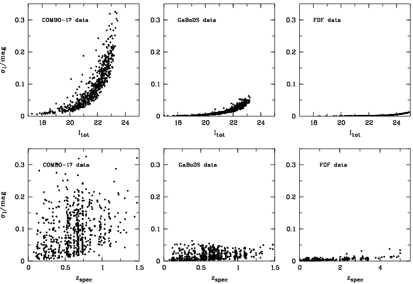
The dependence of photometric errors on magnitude and redshift in the three datasets is shown in Fig. 1. The errors for the COMBO data are derived from multiple measurements of the same sources, where photon shot-noise is assumed to be a lower limit. The GaBoDS and FDF errors are purely derived from shot-noise as no multiple measurements were made.

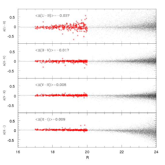
We compare the colour measurements in the COMBO and the GaBoDS catalogue and find very good agreement (see Fig. 2). Thus, the different ways of correcting for the PSF variations from band to band deliver consistent results. We carried out another comparison between the COMBO data and the CDFS catalogue from the MUSYC collaboration (E. Taylor, private communication) and the agreement is similar. We conclude that the colour measurement cannot be a dominant source of systematic error in the following.

Table 1: Properties of the imaging data.

	COMBO-17			GaBoDS			FDF
Band	Exp. time	FWHM	$m_{\mathrm{lim,eff}}$ [mag]	Exp. time	FWHM	$m_{\mathrm{lim}}$ [mag]	Exp. time	FWHM	$m_{\mathrm{lim,eff}}$ [mag]b
	[s]		10$\sigma$ sky noise	[s]		10$\sigma$ sky noise	[s]		10$\sigma$ sky noise
$U$	$21\,600$	$1\aas@@fstack{\prime\prime}00$	24.6	$78\,900$	$1\aas@@fstack{\prime\prime}01$	25.3	$44\,400$	$0\aas@@fstack{\prime\prime}97$	26.4
$B$	$11\,240$	$1\aas@@fstack{\prime\prime}10$	26.2	$69\,400$	$0\aas@@fstack{\prime\prime}98$	27.3	$22\,700$	$0\aas@@fstack{\prime\prime}60$	28.6
$V/g$	$8400$	$1\aas@@fstack{\prime\prime}20$	25.2	$104\,600$	$0\aas@@fstack{\prime\prime}92$	26.9	$22\,100$	$0\aas@@fstack{\prime\prime}87$	27.5
$R$	$35\,700$	$0\aas@@fstack{\prime\prime}75$	26.4	$87\,700$	$0\aas@@fstack{\prime\prime}79$	26.8	$26\,400$	$0\aas@@fstack{\prime\prime}75$	27.6
$I$	$9800$	$1\aas@@fstack{\prime\prime}20$	23.6	$34\,600$	$0\aas@@fstack{\prime\prime}93$	24.6	$24\,900$	$0\aas@@fstack{\prime\prime}53$	26.4
$Z$	-	-	-	-	-	-	$18\,000$	$0\aas@@fstack{\prime\prime}48$	25.3
$J$	-	-	-	-	-	-	4800	$1\aas@@fstack{\prime\prime}20$	22.9
$K_{s}$	-	-	-	-	-	-	4800	$1\aas@@fstack{\prime\prime}24$	20.7

Figure 1: Photometric errors in the $I$-band as a function of $I$-magnitude (upper panel) and as a function of spectroscopic redshift (lower panel) for the COMBO-17 data (left), the GaBoDS data (middle), and the FDF data (right); see text for information on how the errors were estimated. Note that the errors of the photometric zeropoints are larger than the purely statistical errors plotted here.

Figure 2: Comparison of colour measurements for objects in the GaBoDS and the COMBO catalogues. Note that the $U$-band filters in the two datasets are different, with the GaBoDS filter being broader and bluer. The star symbols represent objects selected by the SExtractor CLASS_STAR parameter in the magnitude range $17<R<20$.

2.2 Spectroscopic catalogues

Spectroscopic catalogues are publicly available for both fields:

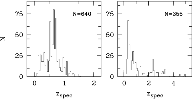
1. The VIMOS VLT Deep Survey (VVDS) team carried out an $I_{AB}<24$ magnitude limited spectroscopic survey on the CDFS with VIMOS@VLT (Le Fèvre et al. 2004) yielding 1599 redshifts including 1452 galaxies. The redshift measurements have associated reliability flags, and in the following comparisons we use only objects with flags 3 or 4 (or secondary targets with flags 23 or 24) indicating 95% and 100% confidence, respectively, to avoid errors introduced by the spectroscopic catalogue. This leaves us with 640 objects with $R_{\mathrm{WFI}}<24$, whose redshift distribution is shown in Fig. 3. Since there are very few objects beyond redshift $z\approx 1.2$ this catalogue is ideally suited to assess the performance of photo-$z$’s with optical data alone.

2. The FDF team measured the redshifts of 355 objects with FORS@VLT (341 of which are published in Noll et al. 2004) pre-selected by photo-$z$’s to cover the range $0<z<5$. The spectroscopic redshift distribution is also shown in Fig. 3 in comparison to the one of the VVDS data. This deep dataset extends well beyond the region where optical photo-$z$’s work well and can illustrate the benefit of near-infrared data on photo-$z$ performance for $z>1$.

Figure 3: Spectroscopic redshift distributions of the comparison samples. Left: The VVDS-CDFS spectroscopic data with $R_{\mathrm{WFI}}<24$ and flags 3,4,23,24. Right: The FDF spectroscopic data.

3 Photo-$z$ codes

There are basically two different approaches to estimate a photo-$z$ for a galaxy, the “SED-fitting”-method and the “empirical training set”-method. The former relies on a sample of synthetic or observed spectral-energy-distributions (SEDs) and on theoretical knowledge how those SEDs evolve with redshift. The latter relies on a colour catalogue of spectroscopically observed galaxies as large as possible to cover essentially every galaxy type at all redshifts. See e.g. Benítez (2000) for a detailed review of both techniques and their differences.

The empirical approach can lead to very precise results if an extensive, complete spectroscopic catalogue with colour information is available. But it is not as flexible as the “SED-fitting” method because for every new filter set or camera the colour catalogue must be recreated. Moreover, it is essentially limited to the magnitude range where spectra are available in large numbers ($I\la 24$) and implicit priors are driven by the spectroscopic sample selection.

The “SED-fitting”-method, however, can be applied to every dataset for which the filter transmission curves are known. Since we want to give guidance for blind applications of photo-$z$’s here we concentrate on this approach in the following.

In practise, a photo-$z$ analysis often involves aspects from both approaches. Empirical colour-redshift relations can certainly be extrapolated in magnitude or redshift. Also, a spectroscopic catalogue can help to optimise parts of an “SED-fitting” approach. Ilbert et al. (2006), e.g., present a method to improve the photo-$z$ estimates in the CFHT Legacy Survey. They adjust the photometric zeropoints of their images and optimise the template SEDs with help of more than 3000 spectroscopically observed galaxies in the range $0<z<5$. The optimisation of templates was already used for improving template based photo-$z$ estimates in the SDSS (Csabai et al. 2003). Gabasch et al. (2004) claim to obtain highly accurate photo-$z$’s in the FDF by constructing semi-empirical template SEDs from 280 spectroscopically observed galaxies in the FDF and the Hubble Deep Field. In the following we describe the three codes used for this study.

3.1 Hyperz

The “SED-fitting” photo-$z$ code Hyperz (Bolzonella et al. 2000) is publicly available, well documented and widely used by the community. For detailed information on the code see the manual at the website or the reference paper mentioned above.

Hyperz comes with two different template SED sets, the mean observed spectra of local galaxies by Coleman et al. (1980), hereafter CWW, and synthetic spectra created from the spectral evolution library of Bruzual & Charlot (1993), hereafter BC. We use the BC templates for Hyperz since for all tested setups performance with the CWW templates is worse. Different reddening laws are implemented to account for the effect of interstellar dust on the spectral shape. By default we use the reddening law of Calzetti et al. (2000) derived for local star-forming galaxies. The damping of the Lyman-$\alpha$-forest increasing with redshift is modelled according to Madau (1995). Another important option influencing performance strongly is the application of a prior on the absolute magnitude. For a given cosmology the absolute magnitude of an object is calculated from the apparent magnitude in a reference filter for every redshift step. The user can specify limits to exclude unrealistically bright or faint objects. In the following we assume a $\Lambda$CDM cosmology ($\Omega_{\Lambda}=0.7$, $\Omega_{\mathrm{m}}=0.3$, $H_{0}=70\mathrm{\frac{km}{s\cdot Mpc}}$) and allow galaxies to have an absolute $I$-band magnitude of $M_{*}-2.5<I_{\mathrm{abs}}<M_{*}+2.5$ using the local SDSS-value of $M_{*,\mathrm{AB}}=-21.26$ from Blanton et al. (2001).

Besides reporting the most probable redshift estimate as a primary solution Hyperz can also store the redshift probability distribution giving the probability associated with the $\chi^{2}$-value for every redshift step. Furthermore, the width of this distribution around the primary solution is provides a confidence interval, which allows the user to identify objects with very uncertain estimates.

We choose a minimum photometric error of 0.1mag for Hyperz to avoid unrealistically small errors in some of the bands.

3.2 COMBO-17 code

The photo-$z$ code of COMBO-17 (also used for CADIS and HIROCS; “COMBO code” hereafter) performs two simultaneous tasks: it classifies objects into stars, galaxies, QSOs, and white dwarfs based on their colours, and for galaxies and QSOs it also estimates redshifts. Here, we used a setup forcing the galaxy interpretation in order to better compare the results to the other codes which assume a priori that all objects are galaxies. The code is currently not publicly available.

It uses a 2D age $\times$ extinction grid of templates produced with the PEGASE population synthesis code (Fioc & Rocca-Volmerange 1997) and an external SMC reddening law. For all template details we refer the reader to Wolf et al. (2004). No explicit redshift-dependent prior is used, however, for the shallow purely optical datasets of COMBO-17 and GaBoDS, only galaxy redshifts up to 1.4 are considered, while for the FDF dataset the whole range from $z=0$ to $z=7$ is allowed.

The SED fitting is done in colour space rather than in magnitude space. Similar to Hyperz a lower error threshold is applied (0.05mag) but here for the colour indices.

The code determines the redshift probability distribution $p(z)$ and reports the mean of this distribution as a Minimum-Error-Variance (MEV) redshift and its RMS as an error estimate. The code also tests the shape of $p(z)$ for bimodality, and determines redshift and error from the mode with the higher integral probability (for all details see Wolf et al. 2001).

3.3 BPZ

BPZ (Bayesian photo-$z$’s) is a public code, which implements the method described in Benítez (2000). It is an SED fitting method combined with a redshift/type prior, $p(z,T|m)$, which depends on the observed magnitude of the galaxies. It originally used a set of 6 templates formed by the 4 CWW set and two starburst templates from Kinney et al. (1996) which were shown to significantly improve the photo-$z$ estimation. It should be stressed that the extrapolation to the UV and IR of the optical CWW templates used by BPZ is quite different from the one used by Hyperz. The template library has been calibrated using a set of HST and other ground based observations as described in Benítez et al. (2004). This template set has been shown to remarkably well represent the colours of galaxies in HST observations, to the point of being able to photometrically calibrate the NIC3 Hubble UDF observations with a 0.03 magnitude error as shown in Coe et al. (2006). In the latter paper two additional, very blue templates from the Bruzual & Charlot library were introduced, so the current BPZ library contains 8 templates.

The redshift likelihood is calculated by BPZ in a similar way as by Hyperz minimising the $\chi^{2}$ of observed and predicted colours. However, in contrast to Hyperz no reddening is applied to the templates relying on the completeness of the given set. After the calculation of the likelihood, Bayes theorem is applied incorporating the prior probability. The actual shape of this prior is dependent on template type and $I$-band magnitude and was derived from the observed redshift distributions of different galaxy types in the Hubble Deep Field. By applying this prior the rate of outliers with catastrophically wrong photo-$z$ assignments can be reduced. For details on the procedure see Benítez (2000).

BPZ has been extensively used in the ACS GTO program, the GOODS and COSMOS surveys and others.

4 Description of photo-$z$ quality

The performance of one particular setup is characterised by some basic quantities which are described in the following.

The mean, $\delta_{z}$, and the standard deviation, $\sigma_{z}$, of the following quantity are calculated:

$$\Delta z=(z_{\mathrm{phot}}-z_{\mathrm{spec}})/(1+z_{\mathrm{spec}})\,.$$ (2)

Iteratively 3$\sigma$ outliers are rejected and after convergence their fraction is given by $f_{3\sigma}$. By doing so, the outlier fraction $f_{3\sigma}$ is not independent of the scatter $\sigma_{z}$. Therefore, we additionally report the quantity $f_{0.15}$ which is the fraction of objects for which $\Delta z>0.15$.

4.1 Rejection of uncertain objects

As described above every photo-$z$ code gives a confidence estimate for each object. Hyperz and the COMBO code report confidence intervals on the redshift while BPZ uses the ODDS parameter. It is obvious that an end-user will reject objects that clearly have uncertain photo-$z$ estimates, although it is a-priori unclear how to define these objects. Since the codes do not estimate confidence measures in identical ways it is not possible to apply a universal threshold. We can get an idea of appropriate thresholds for the different codes by varying the cuts on the confidence intervals or the ODDS parameter, respectively. Thus, we see how the quantities $\delta_{z}$, $\sigma_{z}$, and $f_{3\sigma}$ change with the completeness of the remaining sample.

When using Hyperz and the COMBO code all objects with a probability vs. redshift distribution that is too wide are rejected by the following criterion:

$$\sigma>A\times(1+z_{\mathrm{phot}})\,,$$ (3)

with $\sigma$ being the half-width of the 68% confidence interval and $A$ the parameter that is varied from 0 to 1. The fraction of rejected objects is then called $r_{A}$ and the completeness then becomes $\mathrm{compl.}=1-r_{A}$.

In BPZ we reject all objects with:

$$ODDS<A\,,$$ (4)

with $A$ varied from 100% to 0%. The ODDS parameter put out by BPZ does not allow to vary the completeness over a large interval since a lot of objects are assigned an ODDS value of 1.

In this way diagrams showing $\delta_{z}$, $\sigma_{z}$, and $f_{3\sigma}$ vs. completeness are created. While $\delta_{z}$ is almost independent of completeness the dependencies of $\sigma_{z}$ and $f_{3\sigma}$ on completeness for selected setups are shown in Fig. 4.

Figure 4: Characteristic lines showing completeness vs. 3$\sigma$ outlier rate, $f_{3\sigma}$, (left) and vs. scatter, $\sigma_{z}$, (right) for the COMBO (top) and the GaBoDS (bottom) $UBVRI$ imaging dataset ($17<R<23$; BPZ: solid grey line, COMBO code: solid black line, Hyperz: dotted line).

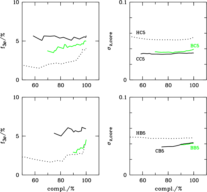
Investigating many of these characteristic lines, we find that the most obvious feature is that $\sigma_{z}$ as well as $f_{3\sigma}$ are often insensitive to a tightening of the cut criterion. This immediately tells us that the errors from the photo-$z$ codes are not proportional to the real errors on an object-by-object basis and thus of limited use. The real accuracy of the photo-$z$ is not tightly correlated with the error estimate.

The curves corresponding to Hyperz (dotted lines) show some dependence of the outlier rate, $f_{3\sigma}$, on a tightening of the cut. At some point around 80% completeness a saturation behaviour sets in and a further tightening does not decrease the outlier rates anymore. BPZ shows a similar but less pronounced behaviour. Thus, very large confidence intervals or very low ODDS values indicate that the photo-$z$ estimation failed indeed. We assume that at this point the width of the confidence interval is not dominated by the photometric errors but becomes influenced by systematic uncertainties in the photometric calibration, the template set, the filter curves or the code itself.

From the preceding paragraphs it should be clear that the choice of $A$ in Eq. 3 and Eq. 4 as a criterion for a reliable redshift estimate is somewhat arbitrary. After careful investigation of all characteristic line plots for all setups we decided to fix the cut for the rejection of uncertain objects in Hyperz at $\sigma>0.125$, in the COMBO code at $\sigma>0.15$ and in BPZ at $ODDS<0.95$. This appears to eliminate the most uncertain objects in the datasets studied here. Furthermore, the error distribution of these remaining, secure samples is close to a Gaussian for most setups if 3-sigma outliers are rejected, i.e. $\sim 68\%$ of the objects lie within their error estimate around the mean $\delta_{z}$.

There is clearly some amount of degeneracy between the quantities defined in this section. If the photo-$z$ error distribution was purely Gaussian, scatter and bias would be sufficient numbers to characterise the accuracy of one particular setup. As described above, this is not the case for real data (see also Fig. 5 & 6). Usually, there is a core which might be offset by some bias and there are very extended wings containing catastrophic outliers. This complex error distribution is not easily described by a few numbers and a specific choice must be a compromise between clarity and degeneracy.

For example, a smaller core scatter will probably produce more $3\sigma$ outliers than a larger core scatter. With no alternative at hand to condense the performance of one particular setup into a handful of numbers we can only refer to the $z_{\mathrm{phot}}$ vs. $z_{\mathrm{spec}}$ plots shown in the following which give an uncompressed view of the data.

4.2 VVDS setups

The VVDS is complete i̱n terms of observations down to $I_{\mathrm{AB}}=24$ which corresponds to $I_{\mathrm{Vega}}\approx 23.5$. Thus, we decided to asses the photo-$z$ accuracy for all objects with $17<R<23$ to achieve a reasonable level of completeness. However, we note that the fraction of VVDS objects with high-quality flags (3/4/23/24) has dropped to approximately $\sim 2/3$ compared to the whole VVDS catalogue at $R<23$. We also present the results for a fainter magnitude bin with objects in the range $23<R<24$ which are then possibly biased in terms of selection. The mean redshifts in the bright and the faint bins are $z=0.55$ and $z=0.75$, respectively.

The different setups are named with three-letter acronyms with the first letter denoting the code (“H” for Hyperz, “C” for the COMBO code, and “B” for BPZ), the second letter denoting the dataset (“B” for GaBoDS and “C” for COMBO), and the digit at the third position denoting the filter set (“5” for $UBVRI$, “4” for “BVRI”, and “17” for the full COMBO-17 filter set including medium-band-filters).

4.3 FDF setups

Since the FDF data are extremely deep and subtle trends in photometric errors make little difference to the photo-$z$ quality, we do not split the FDF sample into magnitude bins. Furthermore, given the selection choices made for the spectroscopic sample it is not complete at or representative for any particular magnitude limit. Hence, we split the FDF spectroscopic catalogue into two samples at $z=2$ to show the effects of different filter sets and especially NIR bands on the performance at low and high redshift in comparison. The FDF setups are denoted by a second letter “F” for FDF and the filter set is spelled out.

5 Results and Discussion

In the following we report the results from our blind test of photo-$z$ performance for the different setups. As a complete coverage of all possible data-code-parameter combinations would be beyond the scope of this paper we concentrate on some well-chosen setups to illustrate the effects of key parameters.

5.1 VVDS results

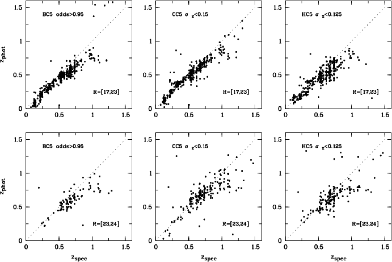
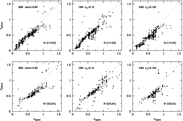
The statistics for all photo-$z$ setups that are compared to the VVDS spectroscopic catalogue are shown in Table 2 and Table 3. Selected setups are also illustrated in Fig. 5 and Fig. 6 by plots showing photo-$z$ versus spectroscopic redshift.

5.1.1 COMBO data

Clearly, the COMBO code performs best in comparison to the two other codes with the 17-filter set as well as with the 4- and 5-filter sets. While BPZ produces similar outlier rates and scatter values as the COMBO code the completeness is lower. Hyperz performs slightly worse here.

BPZ and Hyperz produce some negative biases. The cross-calibration between templates and photometry is obviously more accurate for the PEGASE templates used by the COMBO code than for the CWW, Kinney, and BC templates used by BPZ and Hyperz, respectively. Similar negative biases are found by Csabai et al. (2003) using the CWW and BC templates for photo-$z$ estimates on SDSS data.

The COMBO code shows the expected behaviour that the photo-$z$ accuracy decreases when further filters are excluded. Completeness decreases while outlier rate and scatter increase. No large biases are produced in any setup.

A very interesting fact concerning Hyperz and BPZ is that the exclusion of the $U$-band decreases the bias in the bright bin. Clearly, the photo-$z$ results with the COMBO code as well as the comparisons between the different datasets in Sect. 2.1 show that this behaviour is not caused by a badly calibrated $U$-band.

The best results in both magnitude bins are certainly achieved with the full 17-filter set of COMBO-17. Especially in the bright magnitude bin the scatter and the outlier fractions are very small compared to all 4- or 5-filter-setups. In the fainter bin, however, the difference is not as dramatic due to the lack of depth in many of the medium-bands. Hyperz also shows relatively accurate results for the 17-filter set (HC17) but not as accurate as the CC17. BC17 performs in between. In the bright bin, the proper modelling of emission lines in the PEGASE templates that can affect the flux in the medium-band filters considerably pays off for the COMBO code resulting in a very small scatter on the 0.02 level. Emission lines are not included in the BC93 templates used by Hyperz and less pronounced in the observed CWW + Kinney templates of BPZ.

5.1.2 GaBoDS

Owing to their greater depth the GaBoDS data mostly lead to better results than the shallower COMBO data, in $UBVRI$ as well as in $BVRI$. As expected, the effect is much more pronounced in the faint bin, while the depth helps less in the estimation of redshifts for high $S/N$ objects at the bright end of our catalogue. Nevertheless, also bright objects with $>20\sigma$ detections in the $R$-band can benefit from the depth in the other bands.

The negative biases in the photo-$z$ estimation with BPZ and Hyperz is also present in GaBoDS setups with the $U$-band included. At this point, it is important to mention again that the GaBoDS $U$-band filter is different from the COMBO $U$-band filter. The GaBoDS filter is wider and bluer.

For the COMBO code, the 4- and 5-filter results are nearly indistinguishable. Only in the faint bin the outlier rates increase slightly when the $U$-band is excluded. Hyperz shows the unexpected feature that most statistics become more accurate when going from five to four filters. BPZ shows a similar behaviour as the COMBO code. The statistics are nearly independent on the choice between 4- and 5-filter set. Even the bias of $\sim 0.06\,\mathrm{mag}$ in the faint bin is this time present when using just $BVRI$.

The biases for the $UBVRI$ setups may well be due to the very blue $U$-band filter used for the GaBoDS data. The filter-curve entering the photo-$z$ code is less well defined because of the strongly varying spectral throughput of the atmosphere in the near-UV and the large chip-to-chip variations in differential CCD efficiency at these wavelengths. We tried to shift the blue-cutoff of the transmission curve of the atmosphere in a reasonable range. This can slightly reduce the photo-$z$ bias but might not be reproducible. This problem is also present in the COMBO data but less severe due to the redder COMBO $U$-band.

5.1.3 Common trends

The outlier rates, $f_{3\sigma}$ produced by Hyperz are in most cases larger than the outlier rates produced by the COMBO code in corresponding setups, although for the COMBO-code-setups usually less objects are rejected. BPZ produces $f_{3\sigma}$ values which are not too different from the COMBO code. However, one should mention at this point that Hyperz gives the user a handle to get rid of some of these outliers with the drawback of decreased completeness. As described in Sect. 4.1 the outlier rate for most Hyperz setups decreases monotonically at least down to some point when objects with very large photo-$z$ error estimates are excluded.

The outlier-excluded scatter values, $\sigma_{z}$, do not show a clear trend with every code being the most accurate in at least one setup. There is clearly some amount of degeneracy between completeness, $f_{3\sigma}$, $\delta_{z}$, and $\sigma_{z}$. The plots in Fig. 5 and 6 provide a more complete view of the performance.

Remarkably, the negative biases introduced by BPZ and Hyperz as reported above are much smaller or negligible for the COMBO code. This suggests that the consistent photometric calibration of the two surveys (note that the photometry is also consistent with the MUSYC survey) is not the source of the biases. Rather the combination of these ground-based photometric datasets with particular template sets seems to be problematic. BPZ and Hyperz together with the supplied template sets are tested in their release papers (Benítez 2000; Bolzonella et al. 2000) only against real data from the Hubble Deep Field, besides simulations. BPZ now incorporates a new template set (see Sect. 3.3) that was specially calibrated for HST photometry. The COMBO code, however, was originally designed for the ground-based survey CADIS (Wolf et al. 2001), where colours were measured bias-free from seeing adaptive photometry, and included photo-$z$’s for point-source QSOs.

In general, photo-z biases can be removed by a recalibration procedure with a spectroscopic training sample. Fixing the redshift for the training set objects one can fit for zeropoint offsets in the different filters that minimise the magnitude differences between the observed object colours and best-fit template colours. We developed such recalibration methods for BPZ and Hyperz making use of the spectroscopic redshifts of the VVDS. In this way we can decrease or completely remove the biases which are still present in the blind setups. A more advanced technique incorporating also a recalibration of the template set after recalibrating the photometric zeropoints can lead to even more accurate results (see e.g. Benítez et al. 2004; Ilbert et al. 2006). We don’t refer to the recalibrated photometry in the remainder of this paper and instead focus on blind applications.

One of the biggest differences between the codes is the template set chosen and one might presume that most of the difference in performance originates from this point. However, we run Hyperz with the PEGASE templates used by the COMBO code as well as with the CWW templates plus two Kinney starburst templates originally used by BPZ in Benítez (2000). We switch off the Hyperz internal reddening because it is already included in the BPZ templates and the PEGASE age$\times$extinction grid used by the COMBO code. The results can neither compete with the best Hyperz setups incorporating the BC templates nor with the COMBO code plus PEGASE templates. Hence, the implementation of user-defined templates appears to be not straightforward and results may not be competitive with the template sets that are shipped with the code and were tested and optimised by the author.

Another interesting point is the comparison of the CC17 setup with the CB5 setup. While the total exposure time with WFI is lower for CC17, the performance of CC17 is better in all statistics described here. It is clear, that for the particular application of photo-$z$’s for bright objects, the exposure time was well spent on more filters (which is an important result for future surveys). However, the GaBoDS data of the CDFS are completely based on archive data and no specific observing programme was proposed to create these deep images. Furthermore, for deeper applications, such as Lyman-break galaxy studies, where you simply need a very deep colour index between three bands, the GaBoDS data are certainly highly superior to the COMBO data.

Table 2: Photo-$z$ errors and outlier rates for selected setups on the COMBO-CDFS data (bright sample left, faint sample right).

Sample	$R=[17,23]$				$R=[23,24]$
Mean redshift	0.55				0.75
Configuration	compl. [%]	$f_{0.15}$ [%]	$f_{3\sigma}$ [%]	$\left<\delta_{z}\right>\pm\sigma_{z}$	compl. [%]	$f_{0.15}$ [%]	$f_{3\sigma}$ [%]	$\left<\delta_{z}\right>\pm\sigma_{z}$
BC17	97.6	2.7	3.4	$-0.035\pm 0.034$	69.7	4.6	4.6	$-0.036\pm 0.038$
BC5	94.1	3.3	4.5	$-0.049\pm 0.037$	42.2	8.7	5.4	$-0.046\pm 0.053$
BC4	85.3	6.9	9.2	$-0.033\pm 0.048$	34.4	8.0	6.7	$-0.040\pm 0.046$
CC17	99.8	1.2	4.8	$-0.011\pm 0.018$	100.0	9.6	16.1	$-0.012\pm 0.027$
CC5	100.0	4.0	5.7	$-0.017\pm 0.035$	98.6	8.4	4.7	$-0.024\pm 0.065$
CC4	97.2	7.6	5.9	$-0.023\pm 0.056$	83.5	21.4	13.2	$0.001\pm 0.084$
HC17	99.8	5.2	5.7	$-0.026\pm 0.041$	99.5	16.6	16.1	$-0.032\pm 0.052$
HC5	96.9	6.8	3.7	$-0.045\pm 0.053$	83.5	15.9	6.6	$-0.045\pm 0.072$
HC4	81.3	10.5	7.0	$-0.034\pm 0.059$	73.4	16.9	10.0	$-0.049\pm 0.063$

Table 3: Same as Table 2 but for the GaBoDS-CDFS data.

Sample	$R=[17,23]$				$R=[23,24]$
Mean redshift	0.55				0.75
Configuration	compl. [%]	$f_{0.15}$ [%]	$f_{3\sigma}$ [%]	$\left<\delta_{z}\right>\pm\sigma_{z}$	compl. [%]	$f_{0.15}$ [%]	$f_{3\sigma}$ [%]	$\left<\delta_{z}\right>\pm\sigma_{z}$
BB5	97.4	2.7	3.4	$-0.037\pm 0.040$	87.7	6.7	12.4	$-0.062\pm 0.041$
BB4	88.5	3.1	10.4	$-0.010\pm 0.045$	85.0	5.3	9.6	$-0.060\pm 0.043$
CB5	99.5	3.6	4.3	$-0.024\pm 0.041$	98.6	8.8	8.8	$-0.028\pm 0.044$
CB4	99.8	4.8	3.8	$-0.019\pm 0.049$	96.8	11.4	12.3	$-0.026\pm 0.042$
HB5	95.7	9.0	3.8	$-0.065\pm 0.048$	79.1	18.4	19.0	$-0.060\pm 0.039$
HB4	74.2	4.8	5.5	$-0.034\pm 0.040$	75.5	13.3	13.9	$-0.052\pm 0.035$

Figure 5: Photo-$z$’s from the CDFS-COMBO $UBVRI$ imaging data vs. spectroscopic redshifts from the VVDS. The left column shows results for BPZ, the middle column for the COMBO code, and the right column for Hyperz. Bright objects with $17<R<23$ are shown in the top panel, faint objects with $23<R<24$ in the bottom panel.

Figure 6: Same as Fig. 5 but for the GaBoDS $UBVRI$ imaging data.

5.2 FDF results

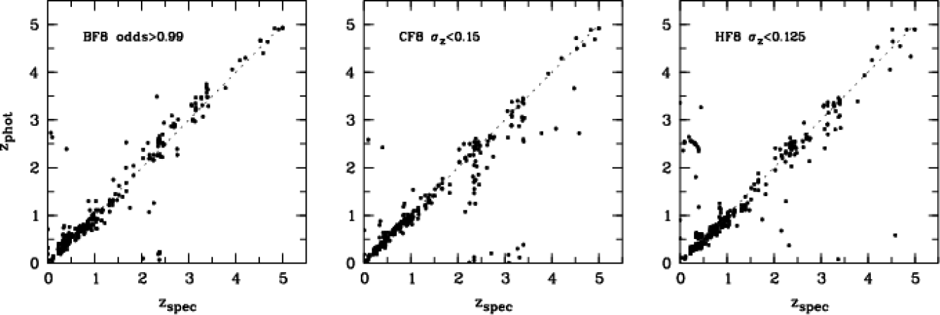
Table 4 summarises the results on the FDF and Fig 7 shows photometric vs. spectroscopic redshift for selected setups. In the lower redshift bin again the COMBO code combined with imaging data in 8 filters delivers the smallest outlier rate, bias, and scatter when compared to BPZ and Hyperz in 8 filters. At least in this redshift interval the results are nearly as good as the results produced by Gabasch et al. (2004) with a template set specifically calibrated for the FDF.

In the high redshift domain, however, the COMBO code does not perform well with an outlier rate and scatter twice as large as the ones produced by Hyperz and with a considerable bias. BPZ performs not too different from Hyperz. Apparently, the COMBO code in combination with the PEGASE templates has problems when the Lyman break enters the filter set: many objects appear at too low redshifts, hence the large negative bias (see also Fig 7). The inferior performance in the high redshift domain can then be attributed to colour-redshift-degeneracies described in detail in Benítez (2000). Basically, a larger number of templates can lead to better low-$z$ performance with the tradeoff of poorer high-$z$ performance due to increasing degeneracies. Designed for medium-deep surveys the COMBO code was naturally not optimised to work at high redshifts in contrast to BPZ and Hyperz. There, the application of a Bayesian prior on the apparent magnitude combined with a sparse template set (BPZ) or a top-hat prior on the absolute magnitude (Hyperz) delivers significantly better results.

The dependence of photo-$z$ performance on the filter set is also shown in Table 4. In the lower redshift interval the outlier rate nearly doubles as soon as the NIR filters $J$ and $K_{s}$ are dropped. The scatter, however, remains nearly constant. Without near-infrared data a larger negative bias is introduced which was already present in all VVDS-Hyperz setups (see Table 2 and 3). The exclusion of the peculiar $U$-band reduces this bias again with the drawback of increased scatter. In the higher redshift domain results get much worse when near-infrared data are dropped.

Figure 7: Photometric vs. spectroscopic redshifts for the FDF full 8-filter set imaging data. The left diagram shows results for BPZ, the middle diagram for the COMBO code, and the right diagram for Hyperz.

Table 4: Same as Tables 2 and 3 but for the FDF data (low-$z$ sample left, high-$z$ sample right).

Sample	$z=[0,2]$				$z=[2,5]$
Mean redshift	0.65				2.94
Configuration	compl. [%]	$f_{0.15}$ [%]	$f_{3\sigma}$ [%]	$\left<\delta_{z}\right>\pm\sigma_{z}$	compl. [%]	$f_{0.15}$ [%]	$f_{3\sigma}$ [%]	$\left<\delta_{z}\right>\pm\sigma_{z}$
BF_UBgRIZJKs	98.1	5.4	5.4	$0.005\pm 0.053$	93.3	12.0	13.3	$0.026\pm 0.046$
CF_UBgRIZJKs	99.6	3.4	4.9	$0.001\pm 0.034$	100.0	29.2	13.5	$-0.046\pm 0.093$
HF_UBgRIZJKs	99.6	10.2	9.8	$-0.019\pm 0.051$	100.0	8.0	5.7	$-0.004\pm 0.056$
BF_UBGRIJKs	98.5	8.4	9.2	$0.011\pm 0.058$	89.9	18.8	18.8	$0.024\pm 0.050$
BF_UBGRIZ	97.7	7.7	9.6	$-0.010\pm 0.041$	91.0	17.3	19.8	$0.032\pm 0.047$
BF_UBGRI	98.1	8.4	9.2	$0.000\pm 0.042$	74.2	27.3	27.3	$0.025\pm 0.057$
BF_BGRI	90.2	12.5	8.3	$0.020\pm 0.060$	53.9	27.1	27.1	$0.017\pm 0.051$
CF_UBGRIJKs	99.6	4.5	4.5	$0.006\pm 0.044$	95.5	30.6	14.1	$-0.058\pm 0.102$
CF_UBGRIZ	99.6	6.0	7.9	$-0.006\pm 0.039$	98.9	54.5	47.7	$-0.061\pm 0.077$
CF_UBGRI	96.6	5.8	7.0	$-0.001\pm 0.043$	94.4	57.1	38.1	$-0.100\pm 0.082$
CF_BGRI	92.5	16.3	13.0	$0.006\pm 0.066$	93.3	62.7	50.6	$-0.095\pm 0.099$
HF_UBGRIJKs	99.6	10.2	10.6	$-0.022\pm 0.049$	100.0	9.1	8.0	$-0.012\pm 0.053$
HF_UBGRIZ	100.0	12.8	11.7	$-0.020\pm 0.048$	100.0	12.5	12.5	$0.009\pm 0.052$
HF_UBGRI	99.2	14.4	17.8	$-0.028\pm 0.040$	97.7	20.9	14.0	$-0.012\pm 0.072$
HF_BGRI	99.6	19.6	22.6	$-0.021\pm 0.038$	96.6	24.7	16.5	$-0.010\pm 0.086$

6 Photo-$z$ vs. photo-$z$ comparisons

With photo-$z$ estimates for the complete imaging catalogues at hand we cannot only compare photo-$z$’s to spectroscopic redshifts but we can also compare the different photo-$z$’s to each other. In this way we are able to detect possible selection effects that might still be present in the secure spectroscopic subsamples used in the preceding sections.

We define similar quantities as in Sect. 4 but now with the spectroscopic redshift replaced by another photo-$z$. Since none of the two photo-$z$’s is superior to the other in general, the interpretation of the statistics changes then. For example, a catastrophic disagreement between two photo-$z$ estimates just means that at least one of the two is wrong, but it can also be true that both are wrong.

Due to these complications we can learn most from comparing the photo-$z$ vs. photo-$z$ benchmarks for different subsamples. In the following, we will look at the complete CC5 catalogue and compare these redshift estimates with CB5. Moreover we compare CB5 to HC5. Thus, we study how the performance is either affected by additional depth or by using a different code. Two samples are considered, the whole catalogue with $17<R<23$ and the subsample with secure spectroscopic redshifts used before. Any significant statistical difference in these photo-$z$ vs. photo-$z$ comparisons can be interpreted then to be due to selection effects in the spectroscopic subsample.

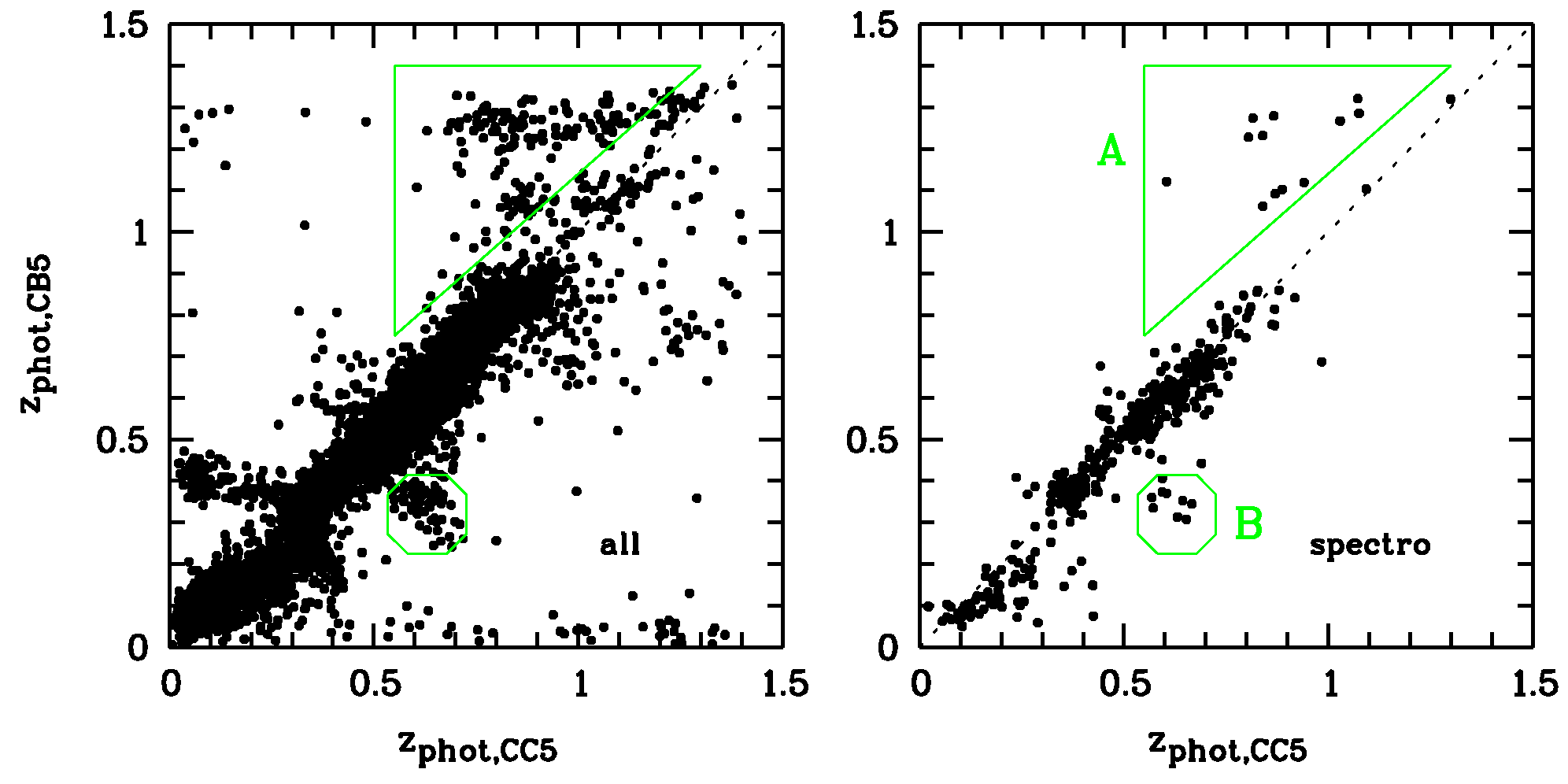
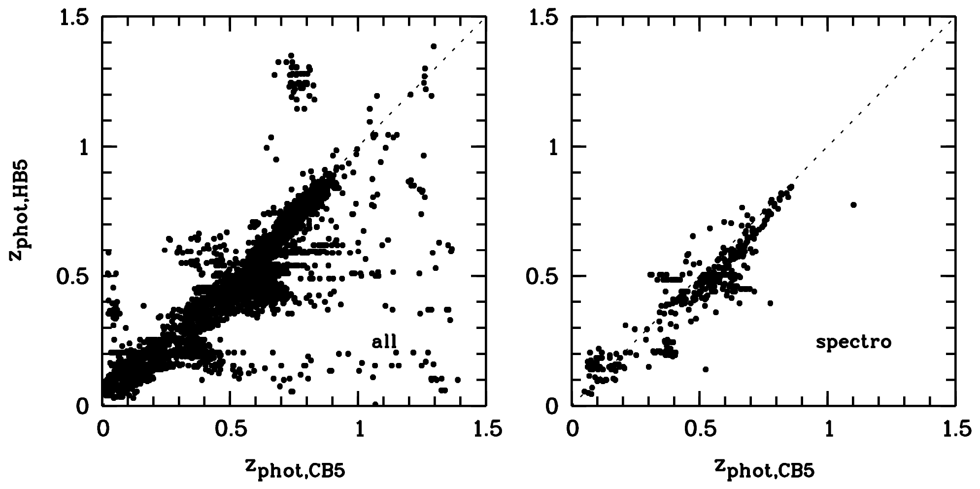
Figures 8 & 9 show the results for a comparison of photo-$z$’s from data of different depths and from different codes, respectively. The statistics are summarised in Table 5. We require an object to meet the criteria defined in Sect. 4.1 for both photo-$z$ setups entering the comparison.

There are some distinctive features visible in Fig. 8. The ones labelled “A” and “B” can be found in in both panels and just the overall number density in the left panel is larger by a factor of 14. Two other features, one clump at $z_{\mathrm{p}hot,CC5}=0.0-0.3$ and $z_{\mathrm{p}hot,CB5}\sim 0.4$ and a couple of outlier objects at $z_{\mathrm{p}hot,CC5}=0.5-1.5$ and $z_{\mathrm{p}hot,CB5}=0.0-0.1$, are however, only found in the photometric sample and not in the spectroscopic one.

Even more striking is the difference in the overall distributions of objects when the two codes are compared in Fig. 9.

This is also reflected in the numbers. The outlier rates, $f_{0.15}$, for the full sample are larger by a factor of $\sim 2$ when comparing data depth (CC5 vs. CB5) and $\sim 4$ when comparing codes on identical data (CB5 vs. HB5). Completeness and scatter are essentially the same for both subsamples while the bias slightly increases from “CB5 vs. HB5, all” to “CB5 vs. HB5, spectro”.

This means that the properties of the core of the $\Delta z$ distribution are quite similar for both samples but that the wings are more pronounced when all objects are considered. Apparently, the secure spectroscopic subsample represents an intrinsically different galaxy population than the full, purely magnitude-limited sample. The rejection of objects with bad spectroscopic flags introduces a bias in the spectroscopic sample so that it is no longer purely magnitude-limited and artificially reduces the apparent outlier rates.

Figure 8: Photo-$z$ vs. photo-$z$ for the COMBO code run on the $UBVRI$ imaging data from COMBO (CC5) and from GaBoDS (CB5). The left diagram shows results for the full sample and the right diagram for the secure spectroscopic subsample. In this plot the objects rejected by the criteria from Sect. 4.1 are not shown. The object density in the left plot is 14 times higher than in the right one.

Figure 9: Same as Fig. 8 but with photo-$z$ vs. photo-$z$ for the COMBO code (CB5) and Hyperz (HB5) run on the GaBoDS $UBVRI$ imaging data.

Table 5: Statistics for the comparison between the different photo-$z$’s.

Sample	$R=[17,23]$
Configuration	compl. [%]	$f_{0.15}$ [%]	$f_{3\sigma}$ [%]	$\left<\delta_{z}\right>\pm\sigma_{z}$
CC5 vs. CB5, all	99.4	6.3	9.7	$-0.007\pm 0.035$
CC5 vs. CB5, spectro	100.0	3.2	9.8	$-0.006\pm 0.030$
CB5 vs. HB5, all	92.6	9.0	8.7	$-0.033\pm 0.053$
CB5 vs. HB5, spectro	95.7	2.5	2.8	$-0.057\pm 0.047$

7 Summary and Conclusions

We have shown that photo-$z$’s estimated with today’s tools can produce a reasonable accuracy. The performance of a particular photo-$z$ code, however, cannot easily be characterised by a mere two numbers such as scatter and global outlier rate. The benchmarks are rather sensitive functions of filter set, depth, redshift range and code settings. Moreover, there is at least a factor of two possible difference in performance between different codes which is again not stable for all setups but can vary considerably from one setup to another. There are, for example, redshift ranges where one code clearly beats another one in terms of accuracy only to loose at other redshifts. We give estimates of the performance for a number of codes in some practically relevant cases.

The estimation of photo-$z$’s from different ground-based datasets is not straightforward and results should not be expected to be identical to simulated photo-$z$ estimates. Rather, photo-$z$ simulations often seem to circumvent critical steps in ground-based photo-$z$ estimation. Most importantly, the match between observed colours and some template sets commonly used may be suboptimal.

In the preceding sections we have identified several aspects which are relevant to future optimisations of photo-$z$ codes. The photo-$z$ error estimation is one of the most unsatisfying aspects to date with error values often only very weakly correlated with real uncertainties. This is likely due to the insufficient inclusion of systematics since very low S/N objects, for which the errors should be dominated by photon shot-noise, show a tighter correlation. Chip-to-chip sensitivity variations, especially in the UV, could either be taken into account more accurately within the photo-$z$ codes or could be tackled by improved instrument design, survey strategy, and data reduction. The optimisation of template sets can be expected to be successfully done with ever larger spectroscopic catalogues becoming available.

In general, biases can be removed by a recalibration which requires an extensive spectroscopic training set. Another proven successful route to better photo-$z$’s is improving the spectral resolution of the data, instead of their depth, as demonstrated by the COMBO-17 survey. This approach is also taken by the new ALHAMBRA survey (Moles et al. 2005, Benítez et al., 2007, A&A, submitted) and COSMOS-21.

A general problem for all studies comparing photo-$z$’s to spectroscopic redshifts is our finding that secure spectroscopic samples can be biased. While surveys like VVDS are $>90\%$ complete in obtaining spectra for galaxy samples the redshifts that are claimed to be $>90\%$ secure only amount to $\sim 50\%$. This subsample obviously consists of galaxies for which the photo-$z$ estimation works better than for the whole sample. In the future, it is desirable to put effort into spectroscopic surveys with secure redshift measurements for virtually every galaxy down to the same flux limit that is used for the analysis of photo-$z$ samples.

Several questions that are raised in this work will be tackled by the PHAT initiative mentioned above. PHAT aims to understand the issues presented here in a systematical and quantitative way in order to give guidance for better photo-$z$’s in the future.