A Search for sub-km KBOs with the Method of Serendipitous Stellar Occultations

Abstract

The results of a search for sub-km Kuiper Belt Objects (KBOs) with the method of serendipitous stellar occultations are reported. Photometric time series were obtained on the 1.8m telescope at the Dominion Astrophysical Observatory (DAO) in Victoria, British Columbia, and were analyzed for the presence of occultation events. Observations were performed at 40 Hz and included a total of 5.0 star-hours for target stars in the ecliptic open cluster M35 ($\beta=0.9\arcdeg$), and 2.1 star-hours for control stars in the off-ecliptic open cluster M34 ($\beta=25.7\arcdeg$). To evaluate the recovery fraction of the analysis method, and thereby determine the limiting detectable size, artificial occultation events were added to simulated time series (1/f scintillation-like power-spectra), and to the real data. No viable candidate occultation events were detected. This limits the cumulative surface density of KBOs to $3.5\times 10^{10}$ deg^-2 (95% confidence) for KBOs brighter than m_R=35.3 (larger than $\sim$860m in diameter, assuming a geometric albedo of 0.04 and a distance of 40 AU). An evaluation of TNO occultations reported in the literature suggests that they are unlikely to be genuine, and an overall 95%-confidence upper limit on the surface density of $2.8\times 10^{9}$ deg^-2 is obtained for KBOs brighter than m_R=35 (larger than $\sim$1 km in diameter, assuming a geometric albedo of 0.04 and a distance of 40 AU) when all existing surveys are combined.

1. Introduction

The physical and orbital properties of the Kuiper Belt Objects (KBOs) are believed to provide valuable information about the formation of the solar system. To date, directly observed KBOs include objects with diameters ranging from $\sim$25km (eg. 1999 DA₈, Gladman et al. 2001; and 2003 BH₉₁, Bernstein et al. 2004) to 2400km (eg. Eris, Brown et al. 2006). KBOs with diameters below a few tens of kilometers are beyond the detection of current ground and space-based telescopes.

The KBO size distribution is the outcome of accretion and collisional evolution in the outer solar system (Stern 1996; Davis & Farinella 1997; Stern & Colwell 1997; Kenyon & Luu 1999b; Kenyon & Bromley 2004; Pan & Sari 2005). The cumulative luminosity function (CLF) of the KBOs provides an indirect means of determining their size distribution, and is observed to have the form: $\sum N(<m_{R};m_{R}<25)=10^{\alpha(m_{R}-R_{0})}$. The KBO size distribution is then a power-law of the form: $\mathrm{d}N\propto r^{-q}\mathrm{d}r$, with slope $-q$, where $q$ is related to $\alpha$ via: $q=5\alpha+1$ (Gladman et al. 2001, G01). Current observations indicate $\alpha\approx 0.68$ (Fraser et al. 2007), or equivalently, $q=4.6$. HST observations by Bernstein et al. (2004) suggest a lower CLF slope for $m_{R}>25$.

Current theoretical models of the accretion and fragmentation processes in the early solar system suggest that $q$ remains constant only for larger objects, and that the slope of the size distribution changes at the ‘break radius’, $r_{b}<$100 km (Kenyon & Luu 1999a, b; Kenyon & Bromley 2004; Pan & Sari 2005). Objects smaller than the break radius would be in collisional equilibrium and their size distribution would have the so-called Dohnanyi equilibrium slope of $q\approx 3.5$ (Dohnanyi 1969). Object densities and bulk-moduli can influence the slope for the small objects, and the position of the break-radius (Kenyon & Bromley 2004).

The deepest direct observations to date (Bernstein et al. 2004) were performed with HST and reached a limiting magnitude of R=28.5 (corresponding to an object diameter of $\sim$20km for an albedo of 0.04 at 40AU). The number of observed objects was $\sim$25$\times$ lower than the extrapolation of the current CLF slope. This absence of faint objects indicates a decrease in the density of the Kuiper Belt beyond 50 AU; and a dearth of sub-100km KBOs, in general. Direct observation is not a feasible option for pursuing the much fainter km-sized KBOs.

Some indirect methods of inferring the slope in the range of the km-sized objects have been explored. Stern & McKinnon (2000) used Voyager 2 images of Neptune’s moon Triton to analyze cratering and infer a slope of $q\approx 3$ for the size distribution of the km-sized impactors. Kenyon & Windhorst (2001) have placed upper limits on small object densities by examining the optical and FIR sky surface brightnesses of the ecliptic. They found that a straight extrapolation of the CLF to R$\approx$40-50 mag would yield an ecliptic surface brightness higher than that observed.

One promising method of indirect detection for the smaller KBOs is that of serendipitous stellar occultations (Bailey 1976; Dyson 1992; Brown & Webster 1997; Roques & Moncuquet 2000; Cooray 2003; Cooray & Farmer 2003; Gaudi 2004; Nihei et al. 2007). A km-sized KBO passing through the line of sight to a star will partially obscure the light from that star to reveal the presence of the otherwise invisible object. Such an occultation cannot be predicted and the practice relies upon serendipity.

A 1 km diameter KBO at 40AU subtends and angle of only 34 $\mu$as, and the lightcurve resulting from an occultation by such an object is expected to exhibit a series of increases and decreases due to diffraction (Roques et al. 1987) (henceforth R87). At opposition, the orbital velocities of the Earth (30 $\mathrm{km\ s}^{-1}$ ) and a typical KBO at 40 AU ($\sim$4 $\mathrm{km\ s}^{-1}$ ) produce a retrograde relative velocity of $v\approx$26 $\mathrm{km\ s}^{-1}$ for the occulter, and the characteristic diffraction shadow cast by a 1 km KBO will pass over a terrestrial observer in a fraction of a second. Observations must be performed at $\geq$40 Hz to sample the flux oscillation in an observed lightcurve.

We have performed a KBO occultation search with the 1.8m Plaskett Telescope at the Dominion Astrophysical Observatory (DAO) using a 40Hz camera. Models of occultation lightcurves are presented in Section 2. Observation details are given in Section 3, with data reduction and analysis methods described in Sections 4, and 5, respectively. Our results are presented in Section 6, and reported KBO occultation detections are evaluated in Section 7. A surface density upper limit is presented in Section 8, with a discussion and summary provided in Sections 9 and 10, respectively.

2. Modeling Occultations

The object diameter at which diffraction effects begin to dominate a KBO occultation lightcurve is known as the Fresnel scale, $\rho=\sqrt{\lambda z/2}$, where $\lambda$ is the wavelength and $z$ is the distance between the observer and the occulting body. For a KBO occultation ($z$=40AU) observed in visible light (550nm), the Fresnel scale is 1285m. Fresnel-Kirchhoff diffraction theory should be used to model occultation lightcurves for objects with sizes of order 1 Fresnel scale unit (Fsu). Following R87, we have modeled occulters as circular disks, with the masking disk assembled by placing progressively smaller rectangular masks at the periphery of the structure. Five ‘orders’ of such rectangles were used for our models. An analytic circularly-symmetric solution to the Fresnel-Kirchhoff equation exists (R87), but we chose to develop our KBO disks from assemblies of rectangles to build in flexibility of object shape for future work.

2.1. Passbands and Source Dimensions

Intensities were numerically integrated over a range of wavelengths to model a broadband observation of an occultation. This was accomplished by averaging evenly-weighted diffraction patterns at wavelengths distributed uniformly across the passband. Lightcurves for 550nm monochromatic light and 400-700nm broadband light are compared in Figure 1. The extended ‘ringing’ present in the monochromatic pattern is attenuated by interference in the broadband pattern; only the first peak away from the pattern center is well preserved.

Figure 1.— Diffraction profiles for monochromatic light (550nm) and broadband visible light (400-700nm). The occulting object was 250m in radius at a distance of 40AU.

It was unnecessary to weight the intensities to match the spectral energy distribution (SED) of the target star, the spectral throughput of the telescope, and the spectral sensitivity of the CCD. Even-weighting offered greater precision than needed for work with photometric time series having $\gtrsim 1$% RMS variability.

The target stars were modeled by averaging evenly-spaced point sources over the projected stellar disks. A point source density of 100 Fsu^-2 was used ($\sim$100 points for the stellar disks of the M35 targets projected at 40 AU). This density was more than sufficient to provide an accurate model of the shadow, consistent with models found in Roques & Moncuquet (2000).

2.2. Conversion of the Shadow Profile to a Time Series Profile

Intensities for the diffraction-dominated occultation shadows were computed as a function of position with respect to the center of the projected shadow. The relative velocity was used to convert positional coordinates to time coordinates to determine the corresponding lightcurve that would be recorded by an observer passing through such a shadow.

An object observed at a given ecliptic latitude must have an orbital inclination equal to, or greater than, that latitude. As the fraction of TNOs is observed to decrease with increasing orbital inclination (Jewitt et al. 1996; Brown 2001); an observed object is most probably very near its highest latitude, where its velocity vector lies nearly parallel to the ecliptic plane. As only the ecliptic latitude of observation is known, the orbital inclination was taken to be equal to the ecliptic latitude. This is the most probable configuration, and it is illustrated in Figure 2.

Figure 2.— The orbital geometry used to derive the relative velocity of a body orbiting on an inclined orbit. Vectors labeled ’$\mathbf{r}$’ and ’$\mathbf{v}$’ denote heliocentric distance and velocity, respectively. The vector ’$\mathbf{d}$’ is the distance from the Earth to the occulting KBO. The subscript ’k’ denotes parameters referring to a KBO, and ’e’ denotes those referring to the Earth. The subscript ’p’ is used to indicate quantities projected onto the ecliptic. The Earth and KBO are indicated with $\oplus$, and $\bullet$ symbols, respectively. The angle $\varepsilon$ is the solar elongation projected onto the ecliptic plane. The angles $\alpha$ and $\beta$ are measured in the ecliptic plane; $\alpha$ measures the angle between the position vector of the Earth, $\mathbf{r}_{e}$, and the line-of-sight to the target star projected onto the ecliptic plane, $\mathbf{r}_{*p}$ ($\mathbf{r}_{*p}$ is parallel to $\mathbf{d}_{p}$).

The relevant velocity is the component of the relative velocity projected onto the plane perpendicular to the line-of-sight. Letting $\theta$ represent the angle between the line-of-sight, $\vec{d}$, and the relative velocity vector, $\vec{v_{rel}}$, that component is $v_{rel-perp}=|\vec{v_{rel}}|\sin(\theta)$. Calculation of $\theta$ can be performed with the dot product $\vec{d}\cdot\vec{v_{rel}}$:

$$\theta=\arccos\left(\frac{\mathbf{d}\cdot\mathbf{v}_{rel}}{|\mathbf{d}||\mathbf{v}_{rel}|}\right).$$ (1)

The vectors $\mathbf{d}$ and $\mathbf{v}_{rel}$ were expressed in Cartesian coordinates in terms of the quantities displayed in Figure 2. The quantities: $r_{kp}$ (heliocentric distance to the KBO projected onto the ecliptic place); angles $\beta$, and $\alpha$; and $d_{p}$ (observer-to-KBO distance projected onto the ecliptic) were determined.

$$|\mathbf{r}_{kp}|= \ |\mathbf{r}_{k}|\ \cos(i),$$ (2)

$$\beta= \ \sin^{-1}\left(\frac{\sin(\varepsilon)}{|\mathbf{r}_{kp}|}\right),$$ (3)

$$\alpha= \ \pi-\varepsilon,$$ (4)

$$|\mathbf{d}_{p}|= \ \sqrt{|\mathbf{r}_{kp}|^{2}+|\mathbf{r}_{e}|^{2}-2\ |\mathbf{r}_{kp}|\ |\mathbf{r}_{e}|\ \cos(\alpha-\beta)}.$$ (5)

The position coordinates are:

$$(x_{e},\ y_{e},\ z_{e})= \ \ (|\mathbf{r}_{e}|,\ 0,\ 0),\quad\mathrm{and}$$ (6)

$$(x_{k},\ y_{k},\ z_{k})= \left(\begin{array}[]{c}|\mathbf{r}_{kp}|\cos(\alpha-\beta)\\ |\mathbf{r}_{kp}|\sin(\alpha-\beta)\\ |\mathbf{r}_{k}|\sin(i)\end{array}\right).$$ (10)

The velocity components are:

$$(v_{xe},\ v_{ye},\ v_{ze})= (0,\ |\mathbf{v}_{e}|,\ 0),\quad\mathrm{and}$$ (11)

$$(v_{xk},\ v_{yk},\ v_{zk})= \left(\begin{array}[]{c}-|\mathbf{v}_{k}|\sin(\alpha-\beta)\\ |\mathbf{v}_{k}|\cos(\alpha-\beta)\\ 0\end{array}\right).$$ (15)

The vectors $\mathbf{d}$, and $\mathbf{v}_{rel}$ are then:

$$\mathbf{d}= (x_{k}-x_{e},\ y_{k}-y_{e},\ z_{k}-z_{e}),\quad\mathrm{and}$$ (16)

$$\mathbf{v}_{rel}= (v_{xk}-v_{xe},\ v_{yk}-v_{ye},\ v_{zk}-v_{ze})$$ (17)

Vectors $\mathbf{d}$ and $\mathbf{v}_{rel}$ were substituted into Equation 1 to compute $\theta$; and, in turn, the perpendicular component of the relative velocity $v_{rel-perp}=|\mathbf{v}_{rel}|\sin(\theta)$.

If $\mathbf{r}_{kp}$ is less than $\mathbf{r}_{e}$, the algorithm will fail for certain elongations as they no longer exist. For example, an object on an orbit with $\mathbf{r}_{kp}<\mathbf{r}_{e}$ cannot be observed at opposition; its projected position is in the same hemisphere as the sun.

3. Observations

The open clusters: M35 ($\beta=0.9\arcdeg$ N), and M34 ($\beta=25.7\arcdeg$ N) were chosen as our primary target field, and our off-ecliptic control field, respectively. Two adjacent stars were monitored in each field. The properties of the targets are listed in Table 1. Values of m_V, B-V, and the spectral (MK) types for the M34 stars were taken from Kharchenko et al. (2004). Those for M35 were taken from Sung & Bessell (1999), but the spectral types were not available and had to be inferred by comparison of M_V and B-V values to those for other upper main sequence stars of known spectral type (reported in Kharchenko et al. 2004) in the cluster. Values for the stellar radii, R^∗, were estimated based on their spectral types (Cox 2000). The distance moduli (Sarajedini et al. 2004) were used to compute the distances with $(m-M)_{V}=5\ \mathrm{log}(d)-5$. Values of $R^{*}_{\mathrm{40AU}}$ denote the stellar radii projected at 40 AU. Both clusters are sufficiently distant that the selected stars have projected diameters less than the Fresnel scale for visible light at 40AU ($\sim$1300m).

Table 1Properties of the stars in the target field (M35), and control field (M34).

	M34 Targets
Position	East (left)	West (right)
ID	TYC-2853-22-1	TYC-2853-679-1
RAJ2000	02:41:58.31	02:41:56.78
DecJ2000	+42:47:29.7	+42:47:22.4
$\beta$	25.7$\arcdeg$ N	25.7$\arcdeg$ N
mV	8.360	8.444
B-V	0.002	-0.005
MK	B9V	B9Vp Mn
R⋆	3.0 $\mathrm{R}_{\odot}$	3.0 $\mathrm{R}_{\odot}$
R${}^{\star}_{40\mathrm{AU}}$	640m	640m
(m-M)V	8.98$\pm$0.06	8.98$\pm$0.06
Dist.	625$\pm$17 pc	625$\pm$17 pc
	M35 Targets
Position	East (left)	West (right)
ID	TYC-1877-704-2	TYC-1877-266-1
RAJ2000	06:09:20.75	06:09:18.50
DecJ2000	+24:22:08:6	+24:22:05.4
$\beta$	0.9$\arcdeg$ N	0.9$\arcdeg$ N
mV	10.656	9.764
B-V	0.178	0.167
MK	B9V	B9V
R⋆	3.0 $\mathrm{R}_{\odot}$	3.0 $\mathrm{R}_{\odot}$
R${}^{\star}_{40\mathrm{AU}}$	360m	360m
(m-M)V	10.21$\pm$0.12	10.21$\pm$0.12
Dist.	1101$\pm$60 pc	1101$\pm$60 pc

Observations were conducted in 2-3″seeing conditions with the 1.8m Plaskett Telescope at the Dominion Astrophysical Observatory (DAO) on the UT nights of 2004 January 2, and 2004 January 3. These dates were chosen to place the primary target near an elongation of $\varepsilon=180\arcdeg$, where occultation probability is highest (Roques & Moncuquet 2000). On those dates, the solar elongations of M35 and M34 were $\varepsilon=169\arcdeg$, and $\varepsilon=128\arcdeg$, respectively.

A Texas Instruments TC253-SPD CCD was operated with a San Diego State University 2 (SDSU2) controller, and data were binned 8$\times$8, and sub-rastered down to a smaller region of the chip to enable the CCD to be read-out at 40Hz. The binned pixel scale was 2.67″ pixel^-1. Images taken early in the observing run were 30$\times$24 pixels, and images taken later were 25$\times$16 (8$\times$8 binned, unprocessed sizes). One hundred images were taken in repeated sequences, and were stored in 3D-FITS format. Each was followed by a $\sim$0.5s overhead as the controller initiated the next 100-frame sequence. In total, 357,000 images were obtained for M34, and 794,000 were obtained for M35.

4. Data Reduction

A bias frame was constructed by median-combining 3600 25ms dark exposures. The count level was $\sim$3000 ADU with an estimated sky contribution of $\sim$2 ADU. One thousand 100ms sky-flat calibration images were median-combined to produced a flat which showed no structure and had pixel-to-pixel variability of less than 1%. The true variability across the field was, therefore, assumed to be negligible, and no flat-field correction was applied. Examples of raw and pre-processed images are shown for the M35 field in Figure 3.

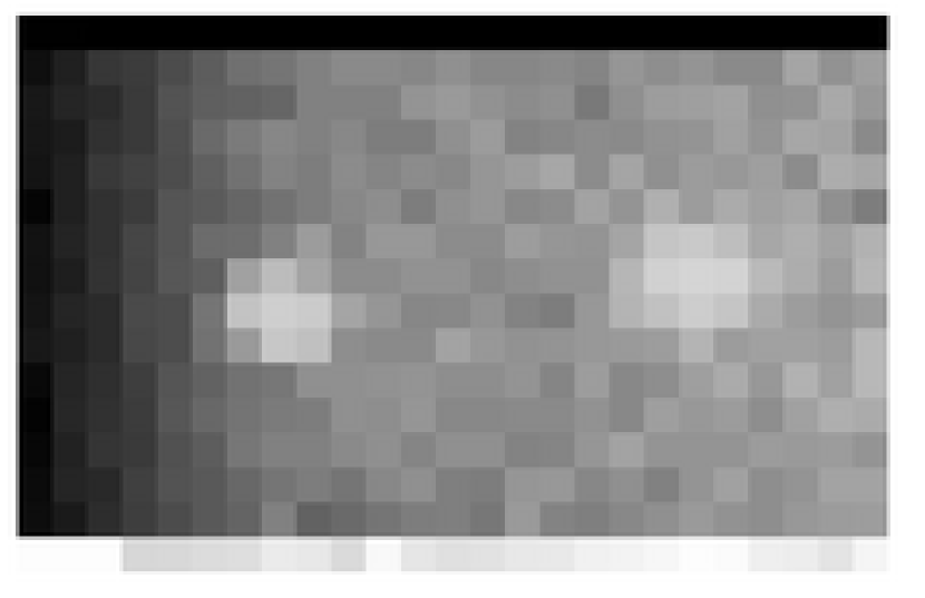
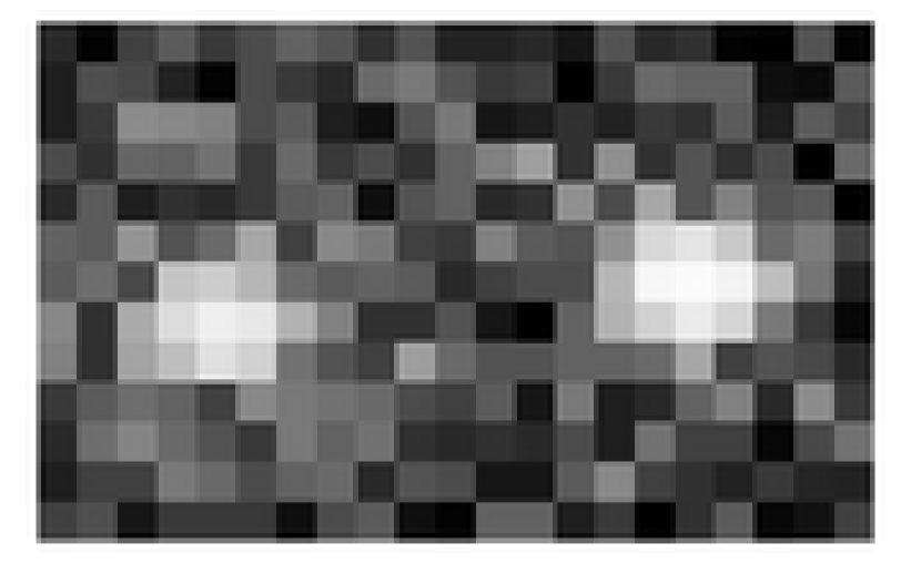
Figure 3.— Unprocessed (left) and a pre-processed (right) M35 frames. The frames are 25$\times$16 pixels, and 21$\times$12 pixels, respectively. With 8$\times$8 binning, the processed image is 56$\arcsec\times$32$\arcsec$.

As the high-speed camera was installed in place of the guider, guiding was unavailable during the observations. Without guiding, the Plaskett telescope’s tracking motor introduced an oscillation in right ascension with an amplitude of $A\approx 8$ arcsec, and a period of $T\approx$4 minutes. This corresponds to a maximum drift speed across the chip of $2\pi A/T\approx$0.2 arcsec s^-1, or 0.08 pixels s^-1. The target star’s motion between pixels was too small to induce a calibration error on the sub-second time scale of a KBO occultation.

Photometry was performed with SExtractor v2.3 (Bertin & Arnouts 1996). The stars in the field were not crowded, and aperture photometry was performed with 5 pixel (13.3 arcsec) apertures (diameter). Other SExtractor parameters were set at their default values. Flux values for the targets in the 100-frame sequences were concatenated into longer sequences of $\sim$50,000 – 100,000 frames. The 0.5s gaps occurring between the sequences were masked and ignored. The gaps are cosmetically unappealing, but only diminish the usefulness of the data in proportion to the duty cycle reduction they represent ($\sim 17\%$).

Each time series was normalized to have a constant mean flux. A sufficiently large number of simultaneously observed targets would make it possible to normalize by dividing by the summed flux of the other targets. With two targets of comparable brightness, this method would have increased the noise level in a time series by $\sim$40% ($\sqrt{2}$). Each time series was therefore normalized by dividing by a Gaussian-smoothed version of itself. To construct smoothed time series, each point was replaced by the Gaussian-weighted average of the flux measurements preceding it and following it, such that for flux $f$, the smoothed flux at the $j^{th}$ time coordinate was:

$$f_{j}=\frac{\sum_{i}w_{ij}f_{i}}{\sum_{i}w_{ij}},$$ (18)

where $w_{ij}$ is a Gaussian having a ‘width’ of $2\sigma=1$s, truncated at $\pm 3\sigma$.

$$w_{ij}=\frac{1}{\sqrt{2\pi}\sigma}e^{\frac{-(x_{i}-x_{j})^{2}}{2\sigma^{2}}}.$$ (19)

Simulated occultation lightcurves with no noise were normalized in the same way to evaluate the effects of smoothing on the events being sought. The amplitudes of these events were found to change by $<$0.5%, indicating that the normalization does not significantly attenuate or suppress an occultation signal.

Figure 4 shows a segment of a time series for the eastern-most star in the M35 field. The smoothed time series is superimposed, and the normalized time series is shown in a separate panel.

Figure 4.— A 10s sample of the time series for the eastern star in the M35 field. Both the raw flux counts (top) and the normalized data (bottom) are shown. The smoothed normalization curve is shown superimposed over the raw flux. Gaps mark the dead time of the camera.

Imaging continued through periods of reduced transparency, or partial cloud. When a star’s measured flux dropped by more than $\sim$30% in a given time segment, the noise levels in that time segment increased accordingly by $\sim$15% ($\sqrt{N}$ photon statistics), and the segment was masked.

The RMS noise values of the observed flux were computed for each target. The variates included all data for a given source; they represent the overall observation quality. A 3$\sigma$-clipped standard deviation was used to avoid the influence of outliers. The eastern and western stars in the M35 field had noise levels of $\sim$4.3% and $\sim$3.4%, respectively. Both stars in the M34 field had noise levels of $\sim$1.6%.

5. The Detection Algorithm

An object with a diameter $\gtrsim$1 Fsu (1285m for visible light at 40 AU) will produce a $>$40% flux decrease during occultation. No such events were found and a cross-correlation detection algorithm was used to search for events caused by sub-Fresnel-scale objects near the noise limit.

Template diffraction patterns were cross-correlated with each time series to detect candidate occultation events. For a discretely-sampled time series, $t_{i}$, and a template ‘kernel’, $k_{i}$, the cross-correlation is (see Bracewell 1986):

$$(t\star k)_{j}\equiv\sum_{i}t_{i}\ k_{i+j}.$$ (20)

A positive peak in $(t\star k)_{j}$ indicates that $t$ is similar to $k$ when $k$ is offset to position $j$. The detection threshold was set to $>+6\sigma_{t\star k}$ (random probability $\lesssim 10^{-9}$).

Masked data (gaps and high-noise regions) were ignored by the algorithm, and the total on-source observing time is the number of non-masked points times the individual exposure time.

To construct detection kernels for cross-correlation, theoretical occultation lightcurves were integrated and normalized in 0.025s segments to reproduce the effect of a camera taking exposures of that duration (our exposure time). Typically, 8-12 points were sufficient to model a kernel.

At 40 Hz sampling, the diffraction features of a KBO occultation lightcurve are slightly under-sampled. A small shift in the sample start time produces subtle changes in the structure of the resulting kernel, and the cross-correlation could not be performed with kernels for all possible time-shifts. To construct detection-kernels, the integration start-time was synchronized with the event such that the kernel produced would be symmetric, and this single kernel was used as the the detection-kernel. Simulated occultation-kernels which were planted in a time series for testing purposes, were integrated with a random start-time. Simulated occultation events were ‘planted’ in time series to evaluate the performance and recovery limits of the cross-correlation algorithm. For each planted event, a position in the time series was chosen randomly, and the relevant points in the time series were multiplied by the corresponding intensities from the kernel.

5.1. Performance of the Detection Algorithm

Artificial time series were used to assess the performance of the detection algorithm as they were certain to contain no occultations. Analysis of our time series showed that they were not composed of pure Poisson noise, but rather had power spectra with slopes of approximately -1 (due to scintillation). Random variates were, therefore, assigned in the frequency domain to produce power spectra with the appropriate slope, and these were inverse Fourier-transformed to generate time series (Bickerton et al. 2006). This method of generating artificial time series will be discussed in detail in future work.

The signal-to-noise ratio (SNR) of the cross-correlation method was compared to a ‘low-flux’ method (a search based on identifying unexpectedly low flux values). We define ‘noise’ to be the root-mean-squared (RMS) deviation of the intensities from their mean, and ‘signal’ to be an event’s maximum intensity deviation from the mean intensity. Planted occultation events for three different sized KBOs (at 40 AU) are shown in Figure 5 to illustrate the advantage of the cross-correlation method.

Figure 5.— The cross-correlation and low-flux detection methods. Planted occultation events are shown for 4, 6, and 8$\sigma$ cross-correlation detections. Upper panels show the events in the time series data; the lower panels show the cross-correlation values. The left vertical axes are in units of standard deviation from the mean. The normalized flux units are shown on the right vertical axes in the upper panels. Original units for the cross-correlation are not shown. SNR values are higher for the cross-correlation variates than in the original time series.

Any value above the detection threshold was compared to its expected value before being considered a candidate. The expected value was estimated to be the maximum value of the auto-correlation of the detection kernel ($(k\star k)_{j}$). High values in the cross-correlation were empirically found to be systematically smaller (0.93$\times$) than the auto-correlation value, and the auto-correlation value was scaled accordingly. To cover the range of possible cross-correlation values, those within $\pm 8\sigma$ (more than sufficient to include all legitimate occultation candidates) of the scaled auto-correlation value were accepted as candidates.

The cross-correlation method yielded a higher signal-to-noise than the low-flux method for all objects tested (r_KBO=150-500m, distance=40 AU). As even a conservative (low) estimates of the slope of the KBO size distribution is quite steep (q=3, Pan & Sari 2005), the ability to detect objects with radii only a few dozen meters smaller could significantly increase the total number of objects to which the observations are sensitive!

The time series variates and those of the cross-correlation were consistent with having been drawn from Gaussian distributions (based on $\chi^{2}$ tests). As we report no positive detections, the issue of false positive rates is not addressed here. It will be presented in future work.

5.2. Choosing the Detection Kernels

The structure of an occultation lightcurve is influenced by the size of the KBO, the distance to it, and the minimum distance between the KBO center and that of the stellar disk (called the impact parameter). Multiple detection kernels were used to provide coverage of the parameter space.

To select a kernel set, occultation events were planted in artificial data with a 4% noise level (the highest mean noise level in our M35 time series). With the distance and impact parameter held constant, objects of various sizes were planted and the detection algorithm was run. A detection kernel for a single object size was used to determine the range of object sizes it could successfully detect. This was repeated with detection kernels for different-sized objects, and a set with overlapping ranges of sensitivity was selected. This process was repeated to determine the ranges of sensitivity in terms of distance, and impact parameter.

The final kernel set included objects at distances of 10, 20, 40, 80, and 160 AU, and having sizes of $r_{KBO}$=0.08, 0.16, 0.24, 0.32, 0.40, and 0.48 Fsu (an event generated by an object larger than $r_{KBO}\gtrsim$0.5 Fsu could be identified by visual examination of the time series, even with noise levels $>$4%). Ten evenly-spaced impact parameters were included at each size/distance. Thus, a total of 300 kernels were cross-correlated with each time series. The same kernel set was tested with 2% noise levels and performed equally well.

5.3. The Recovery Limit and Apparent Shadow Size

The smallest KBO radius to which the detection method is sensitive, $r_{min}$, and the maximum impact parameter at which a KBO of this limiting size could be reliably detected, $b_{max}$, were determined by a plant and recover process. Occultation profiles were computed for the projected stellar radii and photometric passbands of the M34 and M35 targets, and were planted in artificial time series with noise levels of 2% (M34) and 4% (M35). The recovery fraction was determined for a range of KBO radii (20m intervals) and impact parameters (60m intervals).

For each radius/impact parameter pair (r,b), 100 events were planted and the detection algorithm was run. A given (r,b) pair was considered detectable if its recovery fraction was $\geq$80%, and the detectability limits ($r_{min}$,$b_{max}$) were determined for occulting KBOs at different distances (see Table 2).

Table 2The limiting TNO surface densities indicated by the null result.

d	rmin	R	$b_{max}$	$\sigma_{0}$ (.95)
AU	m	mag	km	$\mathrm{deg}^{-2}$
Off-Ecliptic ($\beta=25.7\arcdeg$) (M34)
10	200	30.90	1.2	5.3e+09
20	220	33.70	1.2	1.9e+10
40	320	35.90	1.5	5.9e+10
80	500	37.94	1.8	2.1e+11
160	750	40.07	1.5	1.1e+12
Ecliptic ($\beta=0.9\arcdeg$) (M35)
10	230	30.60	0.8	5.1e+09
20	300	33.03	1.1	1.3e+10
40	430	35.26	1.5	3.5e+10
80	600	37.55	1.8	1.2e+11
160	850	39.80	2.0	4.4e+11

6. Results

The algorithm flagged 177 events for review: 133 in the M35 data (27 per hour), and 44 in the M34 control data (21 per hour). To review each reported detection, the time segment surrounding it ($\pm$1.5s) was examined and compared with that of the adjacent star, and with the theoretical lightcurve of the detection-kernel. Raw, unreduced flux values of the two time series were also examined to provide an indication of any artifacts which may have been introduced by the reduction and normalization processes.

The cross-correlation detection method and the subsequent review process found no viable occultation candidates in our time series. All flagged photometric fluctuations were clearly present in both stars, and the events were easily identified as being spurious. Variations occurring on time-scales comparable to the duration of the smoothing kernel (1.0s) were only common in the more unstable M35 time series, and did not resemble occultations. Those occurring on shorter time-scales were common in all time series, and did in many cases, resemble occultations. Examples are shown in Figure 6.

Figure 6.— Lightcurves of two false positive events from the M35 data. The upper panels show the normalized flux for both stars (flux for the neighboring star is offset for clarity). The parameters of the kernel which detected the events are printed above each plot (r=KBO radius, d=distance, and ip=impact parameter), and the corresponding theoretical occultation profiles are shown above the stellar lightcurves. For each event, the raw flux values for the two stars are shown in the lower two panels. In each case, the coincident flux decrease observed in the neighboring star indicates that the event is inconsistent with interpretation as a KBO occultation.

To evaluate the validity of the recovery tests, objects were added to the real, normalized, time series prior to running the detection algorithm. This was done to ensure that the manual review process did not alter the recovery rates significantly. The sizes and impact parameters of the events added and recovered are shown in Figure 7, with the 80% contour from the 40AU theoretical recovery tests (Section 5.3) overlaid for reference. The theoretical limit shown is based on 40AU tests, and the planted events shown are those with distances of 30AU $<$ d $<$ 60AU. Some of the planted events are outside the 80% contour as a result of the broader distance range.

Figure 7.— The recovered sizes and impact parameters of planted occultation events for 30-60AU objects. Squares represent planted occultation events; filled if recovered, and open if not recovered. The 80% contour from the theoretical recovery tests for 40AU objects (Section 5.3) is shown with a solid line.

With this null result, we can place an upper limit on the surface density of TNOs. Taking a line of length 1 arcsec perpendicular to the direction of motion, TNOs of density $\sigma$ arcsec^-2, moving at $v$ arcsec s^-1, will cross the line at a rate $\sigma v$ s^-1. After $t$ seconds, $\sigma vt$ objects will have crossed the 1 arcsec line. For a star positioned somewhere on the line, the probability that $x$ TNO line-crossing events will lie within 1 impact parameter, $b$, of the star (along the line) is described by Poisson statistics with the rate $2bvt\sigma$.

$$P(x;b,v,t,\sigma)=\frac{(2bvt\sigma)^{x}}{x!}e^{-2bvt\sigma}.$$ (21)

As $\sigma_{0}$ is assumed constant, only observations expected to have the same value for $\sigma_{0}$ (same ecliptic latitude) should be included.

The product $bvt$ represents an area swept through by the target star, and could be integrated over $b(t)v(t)\mathrm{d}t$ to account for variability in $b$ and $v$, or to incorporate results from multiple stars. Our values of $b$ and $v$ were similar for both stars, and did not vary in time. The time $t$ represented the sum of observing time on both stars.

The 95% confidence limits for $\sigma$ occur when the probability of detection is 0.05 (ie. the complement of equation 21). With $x=0$ events, equation 21 can be reduced, and solved in terms of $\sigma_{0}$:

$$\sigma_{0}=\frac{\ln|1-P|}{-2bvt}.$$ (22)

The limiting densities indicated by our null result are presented in Table 2. Values of $r_{min}$ (the size for which the result is relevant) and $b_{max}$ were determined in the recovery tests described in Section 5.3. The relative velocities were computed as described in Section 2.2, and the time values are the total observed times (masked data not included).

The limit for typical KBOs (40 AU, $\beta\approx 0$) was placed on the cumulative luminosity function (CLF) by converting the object size (r_min) to an R magnitude (G01) (assumes geometric albedo of 0.04, subscripts denote units).

$$m_{R}\simeq 25.9+2.5\log\left[\left(\frac{d_{\mbox{AU}}}{50}\right)^{4}\left(\frac{100}{2r_{\mbox{km}}}\right)^{2}\right].$$ (23)

A radius of 430m corresponds an R magnitude of $\sim$35.3. Although the limit is placed on the cumulative luminosity function, equation 22 assumes a uniform object size. This assumption is reasonable for even the most conservative (shallow) estimates of the slope of the size distribution, as they place the majority of detectable KBOs at the smallest size limit.

7. Evaluation of Reported TNO Occultations

TNO occultations have been reported by two separate groups: Chang et al. (2006), and Roques et al. (2006). The TNO densities implied by these positive results are surprisingly high; here we evaluate their methods and results.

7.1. TNOs detected by Chang et al. (2006)

Chang et al. (2006) (henceforth C06) searched $\sim$89 hours of time-tagged x-ray photon data from the Rossi X-ray Timing Explorer (RXTE) archive, and reported 58 TNO occultation events. Many of the events were coincident with high-energy particle arrivals recorded by other instrumentation on-board RXTE (Jones et al. 2006), and 12 occultation candidates remained after re-analysis Chang et al. (2007). Jones et al. (2007) report that, at most, 10% of the observed lightcurve dips could be due to TNO occultations; and they suggest that it would be a mistake to conclude that any TNO occultations have been detected in the Sco X-1 X-ray data.

Our observations were not sensitive to objects in the size range observed by C06, and there is no disagreement with our null result. But the C06 result indicates a surface density $\sim 10^{6}$ times greater than that estimated by extrapolation of the CLF reported by Bernstein et al. (2004).

The x-ray occultation candidates reported by C07 were compared to model events (see Figure 8). The Sco X-1 x-ray source was modeled with $\lambda$=0.2-0.6nm light (6-2 keV, Bradshaw et al. 2003), produced by a circular disk with a diameter of 3m projected at 43 AU (C06). Occultation shadows were made for 25m, 50m, 75m, and 100m KBOs at 43 AU. The x-ray ($\lambda$=0.4nm) Fresnel scale at 43 AU is 35m and these shadows are expected to be dominated by diffraction effects. The 25m and 50m models are of order $\lesssim$1 Fsu and will produce circularly-symmetric diffraction shadows, regardless of the projected shape of the occulter. The 75m and 100m models correspond to 2, and 3 Fsu. Real (irregularly shaped) objects this large would produce a more complex pattern of fringes, but the overall width (duration) and depth of the lightcurves would be comparable to those modeled here with a circular mask (the symmetry of the shadows, as it relates to the size of the occulter, is further discussed in Section 9). A relative velocity of 25$\mathrm{km\ s}^{-1}\$ (consistent with a Keplerian orbit at 43 AU) was used.

Figure 8.— Reproductions of the 12 candidate occultation events (C07) compared to model lightcurves. The events were manually reproduced from Figure 12 of C07, and event numbers are those assigned by C07. The model events simulate Sco X-1 occultations of 0.2-0.6nm x-rays by TNOs at 43 AU having diameters of: 25m, 50m, 75m, and 100m.

The 12 reported events range in duration from 1.5ms to 2.0ms (3 or 4 low flux measurements), and exhibit sharp transitions when dropping from the baseline intensity and when returning to it. Sections through each of our modeled shadows were taken at an impact parameter that maximized the depth-to-width ratio of the diffraction shadow (b=40m). Non-zero impact parameters also avoided the flux increase associated with the central flash which was not observed in any of the C07 events.

Lightcurves for the 100m and 75m diameter TNOs are too broad (long in duration) to be consistent with the observed events, and the 25m object produces intensity changes which are too shallow. The 50m object’s model lightcurve comes closest to reproducing the the observed flux changes. However, events with only 3 or 4 low flux measurements are too narrow to be consistent with occultations by KBOs (C07 event numbers 4, 5, 14, 19, 52, 59, 61, 66, 74, 90, and 104), particularly in cases where 3 flux measurements are below $\sim$40% of the original intensity (C07 events 4, 5, 52, and 66). The abrupt decrease in flux observed in the remaining event (event 41) and many others make them unconvincing when compared to the model lightcurves.

The absence of the central flash in all events is statistically unusual. For objects of the purported size, the center of the shadow should display some rise in brightness, regardless of any irregularities in the shape of the occulter.

As dozens of similar events were found to be instrument artifacts, acceptance of these detections as TNO occultations appears premature.

7.2. Three TNOs detected by Roques et al. (2006)

Roques et al. (2006) (henceforth R06) reported 3 TNO occultation events found in 604 minutes of 45 Hz imaging (simultaneous observations with Sloan g^′ and i^′ filters). The reported objects had radii and distances of: 110m at 15AU, 300m at 210AU, and 320m at 140AU, and would be beyond the detectable limits of our observations. There is no disagreement with our null result.

The sizes of the occulters present a serious inconsistency when compared to the C06 result. With $\sim$10 hours of data, sensitive to objects with impact parameters we estimate would be comparable to our own ($b\approx$1500m, due to diffraction), R06 found two $\sim$600m objects. The $\sim$89 hours of X-ray data from C07 would be sensitive to 600m objects with impact parameters of $b\approx$300m (no x-ray diffraction effects for an object this large), and would be expected to yield $\sim(bvt)_{C06}/(bvt)_{R06}$ = 1.8$\times$ as many 600m objects – $\sim$4. C07 reported no flux drop-outs consistent with objects this large. Though we found the x-ray flux drop-outs to be unconvincing as occultations by 50m TNOs, events produced by 600m TNOs (had they been present) are unlikely to have been overlooked by C06/C07. Consider that at 140-210 AU, the x-ray ($\lambda$=0.4nm) Fresnel scale is 65-79m - much smaller than the purported objects. Occultations would have produced near complete attenuation of the x-ray source (Sco X-1). At $\sim$25 km/s relative velocity, a 600m object would occult the source for 24ms and would occupy 48 consecutive photometric samples (C07 used 0.5ms sampling). Even an off-center chord through such a shadow would have produced an obvious occultation which would easily have been identified by the authors. The absence of any corroborating 600m TNOs in the x-ray time series is a serious inconsistency between R06 and C07.

R06 use a ‘variability index’ (VI) for their detection algorithm. The standard deviation was computed in 0.08-0.40s intervals through the time series (each denoted ‘sig(int)’), and normalized by the number of standard deviations (stddev(sig)) from the overall mean standard deviation (meansig); thus: VI=(sig(int)-meansig)/stddev(sig). Localized increases above VI=4.5 were interpreted as being due to the brightness fluctuations associated with occultation candidates. Three events were identified with VI=5.3, 5.6, and 7.2. These are the moduli of the vector (VI${}_{g^{\prime}}$, VI${}_{i^{\prime}}$), but as the VI${}_{i^{\prime}}$ values are small, the modulus of the vector is well approximated by the VI${}_{g^{\prime}}$ value.

The VI values were interpreted as (VI)-sigma results, but the underlying distribution of standard deviations (sig(int) values) used to compute the VI values is non-Gaussian; it is positively skewed.

To determine the VI values expected in the data, a 10 hour (45 Hz) time series with 1.5% 1/f noise was artificially generated (guaranteed to contain no occultations). The VI was computed with intervals of 0.08s, 0.20s, and 0.40, consistent with those described in R06. For each interval, the distribution of values larger than VI=4.5 (the R06 threshold) are shown in Figure 9. The number of VI$>$4.5 values is higher than expected for Gaussian variates. Values as high as those observed by R06 are expected with this method. Values as high as VI=7.2 were not observed, but a temporary increase in the noise level of a time series could easily produce such a measurement.

Figure 9.— The distribution of VI values expected for 1/f noise. VI values were computed for intervals of 0.08s (bottom), 0.20s (middle), and 0.40s (top); for a 10 hour (45 Hz) time series of 1.5% 1/f noise. Dashed lines indicate the levels for Gaussian variates. High VI values occur more frequently than expected for Gaussian variates.

In this evaluation, several tens of points were found with VI$>$4.5. This behavior is not reported by R06. However, the method produces a positively skewed distribution of variates which can be seen R06 Figure 1. The best that can be stated at this time is that the statistical significance of the points is lower than would be the case for Gaussian variates, but is otherwise unclear.

8. The Surface Density Limit

The slope of the size-distribution for the sub-km objects is estimated to be q$\simeq$3.5. A variety of independent methods have been used, including: numerical simulations of the collisional evolution (Kenyon & Bromley 2004; Pan & Sari 2005), observations of cratering on Triton (Stern & McKinnon 2000), and inferences based on the absence of optical and infrared light produced by such a population (Kenyon & Windhorst 2001).

Although we are skeptical of the reported sub-km TNO occultations for the reasons stated in Section 7, neither C06, nor R06, nor this work have reported any occultation by a TNO larger than 1 km. At this limiting size, an upper limit more stringent than our own can be placed on the current sky surface density of TNOs.

Equation 22 was recalculated with the $bvt$ products for each data set summed. Velocity and impact parameter values of ($v=23\mathrm{km\ s}^{-1}\$,$b=1.5$km) and ($v=25\mathrm{km\ s}^{-1}\$,$b=500$m) were used for the R06 and C06 data set, respectively. The velocities are the average relative velocities for KBOs during the observation periods. The impact parameter for R06 (b=1.5km) was chosen to accommodate diffraction effects. Such effects would be negligible for an x-ray occultation by a 1km object.

Thus, the sum of $bvt$ over each target is $\sum_{i}b_{i}v_{i}t_{i}=5.4\times 10^{-10}$ deg², yielding an overall 95% confidence limit on the surface density of 1 km (diameter) KBOs at 40 AU of $\sum N(m_{R}<35.0)$ = $2.8\times 10^{9}$ deg^-2. This limit is shown in Figure 10.

Figure 10.— The CLF showing the overall upper limit on 1km KBOs. Upper limits for 95% and 50% confidence are shown with horizontal lines above a downward pointing arrow. Slopes of $\alpha$=0.6, 0.7, and 0.8 are shown with the model CLF of Bernstein et al. (2004). A vertical line is used to indicate the current limit for direct observation (Bernstein et al. 2004).

9. Other Considerations

Non-spherical objects originating in the outer solar system (eg. peanut-shaped comets) suggest that the spherical symmetry assumed in our lightcurve models is not to be expected for TNOs. However, diffraction shadows cast by objects with R${}_{KBO}\lesssim$0.5 Fsu are circularly symmetric, regardless of the shape of the occulter. Occultation shadows for different-sized elliptical TNOs ($a/b=2.5$, where $a/b$ is the ratio of the semi-major and semi-minor axes) were generated to illustrate this (see Figure 11). The circular symmetry of the shadows is preserved for $a_{KBO}\lesssim$0.5 Fsu ($\sim$650m for visible light at 40 AU), despite the asymmetry of the occulting masks. The shadow profiles for objects larger than this do not require cross-correlation to detect; they would have been identifiable by visual inspection of the time series, had any been present.

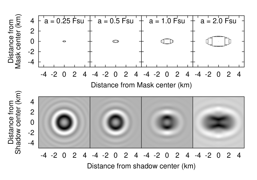
Figure 11.— Occulting masks (upper panels) and diffraction shadows (lower panels) for different-sized non-spherical KBOs (a/b=2.5 in each case, where a and b are the KBO’s semi-major and semi-minor axes.) The diffraction shadows are circularly symmetric for a$\lesssim$0.5 Fsu ($\sim$650m for visible light at 40 AU), despite the asymmetry of the occulting masks. The grayscales were chosen individually to cover the range of each shadow’s intensity.

Plant and recover tests were performed with profiles for 500 elliptical objects having uniformly distributed random parameters of: 200m$<a<$1000m, 0m$<$impact-parameter$<$4000m, 1.0$<(a/b)<$3.0, and $0<\theta<\pi$; where $a$, $b$, and $\theta$ are the semi-major and semi-minor axes of the object, and $\theta$ is the position angle of the rotated object. R_KBO was taken to be $0.5(a+b)$ in order to compare the results to Figure 7. The observed detection limits did not change and are shown in Figure 12. Thus, cross-correlation detection kernels based on circularly-symmetric occulting masks successfully detect occultations by sub-Fresnel-scale irregularly-shaped KBOs.

Figure 12.— The recovered sizes and impact parameters of planted occultation events for elliptical objects. Squares represent planted occultation events; filled if recovered, and open if not recovered. The 80% contour from the theoretical recovery tests for circular 40AU objects (Section 5.3) is shown with a solid line. The planted events had parameters of: 200m$<a<$1000m, 0m$<$impact-parameter$<$4000m, $1.0<(a/b)<3.0$, and $0<\theta<\pi$; where $a$, $b$, and $\theta$ are the semi-major and semi-minor axes of the object, and $\theta$ is the position angle of the rotated object. R_KBO was taken to be $0.5(a+b)$.

Our method of generating artificial time series did not incorporate the effects of variable noise levels in a time series. Although many of our recovery tests were performed with constant-noise artificial time series, they were verified in our final detection run by planting artificial occultation events in the real data. The results were found to be consistent with simulations we performed with the artificial data, and we believe that the presented estimates for the limiting detectable KBO size, $r_{min}$, and the maximum impact parameter, $b_{max}$, are accurate.

The presence of a period of increased noise within a time series alters the statistical properties of the variates. The overall measured standard deviation of the variates will lie between those measured for the low-noise and high-noise segments, which will lead to increases in the rates of false negatives and false positives in the respective segments. Our time series were broken into segments having approximately constant noise levels to mitigate this problem.

10. Summary

Analysis of our 5.0 star-hours of photometric time series on two B9V stars in the ecliptic open cluster, M35, revealed no viable candidate occultations. For the first time, the recovery of artificial occultation lightcurves was used to determine the limiting detectable object size and impact parameter for a KBO occultation. We place an upper limit on the surface density of KBOs of $\sum N(m_{R}<35.3)$ = $3.5\times 10^{10}$ deg^-2 (m${}_{R}\simeq$35.3 corresponds to a $\sim$860m (diameter) object with a geometric albedo of 0.04).

Having evaluated positive detections of TNO occultation events (Chang et al. 2006, 2007; Roques et al. 2006), we believe that the published events are likely to be spurious and that no serendipitous stellar occultation by a TNO has yet been reported. Comparison of the expected lightcurve structure for the C07 events with the observed structures show that the decreases in flux are too brief to be consistent with occultations by small bodies at 40 AU; and evaluation of the variability index, VI, used by R06 revealed that the VI variates are not normally distributed, but are drawn from a positively skewed distribution, prone to yielding high values. Also, the two $\sim$600m (diameter) TNOs discovered in 10 star-hours of R06 data suggest $\sim$4 such events should be present in the 89 star-hour x-ray time series observed at a similar ecliptic latitude ($\beta_{R06}=0.4\arcdeg S,\ 0.4\arcdeg S,\ 7.1\arcdeg N$, $\beta_{C06}=6\arcdeg N$). Nothing this large was reported by C06/C07.

Combining all results from the different surveys we place an overall 95%-confidence upper limit on the TNO surface density of: $\sum N(m_{R}<35.0)$ = $2.8\times 10^{9}$ deg^-2. A direct extrapolation of the observed CLF slope ($\alpha\approx$0.7) would yield a density of $\sum N(m_{R}<35.0)$ = $1.9\times 10^{8}$ deg^-2.

Our work is the first complete and careful examination of observational data for KBO occultations and their proper analysis and interpretation.

References

- Bailey (1976) Bailey, M. E. 1976, Nature, 259, 290
- Bernstein et al. (2004) Bernstein, G. M., Trilling, D. E., Allen, R. L., Brown, M. E., Holman, M., & Malhotra, R. 2004, AJ, 128, 1364
- Bertin & Arnouts (1996) Bertin, E. & Arnouts, S. 1996, A&AS, 117, 393
- Bickerton et al. (2006) Bickerton, S. J., Kavelaars, J., & Welch, D. L. 2006, American Astronomical Society Meeting Abstracts, 208, #76.03
- Bracewell (1986) Bracewell, R. 1986, The Fourier Transform and its Applications, 2nd edn. (New York: McGraw-Hill)
- Bradshaw et al. (2003) Bradshaw, C. F., Geldzahler, B. J., & Fomalont, E. B. 2003, ApJ, 592, 486
- Brown (2001) Brown, M. E. 2001, AJ, 121, 2804
- Brown et al. (2006) Brown, M. E., Schaller, E. L., Roe, H. G., Rabinowitz, D. L., & Trujillo, C. A. 2006, ApJ, 643, L61
- Brown & Webster (1997) Brown, M. J. I. & Webster, R. L. 1997, MNRAS, 289, 783
- Chang et al. (2006) Chang, H., King, S., Liang, J., Wu, P., Lin, L., & Chiu, J. 2006, Nature, 442, 850
- Chang et al. (2007) Chang, H.-K., Liang, J.-S., Liu, C.-Y., & King, S.-K. 2007, submitted MNRAS (astro-ph/0701850)
- Cooray (2003) Cooray, A. 2003, ApJ, 589, L97
- Cooray & Farmer (2003) Cooray, A. & Farmer, A. J. 2003, ApJ, 587, L125
- Cox (2000) Cox, A. N., ed. 2000, Allen’s Astrophysical Quantities, 4th edn. (New York: AIP Press; Springer)
- Davis & Farinella (1997) Davis, D. R. & Farinella, P. 1997, Icarus, 125, 50
- Dohnanyi (1969) Dohnanyi, J. W. 1969, J. Geophys. Res., 74, 2531
- Dyson (1992) Dyson, F. J. 1992, QJRAS, 33, 45
- Fraser et al. (2007) Fraser, W., Kavelaars, J., MacWilliams, J., Jones, L., Pritchet, C., Gladman, B., Holman, M., & Petit, J.-M. 2007, Accepted AJ
- Gaudi (2004) Gaudi, B. S. 2004, ApJ, 610, 1199
- Gladman et al. (1999) Gladman, B., Kavelaars, J. J., Morbidelli, A., Holman, M., Petit, J.-M., & Marsden, B. G. 1999, Minor Planet Electronic Circulars, 3
- Gladman et al. (2001) Gladman, B., Kavelaars, J. J., Petit, J.-M., Morbidelli, A., Holman, M. J., & Loredo, T. 2001, AJ, 122, 1051
- Jones et al. (2007) Jones, T. A., Levine, A. M., Morgan, E. H., & Rappaport, S. 2007, ArXiv Astrophysics e-prints, arXiv:astro-ph/07100837
- Jones et al. (2006) Jones, T. A., Levine, A. M., Morgan, E. H., & Rappaport, S. 2006, The Astronomer’s Telegram, 949, 1
- Jewitt et al. (1996) Jewitt, D., Luu, J., & Chen, J. 1996, AJ, 112, 1225
- Kenyon & Bromley (2004) Kenyon, S. J. & Bromley, B. C. 2004, AJ, 128, 1916
- Kenyon & Luu (1999a) Kenyon, S. J. & Luu, J. X. 1999a, AJ, 118, 1101
- Kenyon & Luu (1999b) —. 1999b, ApJ, 526, 465
- Kenyon & Windhorst (2001) Kenyon, S. J. & Windhorst, R. A. 2001, ApJ, 547, L69
- Kharchenko et al. (2004) Kharchenko, N. V., Piskunov, A. E., Röser, S., Schilbach, E., & Scholz, R.-D. 2004, Astron. Nachr., 325, 740
- Nihei et al. (2007) Nihei, T. C., Lehner, M. J., Bianco, F. B., King, S.-K., Giammarco, J. M., & Alcock, C. 2007, AJ, 134, 1596
- Pan & Sari (2005) Pan, M. & Sari, R. 2005, Icarus, 173, 342
- Roques et al. (2006) Roques, F., Doressoundiram, A., Dhillon, V., Marsh, T., Bickerton, S., Kavelaars, J. J., Moncuquet, M., Auvergne, M., Belskaya, I., Chevreton, M., Colas, F., Fernandez, A., Fitzsimmons, A., Lecacheux, J., Mousis, O., Pau, S., Peixinho, N., & Tozzi, G. P. 2006, AJ, 132, 819
- Roques & Moncuquet (2000) Roques, F. & Moncuquet, M. 2000, Icarus, 147, 530
- Roques et al. (1987) Roques, F., Moncuquet, M., & Sicardy, B. 1987, AJ, 93, 1549
- Sarajedini et al. (2004) Sarajedini, A., Brandt, K., Grocholski, A. J., et al. 2004, AJ, 127, 991
- Stern (1996) Stern, S. A. 1996, AJ, 112, 1203
- Stern & Colwell (1997) Stern, S. A. & Colwell, J. E. 1997, AJ, 114, 841
- Stern & McKinnon (2000) Stern, S. A. & McKinnon, W. B. 2000, AJ, 119, 945
- Sung & Bessell (1999) Sung, H. & Bessell, M. S. 1999, MNRAS, 306, 361