Multi-phase matching in the Grover algorithm

Abstract

Phase matching has been studied for the Grover algorithm as a way of enhancing the efficiency of the quantum search. Recently Li and Li found that a particular form of phase matching yields, with a single Grover operation, a success probability greater than 25/27 for finding the equal-amplitude superposition of marked states when the fraction of the marked states stored in a database state is greater than 1/3. Although this single operation eliminates the oscillations of the success probability that occur with multiple Grover operations, the latter oscillations reappear with multiple iterations of Li and Li’s phase matching. In this paper we introduce a multi-phase matching subject to a certain matching rule by which we can obtain a multiple Grover operation that with only a few iterations yields a success probability that is almost constant and unity over a wide range of the fraction of marked items. As an example we show that a multi-phase operation with six iterations yields a success probability between 99.8% and 100% for a fraction of marked states of 1/10 or larger.

I Introduction

The quantum search algorithm introduced by Grover Grover (1996, 1997a, 1997b, 2001) constitutes a major advance in quantum computing. It enables us to find a marked state stored in a database state consisting of $N$ unordered basis states in only ${\cal O}(\sqrt{N})$ Grover operations. A number of modifications and generalizations of the original Grover search algorithm have been proposed Grover (1998); Long et al. (1999, 2001); Collins (2002); Tulsi et al. (2006); Li and Li (2007); Younes (2007). In particular, phase matching methods in the Grover algorithm have been extensively examined Long et al. (1999, 2001); Li and Li (2007). The outcome of the search algorithm is characterized in terms of $P(\lambda)$, the probability of obtaining an equal-amplitude superposition of the marked states where $\lambda$ is the ratio of the marked states to all the states stored in the original database state.

Recently, Li and Li Li and Li (2007) proposed a new phase matching for the Grover algorithm and they obtained an improved success probability $P(\lambda)$ over a wide range of the ratio $\lambda$. They introduced the set of the Grover operators (details are described in Eqs. (1) and (2)): $U=I-(1-e^{i\alpha})\sum_{l=0}^{M-1}|t_{l}\rangle\langle t_{l}|$ and $V=Ie^{i\beta}+(1-e^{i\beta})|0^{\otimes n}\rangle\langle 0^{\otimes n}|$. The phase factor $e^{i\beta}$ in the first term of the operator $V$ was first introduced in Ref. Li and Li (2007). In the new phase matching the number of phases is the same as the usual one but the form of the phase shift operator $V$ is different. Li and Li found the remarkable result that a single Grover operation of the new phase matching yields $P(\lambda)>25/27$ for $1/3\leq\lambda\leq 1$. This is significant in the sense that with only one Grover operation the efficiency of the Grover algorithm is substantially improved in the range of values of $\lambda$ where the efficiency of the original algorithm deteriorates.

This phase matching has another interesting aspect that was not explicitly pointed out by Li and Li Li and Li (2007). For a given values of $\lambda$ in the range $1/4\leq\lambda\leq 1$, one Grover operation with the phases $\alpha=-\beta=\arccos(1-1/2\lambda)$ yields exactly $P=1$. [See Eq. (11) in the following.] This results was obtained earlier by Chi and Kim Chi and Kim (1997) who considered a modified Grover operator of arbitrary phase. The special case of $\lambda=1/2$ yields $\alpha=-\beta=\pm\pi/2$, which are the phases found in Ref. Li and Li (2007). This aspect of the phase matching is also significant because it implies that one can always find the equal-amplitude superposition of the marked states by only one Grover operation when $\lambda$ is greater than 1/4 by tuning the phases $\alpha$ and $\beta$ appropriately for the given $\lambda$. Conditions for a success probability of unity have been studied by previous authors. See, for example, Refs. Høyer (2000); Long (2001).

It should be pointed out, however, that the so-called new phase matching of Ref. Li and Li (2007) is equivalent to the original phase matching of Long et al. Long et al. (1999). When the second operator is defined as $V^{\prime}=e^{-i\beta}V$, it becomes the phase-matching operator of Long et al. The only difference between the two is that the overall state is multiplied by a phase factor and so the amplitudes of the components are different, but the probabilities are the same. Thus the remarkable result of Li and Li can also be seen to follow from the operator of Long et al. Analytically the formulation by Li and Li is somewhat more transparent and hence we use it throughout this paper, except in the Appendix where we explicitly show the equivalence of the two formulations by calculating the probability profile.

Thus a number of aspects of the Grover algorithm with phase matching, already alluded to, are of particular interest and they form the objectives of this study. We focus on high success probabilities with as few iterations as possible in order to enhance the efficiency of the quantum search. We emphasize the following three objectives: (1) the elucidation of features of the phase-matched Grover operations with a small number of iterations that yield success probabilities $P(\lambda)$ close to one over a wide range of values of $\lambda$, (2) given a value of $\lambda$ the determination of the phase-matched Grover operator(s) that results in $P(\lambda)=1$ exactly, and (3) the elucidation of the features of the phase-matched Grover operators that allow us to obtain $P(\lambda)=1$ for very small values of $\lambda$.

In this paper we explore the search algorithm with these objectives in mind using the advantages of a few multiple Grover operations with phase matching. It is well known that a multiple application of the original Grover operation gives rise to intensive oscillations of $P$ as a function of $\lambda$ and such oscillations deteriorate the efficiency of the algorithm. This undesirable feature remains even in the new phase matching of Li and Li, as we will illustrate. We show that if we introduce a multi-phase matching subject to a certain matching rule, we can obtain a multiple Grover operation that yields a success probability almost constant and unity over a wide range of $\lambda$, e.g., $0.1\leq\lambda\leq 1$. This is also significant in the sense that when $\lambda$ is greater than a small minimum value we can always find the superposition of the marked states with high degree of certainty without (re)tuning the phases.

In the next section we set up the algorithm of the multi-phase matching in the framework of the phase matching of Li and Li Li and Li (2007) and analyze the efficiency of the algorithm by considering a single matched phase and a two-stage multi-phase matching. We also obtain an exemplar of a good probability profile for a six-stage multi-phase matched operator. In Sec. III we consider the success probability for small $\lambda$ by using the Grover operations with a phase other than $\pi$. We summarize our results in Sec. IV.

II Multi-phase matching in the framework of the new phase matching

The new phase matching in the Grover algorithm proposed by Li and Li Li and Li (2007) is defined with the two operators,

$$U=I-(1-e^{i\alpha})\sum_{l=0}^{M-1}|t_{l}\rangle\langle t_{l}|$$ (1)

$$V=Ie^{i\beta}+(1-e^{i\beta})|0^{\otimes n}\rangle\langle 0^{\otimes n}|.$$ (2)

where $|0^{\otimes n}\rangle$ is the $n$-qubits initial state, $M$ is the number of target (marked) states stored in an unstructured database state, and the $|t_{l}\rangle$ denote the target or marked states. The database state is given as $|\phi\rangle=H^{\otimes n}|0^{\otimes n}\rangle$, where $H$ is the Walsh-Hadamard transformation. The state $|\phi\rangle$ is an equally-weighted superposition of the $N=2^{n}$ basis states, $|w_{l}\rangle,\ l=0,\dots,N-1$. The fraction $\lambda$ of the target states is defined as $\lambda=M/N$. The $U$ and $V$ of Eqs. (1) and (2) are both unitary as was shown in Ref. Li and Li (2007). With $\alpha=\beta=\pi$, $U$ and $V$ reduce to the Grover operators of the original algorithm. As we mentioned in Sec. I, Li and Li showed explicitly that a single Grover operation of the new phase matching $(H^{\otimes n}VH^{\otimes n})UH^{\otimes n}|0^{\otimes n}\rangle$ with $\alpha=-\beta=\pi/2$ yields a success probability $P(\lambda)>25/27$ for $1/3\leq\lambda\leq 1$.

We introduce a multi-phase matching within the framework of the new phase matching. We rewrite the database state $|\phi\rangle=H^{\otimes n}|0^{\otimes n}\rangle=N^{-1/2}\sum_{l=0}^{N-1}|\omega_{l}\rangle$ in terms of $\lambda$ as

$$|\phi\rangle=\frac{1}{\sqrt{N}}\sum_{l=0}^{N-1}|\omega_{l}\rangle = \sqrt{\frac{N-M}{N}}|R\rangle+\sqrt{\frac{M}{N}}|T\rangle$$ (3)

$$= \sqrt{1-\lambda}|R\rangle+\sqrt{\lambda}|T\rangle,$$

where

$$|R\rangle=\frac{1}{\sqrt{N-M}}\sum_{l=0}^{N-M-1}|r_{l}\rangle,\ \ |T\rangle=\frac{1}{\sqrt{M}}\sum_{l=0}^{M-1}|t_{l}\rangle.$$ (4)

The state $|T\rangle$ is the uniform superposition of the marked states and $|R\rangle$ is that of the remaining states $|r_{l}\rangle$. They are both normalized to unity and orthogonal to each other. In the following, for convenience, we work in the two-dimensional space defined by the basis $\{|R\rangle,|T\rangle\}$. The two-dimensional representations of $U$ and $H^{\otimes n}VH^{\otimes n}=Ie^{i\beta}+(1-e^{i\beta})|\phi\rangle\langle\phi|$ are

$$U:\begin{pmatrix}1&0\\ 0&e^{i\alpha}\end{pmatrix},\ \ \ H^{\otimes n}VH^{\otimes n}:\begin{pmatrix}(1-e^{i\beta})(1-\lambda)+e^{i\beta}&(1-e^{i\beta})\sqrt{\lambda(1-\lambda)}\\ (1-e^{i\beta})\sqrt{\lambda(1-\lambda)}&(1-e^{i\beta})\lambda+e^{i\beta}\end{pmatrix}.$$ (5)

We write the multiple Grover operation with the multiple phases $\alpha_{j}$ and $\beta_{j}$ $(j=1,\dots,k)$ as

$$\begin{pmatrix}u_{k}\\ d_{k}\end{pmatrix}=G(\alpha_{k},\beta_{k})G(\alpha_{k-1},\beta_{k-1})\cdots G(\alpha_{1},\beta_{1})\begin{pmatrix}\sqrt{1-\lambda}\\ \sqrt{\lambda}\end{pmatrix},$$ (6)

where one Grover operation $G(\alpha_{j},\beta_{j})$ $(j=1,\dots,k)$ in this representation is

$$G(\alpha_{j},\beta_{j})=\begin{pmatrix}(1-e^{i\beta_{j}})(1-\lambda)+e^{i\beta_{j}}&(e^{i\alpha_{j}}-e^{i(\alpha_{j}+\beta_{j})})\sqrt{\lambda(1-\lambda)}\\ (1-e^{i\beta_{j}})\sqrt{\lambda(1-\lambda)}&(e^{i\alpha_{j}}-e^{i(\alpha_{j}+\beta_{j})})\lambda+e^{i(\alpha_{j}+\beta_{j})}\end{pmatrix}.$$ (7)

The success probability of finding the superposition of target states is given by $P_{k}(\lambda)\equiv|d_{k}|^{2}$.

We now consider the one- and two-pair-phase cases before increasing the phase-matching to six different pairs of phases in order to obtain $P(\lambda)$ nearly equal to unity over a large range of values of $\lambda$. In other words, we discuss the $k=1$ and the $k=2$ cases in detail first, and then proceed to the numerical results of the $k=6$ case.

II.1 Multi-phase matching with one pair of phases

When $k=1$, Eq. (6) reduces to

$$\begin{pmatrix}u_{1}\\ d_{1}\end{pmatrix}=G_{1}(\alpha,\beta)\begin{pmatrix}\sqrt{1-\lambda}\\ \sqrt{\lambda}\end{pmatrix}.$$ (8)

Since we first focus on cases of complete success $P=|d_{1}|^{2}=1-|u_{1}|^{2}=1$, we can equivalently consider the condition $u_{1}=0$. In general

$$u_{1}=\sqrt{1-\lambda}\,[1-\lambda+e^{i\beta}\lambda+(e^{i\alpha}-e^{i(\alpha+\beta)})\lambda\,].$$ (9)

The condition that $u_{1}$ be zero leads to

$$\frac{1}{\lambda} = 1-\cos\alpha-\cos\beta-\cos(\alpha+\beta)$$ (10)

$$\ \ +i[\sin{(\alpha+\beta)}-\sin\alpha-\sin\beta].$$

The fact that $\lambda$ must be real implies that (1) $\beta=-\alpha$, (2) either $\alpha$ or $\beta$ are zero, or (3) both $\alpha$ and $\beta$ are zero. When $\beta=0$ in the operator $V$ of Eq. (2), the operator is the identity and the overall effect of operator $U$ of Eq. (1) by itself would cause the phase of the marked states to be changed, but the probabilities of marked and unmarked states would remain the same. When $\alpha=0$, then $U=I$ and $G=H^{\otimes n}VH^{\otimes n}$. The initial state $|\phi\rangle$ is an eigenvector of $G$ with eigenvalue 1. Thus $G$ does not cause any evolution in $|\phi\rangle$. The success probability is $P=\lambda$, which is the success probability of the classical algorithm. As no quantum improvement to the search algorithm is achieved, we eliminate the case of $\alpha=0$ and any nonzero $\beta$ from the solutions of Eq. (10). Thus only the solution $\beta=-\alpha$ is meaningful, and yields, as mentioned in Sec. I and in Ref. Chi and Kim (1997), $P=1$ when

$$\alpha=-\beta=\arccos(1-1/2\lambda).$$ (11)

Since $\lambda$ lies between zero and one, the range of $\alpha$ is $\pi/3\leq\alpha\leq\pi$. The boundary point of this range $\alpha=\pi/3$ occurs when $P(\lambda=1)=1$, and similarly $\alpha=\pi$ when $P(\lambda=1/4)=1$.

We can express $P(\lambda)$ as a function of $\lambda$ depending on the parameter $\alpha$,

$$P(\lambda) = 1-|u_{1}|^{2}$$ (12)

$$= \lambda\,[5-4\,\cos\alpha-4\,(1-\cos\alpha)\,(2-\cos\alpha)\,\lambda$$

$$\ \ \ \ +4\,(1-\cos\alpha)^{2}\lambda^{2}].$$

For $\alpha=\pi/2$ the equation reduces to Eq. (14) of Li and Li Li and Li (2007) . Since Eq. (12) is cubic in $\lambda$ we expect a local maximum and a local minimum in the range $0<\lambda\leq 1$ at $\lambda_{\mathrm{max}}$ and $\lambda_{\mathrm{min}}$ respectively, where

$$\lambda_{\mathrm{max}}=\frac{1}{2\,(1-\cos\alpha)},\ \ \lambda_{\mathrm{min}}=\frac{5-4\cos\alpha}{6\,(1-\cos\alpha)}.$$ (13)

Furthermore the extrema are

$$P(\lambda_{\mathrm{max}})=1,\ \ P(\lambda_{\mathrm{min}})=\frac{(1+\cos\alpha)(5-4\cos\alpha)^{2}}{27\,(1-\cos\alpha)}.$$ (14)

We illustrate different cases in Fig. 1.

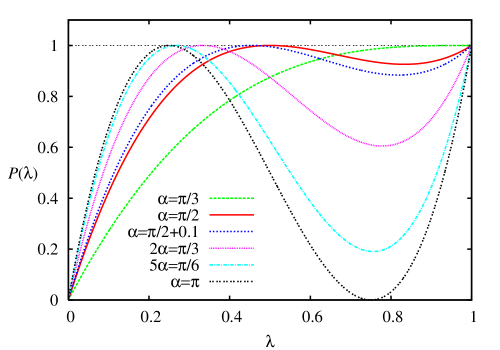
Figure 1: (Color online) Plots of $P(\lambda)$ for different values of the parameter $\alpha$ for the case of one iteration. (See Eq. (12).)

It is evident that the $\alpha=\pi/2$ case, which is the one used by Li and Li Li and Li (2007), gives the optimal profile for the success probability. Optimal here could be defined as the largest average $P$ over the range of $\lambda$, or the largest range of $\lambda$ over which $P\geq 25/27$.

II.2 Multi-phase matching with two pairs of phases

We now consider Eq. (6) for $k=2$ and we again concentrate on the upper component of the vector $(u_{2},d_{2})^{T}$. The general expression for it is too lengthy to give here, but again we demand that for an arbitrary value of $\lambda$ the imaginary part is zero to obtain the matching relationship for the phases. Apart from a factor of $\sqrt{1-\lambda}$ the expression of $\mathrm{Im}\,u_{2}$ contains a term in $\lambda$ and another in $\lambda^{2}$. Demanding that the coefficients of each power of $\lambda$ vanishes gives us two equations involving $\alpha_{1}$, $\alpha_{2}$, $\beta_{1}$, and $\beta_{2}$. Solving for $\beta_{1}$ and $\beta_{2}$ in terms of $\alpha_{1}$ and $\alpha_{2}$ we obtain the following four solutions:

$$\left.\begin{array}[]{l}\{\beta_{1}=-\alpha_{1},\ \beta_{2}=0\}\\ \{\beta_{1}=-\alpha_{2},\ \beta_{2}=-\alpha_{1}\}\\ \{\beta_{1}=\beta_{2}=0\}\\ \{\beta_{1}=0,\ \beta_{2}=-(\alpha_{1}+\alpha_{2})\}.\end{array}\right.$$

Since one of $\beta_{1}$ and $\beta_{2}$ is zero for the first and last solution, the operation is then reduced to one iteration, and for the third solution the two iterations would not change the probabilities of the marked and unmarked states. Thus the only solution that gives new information is the one where $\beta_{1}=-\alpha_{2}$ and $\beta_{2}=-\alpha_{1}$. (The fact that $\mathrm{Im}\,u_{2}=0$ is a necessary, but not a sufficient, condition for this solution.) After obtaining the matched phases for which $\mathrm{Im}\,u_{2}=0$, we set $\mathrm{Re}\,u_{2}=0$ to solve for the values of $\lambda$ which gives $P=1$.

The expression for $u_{2}$ is then real and can be written as

$$u_{2} = \{1+2\,[(1-\cos\alpha_{1})(-2+\cos\alpha_{2})-\sin\alpha_{1}\sin\alpha_{2}]\,\lambda$$ (15)

$$+4\,(1-\cos\alpha_{1})(1-\cos\alpha_{2})\,\lambda^{2}\}\sqrt{1-\lambda}.$$

The factor multiplying $\sqrt{1-\lambda}$ is quadratic in $\lambda$ and hence it can vanish for two values of $\lambda$. Thus we can ask ourselves the questions, suppose two values of $\lambda$ between zero and one are given at which $P(\lambda)=1$, what are the corresponding values of $\alpha$ and what limits are there on the possible values of $\lambda$ that satisfy $P(\lambda)=1$? If $\lambda_{1}$ and $\lambda_{2}$ are the roots of the equation

$$u_{2}(\lambda)/\sqrt{1-\lambda}=0,$$ (16)

then $\cos\alpha_{1}$ and $\cos\alpha_{2}$ satisfy the equations

$$8\lambda_{1}\lambda_{2}\cos^{3}\alpha_{2}+[4(\lambda_{1}+\lambda_{2})(1-\lambda_{1}-\lambda_{2})-8\lambda_{1}\lambda_{2}]\cos^{2}\alpha_{2}+[8(\lambda_{1}+\lambda_{2})^{2}-12(\lambda_{1}+\lambda_{2})-8\lambda_{1}\lambda_{2}+4]\cos\alpha_{2}$$

$$\hskip 122.85876pt-4(\lambda_{1}+\lambda_{2})^{2}+8(\lambda_{1}+\lambda_{2})-5+8\lambda_{1}\lambda_{2}=0,$$ (17)

$$\cos\alpha_{1}=1-\frac{1}{4(1-\cos\alpha_{2})\lambda_{1}\lambda_{2}}.$$ (18)

In order to have a sense of the values of $\alpha_{1}$ and $\alpha_{2}$ that are valid, we have minimally the condition that the discriminant of Eq. (16) (quadratic in $\lambda$) should be nonnegative to avoid complex values of $\lambda$. In Fig. 2 we plot the discriminant as a surface $z=D(\alpha_{1},\alpha_{2})$; the intersection of the surface with the $xy$ plane gives the boundary of the non-allowed $\alpha_{1}$ and $\alpha_{2}$ values.

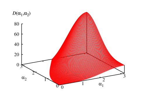
Figure 2: (Color online) The discriminant of Eq. (16) as a function of $\alpha_{1}$, and $\alpha_{2}$. The curve of intersection of the surface with the $D=0$ plane separates the smaller values of $\alpha_{1}$ for which there are no physical operators.

Given $\lambda_{1}$ and $\lambda_{2}$ one can solve Eq. (II.2) for $\cos\alpha_{2}$ and using it we obtain $\cos\alpha_{1}$ from the second equation. Only those solutions that yield real angles $\alpha_{1}$ and $\alpha_{2}$ are meaningful for the unitary operators. The minimum value of $\lambda$ for which $P=1$ occurs when $\alpha_{1}=\alpha_{2}=\pi$. In that case $\lambda=(3-\sqrt{5})/8=0.09549$. It can be shown that varying $\alpha_{1}$ or $\alpha_{2}$ by a small amount away from $\pi$ always leads to an increase in the $\lambda$ which corresponds to the smaller of the two values of $\lambda$. When we let $\alpha_{1,2}=\pi+\epsilon_{1,2}$ we obtain a change in the smaller $\lambda$ of

$$\Delta\lambda=\frac{1}{160}\left[\left(2\sqrt{5}\epsilon_{1}+\frac{5-3\sqrt{5}}{\sqrt{2\sqrt{5}}}\epsilon_{2}\right)^{2}+(22-8\sqrt{5})\epsilon_{2}^{2}\right],$$ (19)

which is positive regardless of the signs of $\epsilon_{1,2}$. The larger $\lambda$ can increase or decrease with changes in the phases(s).

We obtain a particular example using the procedure described above. We search through combinations of $\lambda_{1,2}$ and find that $\lambda_{1}=2/5$ and $\lambda_{2}=4/5$ give good results. In this case $\alpha_{1}=1.00889485$ and $\alpha_{2}=2.30794928$. We find local minima of $P(\lambda)$ at $\lambda=0.5767$ and $\lambda=0.9433$ at which $P=0.9936$ and 0.9966, respectively. The corresponding graph of the success probability as a function of $\lambda$ obtained with the two-stage multi-phase operator is shown in Fig. 3 and compared with double iterations of the Grover operation and that of Li and Li Li and Li (2007).

It would be interesting to examine a classical counterpart of $P(\lambda)$. The probability of failing to find one of $M$ marked objects out of $N$ objects is $(N-M)/N=1-\lambda$. The probability of failing twice in a row is

$$(1-\lambda)\left(\frac{N-1-M}{N-1}\right)=(1-\lambda)\left(1-\frac{\lambda}{1-1/N}\right).$$

The probability of failing $k$ times in a row is

$$(1-\lambda)\left(1-\frac{\lambda}{1-1/N}\right)\cdots\left(1-\frac{\lambda}{1-(k-1)/N}\right)$$

$$=\prod_{n=1}^{k}\left[1-\lambda\left(1-\frac{n-1}{N}\right)^{-1}\right].$$

Thus the probability of finding at least one of the $M$ items in $k$ successive attempts is

$$P_{\mathrm{classical}}(\lambda)=1-\prod_{n=1}^{k}\left[1-\lambda\left(1-\frac{n-1}{N}\right)^{-1}\right].$$ (20)

If $k\ll N$, this probability is approximately $P_{\mathrm{classical}}(\lambda)\approx 1-(1-\lambda)^{k}$, which we interpret as the classical counterpart of $P(\lambda)$. This probability with $k=2$ is also plotted in Fig. 3.

Figure 3: (Color online) Plots of $P(\lambda)$ obtained after two iterations of the multiphase case with $\alpha_{1}=1.00889485$ and $\alpha_{2}=2.30794928$. For comparison the double Grover iteration ($\alpha_{1}=\alpha_{2}=\pi$), the double iteration of Li and Li ($\alpha_{1}=\alpha_{2}=\pi/2$), and the classical counterpart are shown as well.

II.3 Multi-phase matching with six pairs of phases

We show that if we match the multi-phase $\alpha_{j}$ and $\beta_{j}$ $(j=1,\dots,k)$ with $k=6$ in accordance with a certain matching rule (best fit), we can obtain a multiple Grover operation that yields $P(\lambda)\approx 1$ in a wide range of $\lambda$. We found this best solution for six Grover iterations by a nonlinear fitting to the ideal probability curve $P(\lambda)=1$ for $0<\lambda\leq 1$. The phases $\alpha_{j}$ and $\beta_{j}$ found in this way are given in the left side of Table 1.

$~{}~{}j~{}~{}$	$\alpha_{j}/\pi$	$\beta_{j}$	$\lambda_{j}^{(P(\lambda_{j})=1)}$	$P(\lambda_{j}^{(\mathrm{local~{}min})})$
1	1.20560132	$-\alpha_{6}$	0.10777	0.9980
2	1.29806396	$-\alpha_{5}$	0.23793	0.9993
3	1.31701508	$-\alpha_{4}$	0.41889	0.9996
4	1.33356767	$-\alpha_{3}$	0.62393	0.9997
5	0.47289426	$-\alpha_{2}$	0.81366	0.9997
6	1.66668634	$-\alpha_{1}$	0.94483	0.9995

Table 1: Phase parameters for the six-parameter multi-phase matching, and results for local maxima ($P(\lambda)=1$) and local minima of $P(\lambda)$.

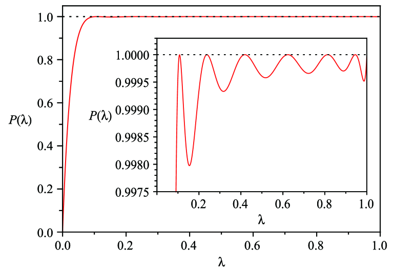
Figure 4: (Color online) Success probability curves $P(\lambda)$ obtained with the multi-phase matching with six iteration in the operation. The phase parameters are given in the left side of Table 1.

It is remarkable that $\alpha_{j}$ and $\beta_{j}$ are matched to each other such that $\alpha_{j}=-\beta_{6-j+1}$. The signs of $\alpha_{j}$ and $\beta_{j}$ are opposite to each other, which is consistent with the case of the new phase matching of Ref. Li and Li (2007), i.e., the $k=1$ case with $\alpha_{1}=-\beta_{1}=\pi/2$. The matching rule $\alpha_{j}=-\beta_{k-j+1}$ between the multi-phases $\alpha_{j}$ and $\beta_{j}$ holds for any $k$ in the best solution obtained by the nonlinear fitting to the ideal probability curve $P(\lambda)=1$ for $0<\lambda\leq 1$, although we omit to show cases other than those for which $k=1$, 2, and 6.

Fig. 4 shows the success probabilities obtained by six Grover operations with the multi-phase matching of Eq. (6). The inset of Fig. 4 shows that there are six values of $\lambda_{i}$ at which $P(\lambda_{i})=1$ exactly. They are given in the right side of Table 1 along with local minimum values of the function $P(\lambda)$ which occur between 0.1 and 1.

We studied the $k=5$ case in the same way and obtained a graph similar to Fig. 4 with $P(\lambda)=1$ for five values of $\lambda$ other than unity. The local minima of $P(\lambda)$ are lower and the minimum value of $\lambda$ for which $P(\lambda)=1$ is slightly larger than in the $k=6$ case. The matching rule $\alpha_{j}=-\beta_{k-j+1}$ is also satisfied for the $k=5$ case as it was for $k=1$, 2, and 6 cases. We are confident that for any $k>1$ this matching rule for the best fit holds so that in general one finds $k$ values of $\lambda$ for which $P(\lambda)=1$ and the smallest $\lambda$ for which $P(\lambda)=1$ decreases as $k$ increases.

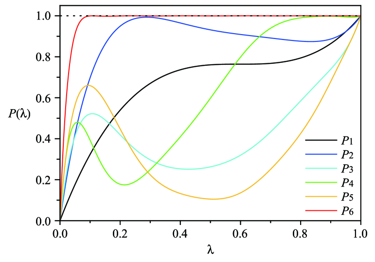
Figure 5: (Color online) Success probability curves $P_{i}(\lambda)$ at the $i$th stage obtained with the six-stage multi-phase matching. The phase parameters are given in the left side of Table 1.

Returning to the six-stage multiple phase operation, we define $P_{j}(\lambda)$ $(j=1,\dots,6)$ as the success probability curves after $j$ steps of the six-stage multi-phase operation. As seen in the Figs. 4 and 5, $P_{6}(\lambda)\approx 1$ is achieved for $0.1\leq\lambda\leq 1$ in the sixth Grover operation. This is significant in the sense that if $\lambda$ is greater than 0.1, we can always find the superposition of marked states by just six Grover operations. In contrast to the shape of the curve for $P_{6}(\lambda)$, Fig. 5 shows that each $P_{j}(\lambda)$ for $j=1,\dots,5$ depends strongly on $\lambda$ and is far from the desired success probability $P_{6}(\lambda)$. The curves do not monotonically approach the desired success probability $P_{6}(\lambda)$ when $\lambda>0.05$. In particular, $P_{5}(\lambda)$ is quite different from the desired probability $P_{6}(\lambda)$. However, in the final (sixth) step the desired probability $P_{6}(\lambda)$ is obtained. This is in contrast to the fixed-point iteration schemes studied in Refs. Grover (2005); Tulsi et al. (2006); Younes (2007).

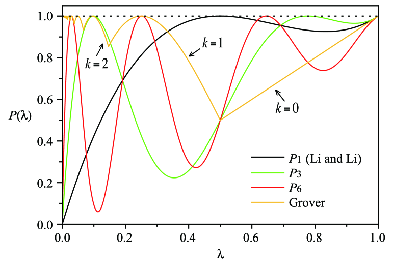
Figure 6: (Color online) Success probability curves $P_{1}(\lambda)$, $P_{3}(\lambda)$, and $P_{6}(\lambda)$ obtained with the single phase matching with $\alpha_{j}=-\beta_{j}=\pi/2$ $(j=1,\cdots,6)$. The $P_{1}(\lambda)$ indicates the success probability of the new phase matching of Ref. Li and Li (2007). The yellow curve is the success probability of the original Grover’s algorithm, where the graph segments are plotted for optimal iteration times indicated by $k$. Iteration times for small $\lambda$ are omitted.

Figure 6 shows the success probabilities obtained by six Grover operations with the single phase matching with $\alpha_{j}=-\beta_{j}=\pi/2$ $(j=1,\dots,6)$ , where we showed only $P_{1}(\lambda)$, $P_{3}(\lambda)$ and $P_{6}(\lambda)$. The $P_{1}(\lambda)$ is the success probability of the new phase matching obtained by Li and Li Li and Li (2007). As stressed in Ref. Li and Li (2007), the success probability is substantially improved in $\lambda>1/3$ by a single Grover operation, compared with that of the original Grover algorithm indicated by the yellow line, where the probability is plotted for optimal iteration times indicated by $k$. However, $P_{3}(\lambda)$ and $P_{6}(\lambda)$ obtained by multiple Grover operations with the single phase matching show intensive oscillations with $\lambda$. As we have shown, such undesirable oscillations can be eliminated by the multi-phase matching subject to the matching rule $\alpha_{j}=-\beta_{6-j+1}$.

Here we should note that the nonlinear fitting is not unique. The phases $\alpha_{j}$ and $\beta_{j}$ given in Table 1 were obtained by minimizing the function $\sum_{i}\chi_{i}^{2}$ where the $\chi_{i}$ are the differences at $\lambda=\lambda_{i}$ of the ideal probability $P(\lambda)=1$ and the probability function $P_{6}(\lambda)$. If we take, for example, a function such as $\sum_{i}|\chi_{i}|$ we obtain another solution. Although this solution gives almost the same $P_{6}(\lambda)$, the probability curve is shifted slightly toward larger values of $\lambda$, so that the local extrema are also slightly moved to the right. Since we emphasize obtaining $P(\lambda)\approx 1$ over as wide a range of $\lambda$ as possible we adopted the solution that uses the $\chi^{2}_{i}$ for the fitting.

III Iteration of Grover’s operation with phase other than $\pi$

In this section we consider the repeated application of Grover’s original operation generalized to have a phase other than $\pi$. We focus in particular on cases with small $\lambda$ for which the success probability with the multi-phase matching is small, and determine the conditions that yield success probabilities close to unity.

Consider a single Grover operation with matched phase, Eq. (7), but with $\beta=-\alpha$,

$$G_{1}=\begin{pmatrix}(1-e^{-i\alpha})(1-\lambda)+e^{-i\alpha}&(e^{i\alpha}-1)\sqrt{\lambda(1-\lambda)}\\ (1-e^{-i\alpha})\sqrt{\lambda(1-\lambda)}&(e^{i\alpha}-1)\lambda+1\end{pmatrix}.$$ (21)

Note that $\det G_{1}=1$. We obtain eigenvalues $\sigma$ of the matrix $G_{1}$ by solving

$$f(\sigma)=\det(G_{1}-\sigma I)=0.$$ (22)

The characteristic function $f(\sigma)$ is

$$f(\sigma)=\sigma^{2}+2[-1+(1-\cos\alpha)\lambda]\sigma+1.$$ (23)

The equation $f(\sigma)=0$ yields solutions

$$\sigma=1-(1-\cos\alpha)\lambda\pm i\sqrt{(1-\cos\alpha)\lambda[2-(1-\cos\alpha)\lambda]}$$ (24)

We define $x$ as

$$x=(1-\cos\alpha)\lambda,$$ (25)

so that the eigenvalues can be written as

$$\sigma=e^{\pm i\phi},\ \ \phi=\arctan\left(\frac{\sqrt{x(2-x)}}{1-x}\right).$$ (26)

We choose the definition of the arc tangent so that as $x$ varies from 0 to 2, $\phi$ goes from 0 to $\pi$. We can rewrite the function $f(\sigma)$ as

$$f(\sigma)=\sigma^{2}-2\sigma\cos\phi+1.$$ (27)

By the Cayley-Hamilton theorem (Pipes, 1958, page 91) $f(G_{1})=0$, so that we obtain the identity

$$G_{1}^{2}=2G_{1}\cos\phi-1.$$ (28)

This means that $G_{1}$ iterated any number of times can be written as a linear expression of $G_{1}$. In fact for $k$ iterations it can be shown by induction Sprung et al. (1993) that

$$G_{1}^{k}=\frac{1}{\sin\phi}\left[G_{1}\sin(k\phi)-\sin((k-1)\phi)\right].$$ (29)

Consider now the $k$ iterations of the Grover operation, so that

$$\begin{pmatrix}u_{k}\\ d_{k}\end{pmatrix}=G_{1}^{k}\begin{pmatrix}\sqrt{1-\lambda}\\ \sqrt{\lambda}\end{pmatrix}.$$ (30)

This yields

$$\begin{pmatrix}u_{k}\\ d_{k}\end{pmatrix}=\frac{1}{\sin\phi}\left[\sin{(k\phi)}\begin{pmatrix}(1-e^{-i\alpha})(1-\lambda)+e^{-i\alpha}&(e^{i\alpha}-1)\sqrt{\lambda(1-\lambda)}\\ (1-e^{-i\alpha})\sqrt{\lambda(1-\lambda)}&(e^{i\alpha}-1)\lambda+1\end{pmatrix}-\sin{((k-1)\phi)}\ I\right]\begin{pmatrix}\sqrt{1-\lambda}\\ \sqrt{\lambda}\end{pmatrix}.$$ (31)

Thus the expression for $u_{k}$ is

$$u_{k}=\frac{\sqrt{1-\lambda}}{\sin\phi}\left\{\sin{(k\phi)}(1-2x)-\sin{((k-1)\phi)}\right\}.$$ (32)

We require $u_{k}=0$ so that $P=1$. A trivial solution is $\lambda=1$. We also note that $\phi=0$ yields $x=-1/(2k)$. Since $x$ must be positive $\sin{\phi}\neq 0$. Thus we need to solve only

$$\sin{(k\phi)}(1-2x)-\sin{((k-1)\phi)}=0.$$ (33)

The solutions are values of $x=(1-\cos{\alpha})\lambda$ for which $P=1$. Thus we have $P=1$ for combinations of $\alpha$ and $\lambda$. For instance, when $\alpha=\pi$, then $\lambda=x/2$. In Fig. 7, we display the $P(\lambda)$ curves for six ($k=6$) iterations when $\alpha$ has different values.

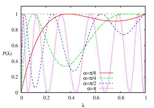
Figure 7: (Color online) Plots of $P(\lambda)$ obtained after six iterations with a single $\alpha$ for the cases of $\alpha=\pi/8,\ \pi/4,\ \pi/2$, and $\pi$.

For large $k$ we can estimate the smallest value of $\lambda$ for which $P$ is unity. We rewrite Eq. (33) so that

$$\tan(k\phi)=\frac{\sin\phi}{\cos\phi-1+2x}.$$ (34)

The value of $x$ which is the solution occurs for the $x$ coordinate of the point of intersection of the curves represented by the left side and the right side of Eq. (34). The curve on the right is a smoothly decreasing positive function starting at infinity when $x=0$ and asymptotically approaching the positive $x$ axis. The curve on the left starts at zero and increases to positive infinity when $k\phi=\pi/2$. When $k$ is large this occurs for small values of $\phi$ or small values of $x$. Thus using the condition $\phi\approx\pi/(2k)$, we obtain

$$\arctan\frac{\sqrt{x(2-x)}}{1-x}\mathrm{\raisebox{-2.58334pt}{$\stackrel{{\scriptstyle\textstyle<}}{{\sim}}$}}\frac{\pi}{2k}\ \ \mathrm{or}\ \ \frac{\sqrt{x(2-x)}}{1-x}\mathrm{\raisebox{-2.58334pt}{$\stackrel{{\scriptstyle\textstyle<}}{{\sim}}$}}\frac{\pi}{2k}.$$ (35)

This leads to the approximation of the smallest value of $x$ for which $P$ is one as $x_{\mathrm{min}}\mathrm{\raisebox{-2.58334pt}{$\stackrel{{\scriptstyle\textstyle<}}{{\sim}}$}}\pi^{2}/(8k^{2})$; for $\alpha=\pi$ (the Grover case) $\lambda_{\mathrm{min}}=x_{\mathrm{min}}/2$. This approximation leads to $\lambda_{\mathrm{min}}=0.017$ for $k=6$ and $\alpha=\pi$, whereas the exact solution of Eq. (34) gives $0.014$. As $k$ gets larger the approximation improves further.

III.1 The Grover algorithm as a special case

We recover the Grover algorithm starting with Eq. (32) and setting $\alpha=\pi$ or $x=2\lambda$. Then it follows from Eq. (26) that $\sin\phi=\sqrt{4\lambda(1-\lambda)}$ and $\cos\phi=(1-2\lambda)$. The $u_{k}$ of Eq. (32) can be reduced to

$$u_{k}=-\sqrt{\lambda}\sin(k\phi)+\sqrt{1-\lambda}\cos(k\phi).$$ (36)

Define $\sin\theta=\sqrt{\lambda}$. Then

$$u_{k}=\cos(k\phi+\theta).$$ (37)

We can show that $\phi=2\theta$, so that

$$u_{k}=\cos[(2k+1)\theta]=\cos[(2k+1)\arcsin(\sqrt{\lambda})].$$ (38)

This is Eq. (6) of Ref. Li and Li (2007). Furthermore

$$P=1-u_{k}^{2}=\sin^{2}[(2k+1)\arcsin(\sqrt{\lambda})].$$ (39)

Thus each iteration effectively rotates the state through an angle of $\theta/2=\arcsin(\sqrt{\lambda})/2$. We can use this to estimate the number of iterations that are required to obtain $P(\lambda)=1$. That occurs when the argument of the sine function in Eq. (39) is $\pi/2$, i.e.,

$$k=\frac{1}{2}\left(\frac{\pi}{2\theta}-1\right).$$ (40)

For small $\theta$ (or large $k$)

$$k\approx\frac{\pi}{4\theta}\approx\left[\frac{\pi}{4\theta}\right]=\mathrm{~{}integer~{}value~{}of~{}}\frac{\pi}{4\theta}\approx\left[\frac{\pi}{4}\frac{1}{\sqrt{\lambda}}\right].$$ (41)

Thus after approximately $\pi/(4\sqrt{\lambda})$ iterations one has certainty of having found the superposition of marked states. Classically the number of search operations to have this certainty is on the average approximately $1/(2\lambda)=N/(2M)$ for $N$ much larger than $M$. By the same reasoning we find $P=0$ with twice as many quantum iterations. Thus by continuing to iterate indefinitely we can end with any probability of success. However, if we iterate close to the number that gives 100% probability of success we have a good approximation to a successful search.

III.2 Effect of phase $\mathbf{\alpha}$

For a general value of $x=(1-\cos\alpha)\lambda$, Eq. (32) can be written as

$$u_{k}=A\cos(k\phi+\theta),$$ (42)

where

$$A=\sqrt{\frac{2(1-\lambda)}{2-x}},\ \ \ \theta=\arctan\sqrt{\frac{x}{2-x}}.$$ (43)

Since $P(\lambda)=1-u_{k}^{2}=1-A^{2}\cos^{2}(k\phi+\theta)$, the minimum of $P(\lambda)$ is

$$P_{\mathrm{min}}(\lambda)=1-A^{2}=\frac{\lambda(1+\cos\alpha)}{2-(1-\cos\alpha)\lambda}.$$ (44)

In Fig. 8 it is seen that $P_{\mathrm{min}}(\lambda)$ has at most a linear rise as $\lambda$ increases from zero to one.

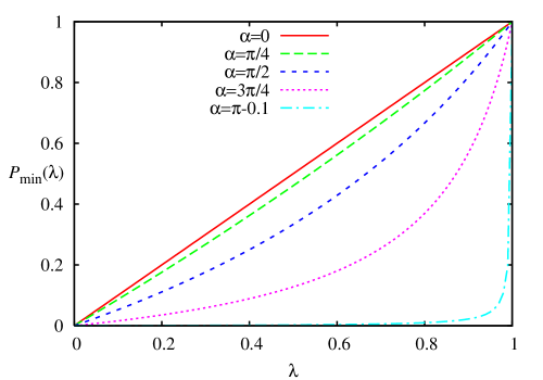
Figure 8: (Color online) Plots of $P_{\mathrm{min}}(\lambda)$ for $\alpha=0,\ \pi/4,\ \pi/2,\ 3\pi/4$, and $\pi-0.1$.

IV Summary

We have proposed a multi-phase matching for the Grover search algorithm, which is an extension of the new phase matching proposed in Ref. Li and Li (2007). The multi-phase matching is characterized by multiple Grover operations with two kinds of multi-phases $\alpha_{j}$ and $\beta_{j}$ $(j=1,\dots,k)$. We showed that if we match $\alpha_{j}$ and $\beta_{j}$ in accordance with the rule $\alpha_{j}=-\beta_{k-j+1}$ for a given $k$ we can obtain an optimal solution for $\alpha_{j}$, $\beta_{j}$ that gives a success probability curve such that it is almost constant and unity in a wide range of the fraction of marked states. As an example we presented an optimal solution obtained for $k=6$. The solution yields the desired success probability $P=1$ to within 0.2% for the fraction of the marked states greater than 0.1. This is significant in the sense that when the fraction of marked states is greater than 0.1, we can always with a high degree of confidence find a uniform superposition of the marked states by repeating the Grover operation just six times.

To clarify the mechanism of the multi-phase matching we studied in detail the one- and two-iteration cases. We showed that it is possible to obtain $P=1$ exactly for a particular fraction $\lambda$ by tuning the phases. This can be generalized to having $k$ values of $\lambda$ for which $P(\lambda)=1$ when we go to a $k$-iteration scheme.

One can obtain $P=1$ for a given very small $\lambda$ by using the original Grover algorithm or the phase-matched version of it. In this case usually a specified large number of iterations is required. Further study is needed to obtain an efficient algorithm for extremely small $\lambda$.

Appendix A Equivalence of two phase-matching schemes

Li and Li Li and Li (2007) claim to have generalized the Long phase-matching algorithm in order to produce a higher success probability. In actual fact the phase matching of Li and Li and that of Long et al. Long et al. (1999) result in the same success probability. We show that in the following.

Instead of Eqs. (1) and (2), Long et al. work with the operators

$$U=I-(1-e^{i\theta})\sum_{l=0}^{M-1}|t_{l}\rangle\langle t_{l}|$$ (45)

$$V=I-(1-e^{i\phi})|0^{\otimes n}\rangle\langle 0^{\otimes n}|.$$ (46)

These unitary transformations lead to the Grover operator (in the notation of this paper) $G(\theta,\phi)$, where

$$G=\begin{pmatrix}1-(1-e^{i\phi})(1-\lambda)&-(1-e^{i\phi})e^{i\theta}\sqrt{\lambda(1-\lambda)}\\ -(1-e^{i\phi})\sqrt{\lambda(1-\lambda)}&[1-(1-e^{i\phi})\lambda]e^{i\theta}\end{pmatrix}.$$ (47)

For one operation we calculate the final state

$$\begin{pmatrix}u\\ d\end{pmatrix}=G(\theta,\phi)\begin{pmatrix}\sqrt{1-\lambda}\\ \sqrt{\lambda}\end{pmatrix}$$ (48)

with

$$u=\sqrt{1-\lambda}[1-(1-e^{i\phi})(1-\lambda)-(1-e^{i\phi})e^{i\theta}\lambda].$$ (49)

Setting $u=0$ we obtain (in addition to $\lambda=1$) the solution

$$\phi=\theta,\ \ \ \lambda=\frac{1}{2}\frac{\cos\theta+1}{\sin^{2}\theta}.$$ (50)

Note that the signs of $\phi$ and $\theta$ are the same, unlike the opposite signs of the matched phases of Li and Li, i.e., $\beta=-\alpha$. In order that $0<\lambda\leq 1$ with this phase matching, $\theta$ varies from $\pi/3$ to $\pi$. For $P(\lambda)=1-|u|^{2}$, we obtain the expression of Eq. (12) with $\alpha$ replaced by $\theta$. Thus the impressive result by Li and Li of a single phase-matched Grover operation can also be obtained with the earlier-proposed operation of Long et al. However, the formulation of Li and Li results in $\mathrm{Im}\,u=0$ when $\beta=-\alpha$, whereas $\mathrm{Im}\,u\neq 0$ when $\phi=\theta$ for the operator of Long et al. It should be noted however that the remarkable single-operation result was first reported by Li and Li Li and Li (2007). Although the probabilities are the same the amplitudes are not, and Li and Li’s formulation gives a more straightforward derivation of the probabilities. (See Sec. IIA.) One can relate the two formulations by suggesting that instead of the operator acting on $(\sqrt{1-\lambda},\sqrt{\lambda})^{T}$ initially, in the case of Long et al. it operates on this state multiplied by a phase factor.

References

- (1)
- Grover (1996) L. K. Grover, in STOC ’96: Proceedings of the twenty-eighth annual ACM symposium on theory of computing (ACM, New York, NY, USA, 1996), pp. 212–219.
- Grover (1997a) L. K. Grover, Phys. Rev. Lett. 79, 325 (1997a).
- Grover (1997b) L. K. Grover, Phys. Rev. Lett. 79, 4709 (1997b).
- Grover (2001) L. K. Grover, Am. J. Phys. 69, 769 (2001).
- Grover (1998) L. K. Grover, Phys. Rev. Lett. 80, 4329 (1998).
- Long et al. (1999) G. L. Long, Y. S. Li, W. L. Zhang, and L. Niu, Phys. Lett. A 262, 27 (1999).
- Long et al. (2001) G. L. Long, H. Yan, Y. S. Li, C. C. Tu, J. X. Tao, H. M. Chen, M. L. Liu, X. Zhang, J. Luo, L. Xiao, et al., Phys. Lett. A 286, 121 (2001).
- Collins (2002) D. Collins, Phys. Rev. A 65, 052321 (2002).
- Tulsi et al. (2006) T. Tulsi, L. K. Grover, and A. Patel, Quant. Inform. Comp. 6, 483 (2006).
- Li and Li (2007) P. Li and S. Li, Phys. Lett. A 366, 42 (2007).
- Younes (2007) A. Younes, arXiv:quant-ph/0704.1585v2 (2007).
- Chi and Kim (1997) D. P. Chi and J. Kim, arXiv:quantum-ph/9708005v1 (1997).
- Høyer (2000) P. Høyer, Phys. Rev. A 62, 052304 (2000).
- Long (2001) G. L. Long, Phys. Rev. A 64, 022307 (2001).
- Grover (2005) L. K. Grover, Phys. Rev. Lett. 95, 150501 (2005).
- Pipes (1958) L. A. Pipes, Applied mathematics for engineers and physicists (Mc-Graw-Hill Book Company, Inc., Toronto, 1958), 2nd ed.
- Sprung et al. (1993) D. W. L. Sprung, H. Wu, and J. Martorell, Am. J. Phys. 61, 1118 (1993).