Selective Spin Injection Controlled by Electrical way in Ferromagnet/Quantum Dot/Semiconductor system

Abstract

Selective and large polarization of current injected into semiconductor (SC) is predicted in Ferromagnet (FM)/Quantum Dot (QD)/SC system by varying the gate voltage above the Kondo temperature. In addition, spin-dependent Kondo effect is also revealed below Kondo temperature. It is found that Kondo resonances for up spin state is suppressed with increasing of the polarization $P$ of the FM lead. While the down one is enhanced. The Kondo peak for up spin is disappear at $P=1$.

Effective spin injection into semiconductor is the central issue of spin-related semiconductor devices, such as the so-called spin-field-effect transistor (SFFT) proposed by Datta and Das datta which may be the original starting point of spintronics wolf . Spin-valve effect was predicted in it via controlling the gate voltage which controls the Rashba spin-orbit coupling parameter datta . Some experimental attempts were then performed to realize it but only small signal of spin injection had been observed. Schmidt et al. pointed out that the mismatch of conductance of FM and SC is the reason of the low efficiency of spin injection schmidt1 . However, Rashba proposed that a tunnel barrier can be inserted between the FM and SC to overcome this problem rashba . Soon, many experiments were then reported to confirm Rashba’s idea mtt ; tb . For example, hot electron current with a high spin polarization of about $98\%$ can be obtained mtt . On the other hand, other methods for spin filter or spin injection into semiconductor are also proposed, such as a FM tip of scanning tunnelling microscope is used to inject spin-polarized electrons into SC stm and a triple tunnel barrier diode is utilized as spin source to enhance the spin-filtering efficiency even to $99.9\%$ koga .

More recently, new attempts to realize the devices where the spin character of the injected and detected electrons could be voltage selected gruber slobodskyy , have been made. In these devices, the source-drain voltage-controlled spin filter effect is investigated in a magnetic resonant tunnelling diode structure in which the central spacer is made of dilute magnetic SC ZnMnSe. Zhu and Su zhu proposed a magnetic filed dependence spin filter effect based on ZnSe/ZnMnSe/ZnSe/ZnMnSe/ZnSe structure in which resonances of different spin components occur at different magnitude of magnetic field. These researches open new ways to controllable spin filter effect. However, these proposed structures are involved in dilute magnetic SC whose Curie temperature is known blow room temperature, preventing its further application in devices. In addition, for the difficulty of operating individual spin by external magnetic field, new attempt called all electrical devices is proposed in which the controlling are all via electrical ways.

In this letter, such a selective spin injection into semiconductor is predicted in Ferromagnet (FM)/Quantum Dot (QD)/SC system by varying the gate voltage which controls the states of the QD. A FM layer holding high Curie temperature (above room temperature) is used as a spin source and polarized electrons flowing out of it tunnel through a vertical QD (VQD) vqd into SC. Between the two tunnel barrier a quantum well is defined as a QD with strong Coulomb interaction. The energy levels of QD can be tunned by a gate voltage $V_{g}$. It is found the polarization of current is large and can be controlled by tunning $V_{g}$ from negative to positive (from down-spin filtering to up-spin filtering) because of the mixed roles of Coulomb interaction and the splitting of spin subbands of FM. It is worth pointing out that the splitting of energy levels of QD for different spins are large and corresponds to the Curie temperature order. This large splitting guarantees the well-defined separation of polarized current with different spins and the spin filter effect.

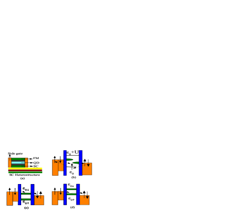
Figure 1: (color online). (a) The model configuration. (b) The formation of spin-dependent Kondo resonances for spin-polarized lead. (c) and (d) The developed spin-dependent resonant tunnelling. $\varepsilon_{0\uparrow}$ and $\varepsilon_{0\downarrow}$ have finite width for the imaginary of selfenergy.

The Hamiltonian is $H=H_{leads}+H_{dot}+H_{T}$, $H_{leads}=\sum_{k\sigma}\varepsilon_{k\sigma}^{L}a_{k\sigma}^{\dagger}a_{k\sigma}+\sum_{q\sigma}\varepsilon_{qR}b_{q\sigma}^{\dagger}b_{q\sigma}$, $H_{dot}=\sum_{\sigma}\epsilon_{0}d_{\sigma}^{\dagger}d_{\sigma}+Un_{d\uparrow}n_{d\downarrow}$, $H_{T}=\sum_{k\sigma}[t_{kL}^{\sigma}a_{k\sigma}^{\dagger}d_{\sigma}+h.c.]+\sum_{q\sigma}[t_{qR}^{\sigma}b_{q\sigma}^{\dagger}d_{\sigma}+h.c.]$, where $\varepsilon_{k\sigma}^{L}=\varepsilon_{kL}-\mu_{L}-\sigma M$, $M=g\mu_{B}h/2$, $g$ is Landé factor, $\mu_{B}$ is Bohr magneton, $h$ is the molecular field, $\varepsilon_{kL}$ is the single-particle dispersion of the left FM, $\mu_{L(R)}$ is the Fermi level of the left (right) lead, $n_{d\sigma}=d_{\sigma}^{\dagger}d_{\sigma}$, $\varepsilon_{qR}=\hbar^{2}q^{2}/2m^{\ast}$, $m^{\ast}$ is effective mass of electrons in the right lead, $t_{kL(qR)}^{\sigma}$ denotes the tunnelling amplitude through the left (right) barrier.

Then following the standard equation of motion method, and assuming that higher-order spin-correlations in the leads can be neglected assum , the Green function $\langle\langle d_{\sigma}|d_{\sigma^{\prime}}^{\dagger}\rangle\rangle^{r}$ can be obtained

$$\langle\langle d_{\sigma}|d_{\sigma^{\prime}}^{\dagger}\rangle\rangle^{r}=\frac{(\varepsilon-\widetilde{\epsilon}_{\sigma}+U\left\langle n_{\overline{\sigma}}\right\rangle)\delta_{\sigma\sigma^{\prime}}-U\left\langle d_{\overline{\sigma}}^{\dagger}d_{\sigma}\right\rangle\delta_{\overline{\sigma}\sigma^{\prime}}}{(\varepsilon-\widetilde{\epsilon}_{\sigma})(\varepsilon-\epsilon_{0}-\Sigma_{\sigma}^{0})+U\Sigma_{\overline{\sigma}}^{1}},$$ (1)

where $\widetilde{\epsilon}_{\sigma}=\epsilon_{0}+U+\Sigma_{\sigma}^{0}+\Sigma_{\overline{\sigma}}^{3}$, $\Sigma_{\sigma}^{L(R)0}=\int\frac{d\varepsilon^{\prime}}{2\pi}\frac{\Gamma_{\sigma}^{L(R)}(\varepsilon^{\prime})}{\varepsilon-\varepsilon^{\prime}+i\eta}$, $\Sigma_{\overline{\sigma}}^{2}=\Sigma_{\overline{\sigma}}^{3}-\Sigma_{\overline{\sigma}}^{1}$, $\Sigma_{\overline{\sigma}}^{L(R)\lambda}=\int\frac{d\varepsilon^{\prime}}{2\pi}\Gamma_{\overline{\sigma}}^{L(R)}(\varepsilon^{\prime})B\digamma(\varepsilon^{\prime})$, ($B=1$, $\lambda=3$; $B=f_{L(R)}$, $\lambda=1$), where $\digamma(\varepsilon^{\prime})=\frac{1}{\varepsilon-(2\epsilon_{0}+U)+\varepsilon^{\prime}+i\eta}+\frac{1}{\varepsilon-\varepsilon^{\prime}+i\eta}$, $\Gamma_{\sigma}^{L}(\varepsilon^{\prime})=2\pi\mathbf{\rho}_{L}(\varepsilon^{\prime}+\sigma M)\left|t_{L}^{\sigma}(\varepsilon^{\prime})\right|^{2}$, $\Gamma_{\uparrow}^{R}=\Gamma_{\downarrow}^{R}=\Gamma^{R}(\varepsilon^{\prime})=2\pi\rho_{R}(\varepsilon^{\prime})\left|t_{R}(\varepsilon^{\prime})\right|^{2}$, $\mathbf{\rho}_{L(R)}$ is density of state (DOS) of the left (right) lead and $\Sigma_{\sigma}^{\gamma}=\Sigma_{\sigma}^{L\gamma}+\Sigma_{\sigma}^{R\gamma}$ ($\gamma=1,2,3$). The retard selfenergy can be derived from Dyson equation $\mathbf{\Sigma}^{r}=(\mathbf{g}^{r})^{-1}-(\mathbf{G}^{r})^{-1}$, where $\mathbf{g}^{r}$ is the retard GF of QD without coupling to the leads but with Coulomb interaction. To get $\left\langle n_{\overline{\sigma}}\right\rangle$, the selfconsistent calculation must be preformed selfconsist . And this procedure needs lesser Green function which is subject to the Keldysh formula $G^{<}=G^{r}\Sigma^{<}G^{a}$. The lesser self-energy is taken the form as $\Sigma^{<}=\frac{1}{2}[\Sigma_{0}^{<}(\Sigma_{0}^{r}-\Sigma_{0}^{a})^{-1}(\Sigma^{r}-\Sigma^{a})+(\Sigma^{r}-\Sigma^{a})(\Sigma_{0}^{r}-\Sigma_{0}^{a})^{-1}\Sigma_{0}^{<}]$ self , where $\Sigma_{0}^{r(a,<)}$ are the selfenergies of the noninteracting system while $\Sigma^{r(a,<)}$ are selfenergies with full interaction. In fact, one method without solving $G^{<}$ and only with calculating the integral $\int d\varepsilon G^{<}(\varepsilon)$ exactly has been developed to round the calculation of the lesser Green function sun1 . However, the approximation used here to derive the lesser Green function can give a qualitatively correct results. We shall mention that $\left\langle d_{\overline{\sigma}}^{\dagger}d_{\sigma}\right\rangle$ in principle tends to zero without spin flip scattering. We keep it here to avoid any uncertainty which might be caused by self-consistent calculation procedure and its value can be given by the self-consistent calculation.

No losing generality, we shall do numerical calculations in the limit $U\rightarrow\infty$. We use $\Gamma_{0}^{L}$ as the unit of energy, which is defined in terms of the unpolarized parabolic energy bands parameters, and $J_{0}=e\Gamma_{0}^{L}/\hbar$ as current unit. We set $P=\frac{\rho_{\uparrow}^{L}-\rho_{\downarrow}^{L}}{\rho_{\uparrow}^{L}+\rho_{\downarrow}^{L}}$, $t_{qR(kL)}^{\uparrow}=t_{qR(kL)}^{\downarrow}=t_{R(L)}$, then $\chi_{\uparrow}=\Gamma_{\uparrow}^{L}/\Gamma_{0}^{L}=(\frac{2}{1+\chi^{2}})^{\frac{1}{2}}$, $\chi_{\downarrow}=\Gamma_{\downarrow}^{L}/\Gamma_{0}^{L}=\chi\chi_{\uparrow}$, where $\chi=\frac{1-P}{1+P}$. Let $\chi_{R}=\Gamma^{R}/\Gamma_{0}^{L}=\alpha$. The left lead is FM and the right lead is SC, and the $\Gamma^{L(R)}$ is in proportion to the DOS of the left (right) lead. So we may estimate the $\alpha$ will be between $10^{-4}\rightarrow 10^{-3}$ (for the right SC lead, we use 3D DOS rather than using 2D DOS to avoid the complexity). But if the tunnelling matrix $t_{(L)R}$ can be tuned to be different, the parameter $\alpha$ may be tuned till $1$ (this case is considered in Fig. 4). To get the retard Green function, selfenergy $\Sigma_{\sigma}^{1}$ will be calculated analytically as s1

$$\Sigma_{\sigma}^{L1}(\Sigma^{R1})=\frac{\Gamma_{\sigma}^{L}(\Gamma^{R})}{2\pi}\{\frac{1}{2}\ln\frac{\varepsilon_{1}\varepsilon_{2}}{(2\pi iT)^{2}}-\psi(z)-\frac{i}{2}\pi\},$$ (2)

where $\varepsilon_{1}=\varepsilon-\mu_{L(R)}-D$, $\varepsilon_{2}=\varepsilon-\mu_{L(R)}+D$, $z=\frac{1}{2}+\frac{\varepsilon-\mu_{L(R)}}{2\pi iT}$, $D$ is the half bandwidth, and we set it as 1500 in this letter, $T$ is temperature.

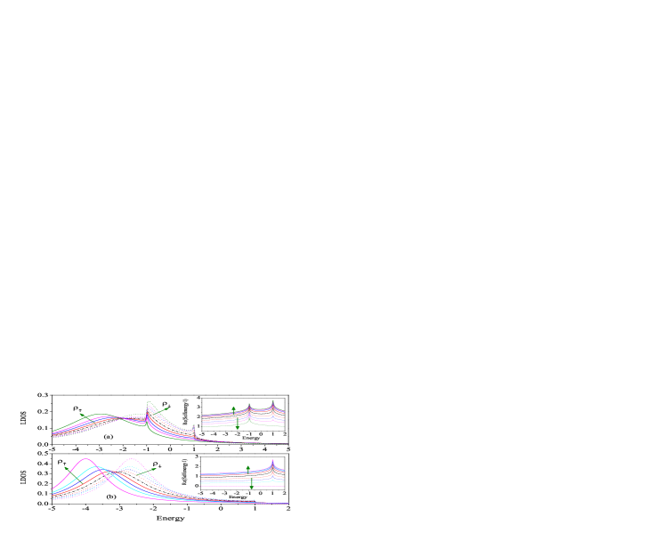
Figure 2: (color online). In the four graphs, dash-dot lines are generated at $P=0$, and solid (dot) lines for $\rho_{\uparrow}$ ($\rho_{\downarrow}$) or $\Re\Sigma_{\uparrow}^{1}$ ($\Re\Sigma_{\downarrow}^{1}$ ). Along the directions of the arrows, the lines are sequently corresponding to $P=0.2,$ $0.4,$ $0.6,$ and $1$. LDOS vs. energy in (a) and (b), $\Re\Sigma_{\sigma}^{1}$ in insets. $\alpha=1$ in (a) and its inset; $\alpha=0.001$ in (b) and its inset. The other parameters are $T=0.01$, $\varepsilon_{0}=-4$, and $V=2$ ($\varepsilon_{0}$ and $V$ are the same in all figures).

Local density of state (LDOS) ldos $\rho_{\sigma}(\varepsilon)$ and $\Re\Sigma_{\sigma}^{1}$ in QD vs. energy for different polarization $P$ are shown in Fig. 2. It can be found that $\rho_{\uparrow}(\varepsilon)$ and $\rho_{\downarrow}(\varepsilon)$ are split because of FM lead. The main peaks of LDOS exist at the resonant energy $\varepsilon=\varepsilon_{0\sigma}$, where $\varepsilon_{0\sigma}=\varepsilon_{0}+\Re\Sigma_{\overline{\sigma}}^{1}$ indicates that the original spin-independent energy level is modified as spin-dependent energy levels because of Coulomb interaction on QD and the polarization $P$. $\Re\Sigma_{\overline{\sigma}}^{1}$ is proportional to the tunnelling rate $\Gamma_{\overline{\sigma}}^{L}$ which depends on $P$. $\Re\Sigma_{\uparrow}^{1}$ ($\Re\Sigma_{\downarrow}^{1}$) increases (decreases) with $P$ and show two resonances at $-V/2$ and $V/2$ except for $\Re\Sigma_{\downarrow}^{1}$ at $P=1$ as shown in the inset of Fig. (2a). This increasing (decreasing) gives rise to the shift of the main peak of $\rho_{\uparrow}(\varepsilon)$ ($\rho_{\downarrow}(\varepsilon)$) towards to the lower (higher) energy.

Kondo resonances (KRs) of $\rho_{\uparrow}(\varepsilon)$ and $\rho_{\downarrow}(\varepsilon)$ existing about at $\mu_{L}=V/2$ and $\mu_{R}=-V/2$ shown in Fig. (2a) are consequences of nonequilibrium effect meir . i) With increasing $P$, the magnitude of KRs for down (up) spin component is higher (lower). While the peak of $\Re\Sigma_{\downarrow}^{1}$ disappears at $V/2$ and $P=1$ in the inset of Fig. (2a), the corresponding KR of $\rho_{\uparrow}(\varepsilon)$ disappears also. But the other KRs of $\rho_{\uparrow}(\varepsilon)$ bounded at $-V/2$ remain. The reason is there are no itinerant spin-down electrons in the FM layer for formation of spin singlet with the electrons on QD now. ii) The positions of spin-up KRs move to lower energy and the spin-down ones move to the opposite direction. Spin-dependent Kondo effect was firstly investigated in FM-QD-FM system in Ref. sergueev . Then further theoretical martinek and experimental pas investigations are evaluated to show the splitting of the Kondo resonances. However it has no influences on the spin filter effect which is mainly investigated in a temperature scale much above the Kondo temperature.

Higher order cotunneling processes sasakl depicted in Fig. (1b) account for the formation of these KRs. Initially, an up-spin electron occupies the QD, it can jump to the left (right) lead at a time scale $\hbar/(\mu_{L(R)}-\varepsilon_{0})$. Almost at the same time, a down-spin electron of the right (left) lead can jump into the QD. Then the final state is a spin-flip state. A large number of coherent superpositions of these events will give rise to KRs at Fermi levels. The conduction electrons tend to screen the nonzero spin on QD such that a many-body spin singlet state forms. This process can transfer charges from one lead to the other and then the KR may enhance the conductance or current ng . Another contributing process is that a spin occupying the QD jumps into one lead and almost at the same time an opposite spin in the same lead tunnels into QD, which can be clearly seen from the Eq. (239) in Ref. platero in which the Hamiltonian consisting the QD and leads is transformed into a Hamiltonian similar to the conventional Kondo Hamiltonian via Schrieffer-Wolff transformation sw . There $J_{LL}$ and $J_{RR}$ describe the coupling of the local spin on QD and the spins of itinerant electrons in the left or right leads respectively. This process doesn’t transfer charge from one lead to the other.

When $\alpha$ is very small (for example $\alpha=0.001$ in Fig. (2b) and its inset), $\Sigma^{R1}$ contributes little to $\Re\Sigma_{\sigma}^{1}$. The channel of formation KRs between QD and the right lead is suppressed. So in Fig. (2b) and its inset, the peaks about at $-V/2$ all disappear, but the KRs about at $V/2$ are still present. The spin-splitting of $\rho_{\uparrow}(\varepsilon)$ and $\rho_{\downarrow}(\varepsilon)$ remains, giving rise to the spin filter effect described in the following.

To investigate the spin-filter effect, we shall calculate the current through this structure. By using the nonequilibrium Green function technique negf , the steady current with up (down) spin in unit $J_{0}$ is

$$J_{\uparrow(\downarrow)}/J_{0}=\Delta_{1(2)}\int d\varepsilon[f_{L}(\varepsilon)-f_{R}(\varepsilon)]\rho_{d\uparrow(d\downarrow)}(\varepsilon),$$ (3)

where $\Delta_{1}=\frac{\chi_{\uparrow}\alpha}{\chi_{\uparrow}+\alpha}$ and $\Delta_{2}=\frac{\chi_{\downarrow}\alpha}{\chi_{\downarrow}+\alpha}$. When a gate voltage is applied, we set new energy level on QD is $\varepsilon_{0}^{\prime}=\varepsilon_{0}+V_{g}$. The spin polarization of current is defined as $P_{out}=\frac{J_{\uparrow}-J_{\downarrow}}{J_{\uparrow}+J_{\downarrow}}$, which is not the polarization of the DOS of the left lead. When $P=0$, i.e. the injector is spin independent, $\Delta_{1}=\Delta_{2}$ and $P_{out}=0$. When $P=1$, i.e. the injector is fully polarized (for example half-metal material), $\Delta_{2}=0$ and $P_{out}=1$. When $0<P<1,$ at the limit $\alpha\rightarrow 0$, $\Delta_{1}\approx\Delta_{2}\approx\alpha$, then $P_{out}$ just depends on the difference of the LDOS of QD for different spins.

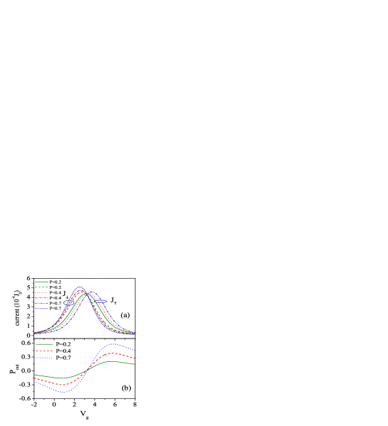
Figure 3: (color online). The $V_{g}$ dependence of current in (a) and $P_{out}$ in (b). $\alpha=0.001$ and $T=0.5$.

Quite usually, devices are operated in room temperature which is much higher than Kondo temperature, and KRs disappear. The $V_{g}$ dependence of $J_{\uparrow}$ and $J_{\downarrow}$ are presented in Fig. (3a). It is noted that currents have resonant peaks which are split under nonzero $P$ because of $\varepsilon_{0\uparrow}\neq\varepsilon_{0\downarrow}$. And the splitting becomes larger with increasing $P$. It can be understood that when $\varepsilon_{0\uparrow(\downarrow)}$ is in the energy range $[-V/2,V/2]$ as shown in Fig. (1c) and (1d), resonant tunnelling occurs and a resonant peak of $J_{\uparrow(\downarrow)}$ present. When $\varepsilon_{0\uparrow(\downarrow)}$ is out of this range, current is suppressed. We call this range as resonant window (RW). As $\varepsilon_{0\downarrow}>\varepsilon_{0\uparrow}$, $\varepsilon_{0\downarrow}$ first enters into the RW with increasing $V_{g}$ as shown in Fig. (1c), now $J_{\downarrow}$ is on-resonant and $J_{\uparrow}$ is off-resonant. Increasing $V_{g}$ further, $\varepsilon_{0\uparrow}$ enters into the RW as shown in Fig. (1d), and the case is opposite to the former. When $V_{g}>V_{g0}$ (we set $J_{\uparrow}=J_{\downarrow}$ at $V_{g0}$), $P_{out}>0$; $P_{out}$ first increases and then decreases with $V_{g}$. When $V_{g}<V_{g0}$, $P_{out}<0$; $P_{out}$ also first increases and then decreases with $V_{g}$ as shown in Fig. (3b). Even $\alpha$ is very small, there is still a large $P_{out}$. For example, when $P=0.7$, the peak magnitude of $P_{out}$ is 0.58 ($V_{g}=5.83$), and the peak magnitude is enhanced by increasing $P$. $P_{out}$ varies from negative to positive with increasing gate voltage, which means the spin filter effect can be controlled by tuning the gate voltage.

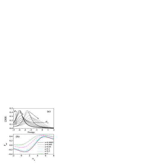
Figure 4: (color online). LDOS vs. energy in (a) and $V_{g}$ dependence of $P_{out}$ in (b) for different $\alpha$. In (a) along the directions of arrows the lines correspond to $\alpha=0.001,$ $0.05$, $0.1$, $0.3$, $0.5$, $0.7$, and $1$. The other parameters are $P=0.4,$ $T=0.5$.

LDOS vs. energy in Fig. (4a) and $V_{g}$ dependence of $P_{out}$ in Fig. (4b) for different $\alpha$. $\rho_{\uparrow}$ and $\rho_{\downarrow}$ become lower and fatter with increasing $\alpha$. It means the local electrons on QD tend to be nonlocal and tunnel to the right lead. And the main peaks are shifted towards the right direction shown in Fig. (4a). It is found that negative $P_{out}$ is reduced and even becomes positive with increasing $\alpha$ in Fig. (4b). On the other hand, the positive $P_{out}$ will be enhanced with $\alpha$. For example, when $\alpha=1$, there is no negative $P_{out}$. But the maximum of $P_{out}$ is enhanced to give 0.464 for $\alpha=1$ and $P=0.4$.

The effect predicted here is the consequence of well-defined spin-dependent energy levels of QD. So spin relaxation in QD may reduce the effect and we may estimate its order. For comparison, in Ref. gruber , spin relaxation time (SRT) is shorter in ZnMnSe layer because of the spin-dependent scatterings in it. However, SRT is much longer in our case. Firstly, it is because the QD is formed in the nonmagnetic semiconductor quantum well, spin-dependent scatterings are sparse. Secondly, the zero dimensionality of electron states in QDs leads to a significant suppression of the most effective 2D spin-flip mechanisms kha , and the electron spin states in QDs are expected to be very stable. Recent electrical transport measurements of relaxation between spin triplet and singlet states confined in a VQD give relaxation time $>200\mu s$ at $T\leq 0.5$ K fuj . Finally, we estimate the transit time. For a typical value $\Gamma=150$ $\mu V$ sasakl ($\Gamma$ can be changed by changing the barrier thickness gueret ), the estimated transit time is about $5$ $ps$. So it seems reasonable to assume that the spin relaxation on QD has little effect in this model.

In Ref. gruber , the spin dependent energy levels are induced by Zeeman splitting under an external magnetic field in magnetic semiconductor ZnMnSe quantum well. While in this letter the tunnelling rates for up and down spins are split because of the splitting of DOS of FM. This splitting likes an effective magnetic field (EMF) but much stronger than conventional magnetic field, even reach $50\sim 70$ T ralph , leading to the well defined spin-dependent energy levels on QD. Further an upper limit on the local magnetic field (LMF) which is generated by FM lead in QD is estimated to be 0.6 T for Ni hanson . It seems reasonable to neglect this LMF.

In summary, selective and large polarization of current injected into semiconductor is predicted in Ferromagnet /Quantum Dot /semiconductor system by varying the gate voltage above the Kondo temperature. A FM layer is used as a spin source and electrons tunnel through a QD into SC. Spin-dependent Kondo effect is revealed below Kondo temperature. KRs for up spin state is suppressed with $P$. While the down one is enhanced. The KR for up spin is disappear at $P=1$. With increasing the gate voltage, the polarization of current varies from negative to positive, which means spin filter effect can be controlled by gate voltage. A large efficient spin injection can be obtained.

This work was supported by the Natural Science Foundation of China (Grant Nos. 10574076, 10447118), and by the Program of Basic Research Development of China (Grant No. 2006CB921500).

References

- (1) S. Datta and B. Das, Appl. Phys. Lett. 56, 665 (1990).
- (2) S. A. Wolf et al., Science 294, 1488 (2001).
- (3) G. Schmidt et al., Phys. Rev. B 62, R16267 (2000).
- (4) E. I. Rashba, Phys. Rev. B 62, R4790 (2000).
- (5) X. Jiang et al., Phys. Rev. Lett. 90, 256603 (2003); S. van Dijken et al., ibid. 90, 197203 (2003); Phys. Rev. B 66, 094417 (2002); Appl. Phys. Lett. 80, 3364 (2002).
- (6) T. Manago and H. Akinaga, Appl. Phys. Lett. 81, 694 (2002); V. F. Motsnyi et al., ibid. 81, 265 (2002); A. T. Hanbicki et al., ibid. 80, 1240 (2002); 82, 4092 (2003); S. Kreuzer et al., ibid. 80, 4582 (2002); Y. Q. Jia et al., IEEE Transactions on Magnetics, 32, 4707 (1996); H. J. Zhu et al., Phys. Rev. Lett. 87, 016601 (2001); A. F. Isakovic et al., J. Appl. Phys. 91, 7261 (2002).
- (7) S. F. Alvarado and P. Renaud, Phys. Rev. Lett. 68, 1387 (1992).
- (8) T. Koga et al., Phys. Rev. Lett. 88, 126601 (2002).
- (9) Th. Gruber, et al., Appl. Phys. Lett. 78, 1101 (2001).
- (10) A. Slobodskyy et al., Phys. Rev. Lett. 90, 246601 (2003).
- (11) Zhen-Gang Zhu and Gang Su, Phys. Rev. B 70, 193310 (2004).
- (12) S. Tarucha et al., Phys. Rev. Lett. 77, 3613 (1996); ibid. 84, 2485 (2000); I. I. Yakimenko et al., Phys. Rev. B 63, 165309 (2001); M. Rontani et al., ibid 69, 085327 (2004); K. Ono et al., Science 297, 1313 (2002).
- (13) It means that correlation function which invovle unlike spin-indices, invovle different operators of the left and the right leads or both creat operators (annihlation operators) equal to zero, and factorize the correlation functions with like spin .
- (14) , , where means lesser GF derived from the returded GF by using Keldysh formula. Given these two initial values, then substitute them into the retard Green function and Keldysh formula to get them for the second time. This procedure continues to give a constant and . The retard Green function and lesser Green function can be obtained.
- (15) T. -K. Ng, Phys. Rev. Lett. 76, 487 (1996); Qing-feng Sun et al., ibid. 87, 176601 (2001).
- (16) Qing Feng Sun, and Hong Guo, Phys. Rev. B 66, 155308 (2002).
- (17) P. E. Bloomfield and D. R. Hamann, Phys. Rev. 164, 856 (1967).
- (18) The local density of states (LDOS) is defined as .
- (19) Y. Meir et al., Phys. Rev. Lett. 70, 2601 (1993); N. S. Wingreen and Y. Meir, Phys. Rev. B. 49, 11040 (1994).
- (20) N. Sergueev, Qing-feng Sun, Hong Guo, B. G. Wang, and Jian Wang, Phys. Rev. B 65, 165303 (2002).
- (21) J. Martinek, et al., Phys. Rev. Lett. 91, 127203 (2003).
- (22) A. N. Pasupathy, et al., Science 306, 86 (2004).
- (23) S. Sasakl et al., Nature 405, 764 (2000).
- (24) T. K. Ng and P. A. Lee, Phys. Rev. Lett. 61, 1768 (1988).
- (25) G. Platero and R. Aguado, Phys. Rep. 395, 1 (2004).
- (26) J. R. Schrieffer and P. A. Wolff, Phys. Rev. 149, 491 (1966).
- (27) A. P. Jauho et al., Phys. Rev. B 50, 5528 (1994); H. Haug and A. -P. Jauho, Quantum Kinetics in Transport and Optics of Semiconductors (Springer-Verlag, Berlin, 1998).
- (28) A. V. Khaetskii and Y. N. Nazarov, Phys. Rev. B 61, 12639 (2000).
- (29) T. Fujisawa, et al., Nature (London) 419, 278 (2002).
- (30) P. Guéret, et al., J. Appl. Phys. 66, 278 (1989).
- (31) A. N. Pasupathy, et al., Science 306, 86 (2004).
- (32) R. Hanson, et al., Phys. Rev. Lett. 91, 196802 (2003).