Evidence for collisional depolarization of the Ba ii ${\lambda}4554$ line in the low chromosphere

Abstract

Context. Rigorous modeling of the Ba ii ${\lambda}4554$ formation is potentially interesting since this strongly polarized line forms in the solar chromosphere where the magnetic field is rather poorly known.

Aims. To investigate the role of isotropic collisions with neutral hydrogen in the formation of the polarized Ba ii ${\lambda}4554$ line and, thus, in the determination of the magnetic field.

Methods. Multipole relaxation and transfer rates of the $d$ and $p$-states of Ba ii by isotropic collisions with neutral hydrogen are calculated. We consider a plane parallel layer of Ba ii situated at the low chromosphere and anisotropically illuminated from below which produces linear polarization in the ${\lambda}4554$ line by scattering processes. To compute that polarization, we solve the statistical equilibrium equations for Ba ii levels including collisions, radiation and magnetic field effects.

Results. Variation laws of the relaxation and transfer rates with hydrogen number density $n_{\textrm{\scriptsize H}}$ and temperature are deduced. The polarization of the ${\lambda}4554$ line is clearly affected due to isotropic collisions with neutral hydrogen although the collisional depolarization of its upper level ${}^{2}P_{3/2}$ is negligible. This is because the alignment of the metastable levels ${}^{2}D_{3/2}$ and ${}^{2}D_{5/2}$ of the Ba ii are vulnerable to collisions. At the height of formation of the ${\lambda}4554$ line where $n_{\textrm{\scriptsize H}}\sim 2\times 10^{14}$ cm^-3, we find that the neglecting of the collisions induces inaccuracy of $\sim$ 25% on the calculation of the polarization and $\sim$ 35 % inaccuracy on microturbulent magnetic field determination.

Conclusions. The polarization of the ${\lambda}4554$ line decreases due to collisions with hydrogen atoms. In addition, during scattering processes collisions could change the frequency of the Ba ii photons. To quantitatively study this line, one should confront the problem of development of general theory treating partial redistribution of frequencies and including transfer and relaxation rates by collisions for a multilevel atom with hyperfine structure.

1 Introduction

Depolarization due to the Hanle effect can be used to retrieve information on solar magnetic fields (e.g. Trujillo Bueno 2001). This magnetic depolarization is usually mixed with a collisional depolarization. To quantitatively use the Hanle effect as a technique of investigation of solar magnetic fields, one needs to know the collisional rates. In addition, one should include properly both the collisional depolarizing and transfer rates in the line formation modeling. For instance, Derouich et al. (2007) found that the effect of the collisions, in typical solar conditions of temperature and hydrogen density, is particularly important for the very important Ti i ${\lambda}4536$ line– a collisional depolarization of more than 25 % is obtained. In fact, at a first glance, because the inverse lifetime of the upper level is larger than the value of the elastic depolarizing rate $D^{2}$, one might think (wrongly) that the effect of the collisions is negligible for the Ti i ${\lambda}4536$ line. Collisional depolarization of this line is mainly due to transfer rates which are generally neglected (see Eq. 14 of Derouich et al. 2007).

Since their ionization potential is rather low, most Barium atoms are ionized throughout the low chromosphere (Tandberg-Hanssen & Smythe 1970). The core of the Ba ii ${\lambda}4554$ line is formed at about 800 km above the photosphere (e.g. Uitenbroek & Bruls 1992). The wings are formed in deeper layers of the photosphere. Recently, a renewed interest in the measurement and the physical interpretation of the linear polarization of the Ba ii ${\lambda}4554$ line have emerged (e.g. Malherbe et al., 2007; Belluzzi et al. 2007; Lopez Ariste et al. 2008). It has been shown that during the formation of this line the hyperfine structure and the partial redistribution of the frequencies effects are very important. In this work, we investigate fully the importance of isotropic collisions with neutral hydrogen in its modeling (Sects. 2 and 3). Sect. 4 is dedicated to the calculation of the impact of neglecting collisional effects on the magnetic field determination. Our concluding remarks are given in Sect. 5.

2 Modeling of the creation of the polarization in the Ba ii levels

Let us consider a plane-parallel layer in the low chromosphere ($\sim$ 800 km above the photosphere) formed by Ba ii ions and illuminated anisotropically by the photospheric continuum radiation field. In a weakly polarizing medium like the solar atmosphere one can safely neglect the contribution of polarization to the excitation of Ba ii ions. Assuming that the incident radiation has cylindrical symmetry around the local solar vertical through the scattering center, only the multipole orders $k$ = 0 (mean intensity $J^{0}_{0}$) and $k$ = 2 (radiation tensor $J^{2}_{0}$ associated to the anisotropy) are needed to fully describe the incident radiation. For each wavelength, the value of the anisotropy factor ($w=\sqrt{2}J^{2}_{0}/J^{0}_{0}$) and of the number of photons per mode ($\bar{n}=J^{0}_{0}(c^{2}/2h\nu^{3})$) are obtained from Fig. 2 of Manso Sainz & Landi Degl’Innocenti (2002). In particular, for the Ba ii ${\lambda}4554$ line, we obtain $w=0.16$ and $\bar{n}=2.59\times 10^{-3}$ which are similar to the values calculated by Belluzzi et al. (2007). We verified that a reasonable modification of $w$ and $\bar{n}$ (i.e. by around 10%) do not affect the results of the present work. Obviously, a realistic simulation of the line formation conditions requires a careful consideration of the transfer of radiation in a medium that is not optically thin. This problem is out of the scope of this paper. The formulae we use to compute the linear polarization for the case of a tangential observation in a plane-parallel atmosphere is presented, for example, in Sect. 2 of Derouich et al. (2007).

A simplified atomic model approximation (Fig. 1) can reduce considerably the numerical and theoretical calculations especially if the transfer of radiation effects are considered. However, the hypothesis of neglecting metastable $d$-sates in the Ba ii ${\lambda}4554$ line modeling is highly questionable. We calculate the polarization $p=Q/I$ using the simplified atomic model (see Fig. 1) and the 5 levels-5 lines model (see Fig. 2) which accounts for the metastable $d$-levels. We find that the simplified model overestimates the polarization degree of the Ba ii ${\lambda}4554$:

$$\frac{{(p)}_{\textrm{5 levels-5 lines model}}}{{(p)}_{\textrm{simplified model}}}\simeq 0.7$$ (1)

Thus, a more realistic diagnostic of the polarization of this line should be performed in the framework of 5 levels-5 lines model. In the description of the Ba ii, we neglect the contribution of the hyperfine structure. There are no additional conceptual difficulties for including the contribution of the hyperfine relaxation and polarization transfer rates by isotropic collision. Our main conclusions concerning the evidence for collisional depolarization of the Ba ii ${\lambda}4554$ line remain unchanged.

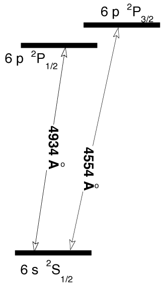
Figure 1: Partial Grotrian diagram of Ba ii showing the levels and the spectral wavelengths taken into account in the case of the simplified model. Note that the level spacings are not to scale.

3 Contribution of collisions in the framework of the 5 levels-5 lines model

3.1 Definitions of the depolarization, relaxation, and polarization transfer rates and statistical equilibrium equations

The collisional evolution of the density matrix components $\rho_{q}^{k}(J)$ is due to the gain-terms denoted as polarization transfer rates and to the loss-terms denoted as relaxation rates. The polarization transfer rates, denoted by $C_{I}(k\;J\leftarrow k\;J^{\prime},\;T)$ if $E_{J}>E_{J}^{\prime}$ and $C_{S}(k\;J\leftarrow k\;J^{\prime})$ if $E_{J}<E_{J}^{\prime}$, are due to inelastic and super-elastic collisions respectively. $E_{J}$ being the energy of the $J$-level. The left arrow ($\leftarrow$) is used because these rates represent gain-terms in the statistical equilibrium equations (SEE) describing the evolution of the $J$-level.

The relaxation rates are the sum of the term $D^{k}(J,\;T)$ exclusively responsible for the depolarization of the level $(J)$ and the terms $C_{I}(k=0\;J\to k=0\;J^{\prime},\;T)$ ($E_{J}<E_{J}^{\prime}$) and $C_{S}(k=0\;J\to k=0\;J^{\prime},\;T)$ ($E_{J}>E_{J}^{\prime}$) corresponding to the population transfer between the levels $J$ and $J^{\prime}$. We notice that, in principle, the denotations “inelastic” and “superelastic” are used for transitions between different electronic sates. Within the same spectral term (inside a given electronic state), collisions are called “elastic” even these involving transitions between two different $J$-levels. However, we adopt the denotations $C_{S}$ and $C_{I}$ since they are usually used in astrophysics. We denote by $R^{k}(J,\;T)$ the relaxation rates of rank $k$ given by:

$$R^{k}(J,\;T)=D^{k}(J,\;T)+R^{0}(J,\;T)=D^{k}(J,\;T) + \sum_{J_{l}}\sqrt{\frac{2J_{l}+1}{2J+1}}\;C_{S}(k=0\;J\to k=0\;J_{l},\;T)$$

$$+\sum_{J_{u}}\sqrt{\frac{2J_{u}+1}{2J+1}}\;C_{I}(k=0\;J\to k=0\;J_{u},\;T)$$

The overall population of the level $J$ is not affected by purely elastic collisions, $D^{0}(J,\;T)$=0. The SEE are:

$$\big{[}\frac{d}{dt}\;\rho_{q}^{k}(J)\big{]}_{\rm coll} = -R^{(k)}(J,\;T)\;\rho_{q}^{k}(J)+\sum_{J_{l}}C_{I}(k\;J\leftarrow k\;J_{l},\;T)\;\rho_{q}^{k}(J_{l})$$ (3)

$$+\sum_{J_{u}}C_{S}(k\;J\leftarrow k\;J_{u},\;T)\;\rho_{q}^{k}(J_{u})$$

Despite $-k\;\leq\;q\;\leq\;k$, due to the isotropy of the collisions with neutral hydrogen, the relaxation and polarization transfer rates are calculated only for $q=0$ since they are $q$-independent. The effect of the isotropic collisions is the same for density matrix elements with $q=0$ and for off-diagonal ones corresponding to coherences where $q\neq 0$.

In the standard case where polarization phenomena are neglected, the SEE can be obtained from Eq. (3) simply by retaining the terms with $k=q=0$:

$$\big{[}\frac{d}{dt}\;\rho_{0}^{0}(J)\big{]}_{\rm coll} = -\big{[}\sum_{J_{l}}\sqrt{\frac{2J_{l}+1}{2J+1}}\;C_{S}(k=0\;J\to k=0\;J_{l},\;T)$$

$$+\sum_{J_{u}}\sqrt{\frac{2J_{u}+1}{2J+1}}\;C_{I}(k=0\;J\to k=0\;J_{u},\;T)\big{]}\;\rho_{0}^{0}(J)$$

$$+\sum_{J_{l}}C_{I}(k=0\;J\leftarrow k=0\;J_{l},\;T)\;\rho_{0}^{0}(J_{l})+\sum_{J_{u}}C_{S}(k=0\;J\leftarrow k=0\;J_{u},\;T)\;\rho_{0}^{0}(J_{u})$$

Since,

$$\sqrt{\frac{2J^{\prime}+1}{2J+1}}\;C(k=0\;J\to k=0\;J^{\prime},\;T) = \zeta(J\to J^{\prime})$$

$$\sqrt{2J+1}\;\rho_{0}^{0}(J) = N_{J}$$ (5)

where $\zeta(J\to J^{\prime})$ is the usual usual fine structure collisional transfer rate and $N_{J}$ is the population of the level $J$, Eq. (3.1) becomes (with evident notations):

$$\big{[}\frac{d}{dt}\;N_{J}\big{]}_{\rm coll} = -\big{[}\sum_{J_{l}}\;\zeta_{S}(J\to J_{l},\;T)+\sum_{J_{u}}\zeta_{I}(J\to J_{u},\;T)\big{]}\;N_{J}+\sum_{J_{l}}\zeta_{I}(\;J\leftarrow\;J_{l},\;T)\;N_{J_{l}}$$ (6)

$$+\sum_{J_{u}}\zeta_{S}(J\leftarrow J_{u},\;T)\;N_{J_{u}}$$

Therefore, we recover the usual SEE for the level populations.

3.2 Numerical results

It is important to note that it is very difficult and sometimes impossible to treat collision processes involving heavy ions like Ba ii by standard quantum chemistry methods, regardless of whether they are simple or complex. A semi-classical theory underlying the calculation of the depolarization and polarization transfer rates by isotropic collisions of ions with neutral hydrogen is detailed and validated in Derouich et al. (Derouich_04 (2004)). They found that the percentage of error on the semi-classical rates with respect to the available quantum chemistry rates is 4% to 7% (see Sect. 6 of Derouich et al. Derouich_04 (2004)). For computing the collisional rates of Ba ii, we proceed level by level since it is not possible to use an unique value of the so-called Unsöld energy (Unsöld 1927, Unsöld 1955) as for neutral atoms. Although the fact that this theory is of semi-classical nature, the close coupling is taken into account. We apply our collisional numerical code in order to calculate the collisional transition matrix by solving the Schrödinger equation for the $p$ and $d$-sates of Ba ii. Then, we obtain the transition probabilities in the tensorial irreducible basis. Afterwards, these propabilities are integrated over impact parameters and Maxwellian distribution of relative velocities to obtain the depolarization and the transfer rates. We perform calculations varying the temperature to obtain the best analytical fit to the collisional rates.

1. In the case of the level ${}^{2}D_{5/2}$, the effect of the collisions is given in the tensorial representation by:

   $$\big{[}\frac{d\;\rho_{0}^{0}(J=5/2)}{dt}\big{]}_{\rm coll} = -R^{0}(5/2,\;T)\times\rho_{0}^{0}(J=5/2)$$ (7)

   $$+\Big{[}C_{I}(k=0\;J=5/2\leftarrow k=0\;J_{l}=3/2,\;T)\Big{]}\times\rho_{0}^{0}(J=3/2)$$

   $$\big{[}\frac{d\;\rho_{q}^{2}(J=5/2)}{dt}\big{]}_{\rm coll} = -R^{2}(5/2,\;T)\times\rho_{q}^{2}(J=5/2)$$

   $$+\big{[}C_{I}(k=2\;J=5/2\leftarrow k=2\;J_{l}=3/2,\;T)\Big{]}\;\times\rho_{q}^{2}(J=3/2)$$

   According to our calculations:

   $$R^{0}(5/2,\;T)(\textrm{s}^{-1}) = \sqrt{\frac{2}{3}}\;C_{S}(k=0\;J=5/2\to k=0\;J_{l}=3/2,\;T)$$ (9)

   $$= \sqrt{\frac{2}{3}}\times\frac{2}{3}\times 2.88\times 10^{-9}\;n_{\textrm{\scriptsize H}}\Big{(}\frac{T}{5000}\Big{)}^{0.464}\exp\frac{E_{J=5/2}-E_{J=3/2}}{k_{B}T}$$

   $$C_{I}(k=0\;J=5/2\leftarrow k=0\;J_{l}=3/2,\;T)(\textrm{s}^{-1})=2.88\times 10^{-9}\;n_{\textrm{\scriptsize H}}\Big{(}\frac{T}{5000}\Big{)}^{0.464}$$ (10)

   $$R^{2}(5/2,\;T)(\textrm{s}^{-1}) = 3.44\times 10^{-9}\;n_{\textrm{\scriptsize H}}\Big{(}\frac{T}{5000}\Big{)}^{0.40}+R^{0}(5/2,\;T)(\textrm{s}^{-1})$$ (11)

   $$C_{I}(k=2\;J=5/2\leftarrow k=2\;J_{l}=3/2,\;T)(\textrm{s}^{-1}) = 1.27\times 10^{-9}\;n_{\textrm{\scriptsize H}}\Big{(}\frac{T}{5000}\Big{)}^{0.26}$$ (12)

   where $T$ and $n_{\textrm{\scriptsize H}}$ are respectively expressed in Kelvins and cm^-3 and $k_{B}$ is the Boltzmann constant. Given the low degree of radiation anisotropy in the solar atmosphere, one can safely solve the SEE neglecting the elements with $k>2$, i.e. $\rho_{q}^{4}(J=5/2)$.

2. In the case of the level ${}^{2}D_{3/2}$, the effect of the collisions is given in the tensorial representation by:

   $$\big{[}\frac{d\;\rho_{0}^{0}(J=3/2)}{dt}\big{]}_{\rm coll} = -R^{0}(3/2,\;T)\times\rho_{0}^{0}(J=3/2)$$ (13)

   $$+C_{S}(k=0\;J=3/2\leftarrow k=0\;J_{u}=5/2,\;T)\;\times\rho_{0}^{0}(J=5/2)$$

   $$\big{[}\frac{d\;\rho_{q}^{2}(J=3/2)}{dt}\big{]}_{\rm coll} = -R^{2}(3/2,\;T)\times\rho_{q}^{2}(J=3/2)$$ (14)

   $$+C_{S}(k=2\;J=3/2\leftarrow k=2\;J_{u}=5/2,\;T)\;\times\rho_{q}^{2}(J=5/2)$$

   where,

   $$R^{0}(3/2,\;T)(\textrm{s}^{-1}) = \sqrt{\frac{3}{2}}\times 2.88\times 10^{-9}\;n_{\textrm{\scriptsize H}}\Big{(}\frac{T}{5000}\Big{)}^{0.464}$$ (15)

   $$C_{S}(k=0\;J=3/2\leftarrow k=0\;J_{u}=5/2,\;T)(\textrm{s}^{-1}) =$$ (16)

   $$\frac{2}{3} \times 2.88\times 10^{-9}n_{\textrm{\scriptsize H}}\Big{(}\frac{T}{5000}\Big{)}^{0.464}\exp\frac{E_{J=5/2}-E_{J=3/2}}{k_{B}T}$$

   $$R^{2}(3/2,\;T)(\textrm{s}^{-1})=2.53 \times 10^{-9}\;n_{\textrm{\scriptsize H}}\Big{(}\frac{T}{5000}\Big{)}^{0.41}+R^{0}(3/2,\;T)(\textrm{s}^{-1})$$ (17)

   $$C_{S}(k=2\;J=3/2\leftarrow k=2\;J_{u}=5/2,\;T)(\textrm{s}^{-1}) =$$ (18)

   $$\frac{2}{3}\times 1.27 \times 10^{-9}n_{\textrm{\scriptsize H}}\Big{(}\frac{T}{5000}\Big{)}^{0.26}\times\exp\frac{E_{J=5/2}-E_{J=3/2}}{k_{B}T}$$

3. In the case of the level ${}^{2}P_{3/2}$, one has:

   $$\big{[}\frac{d\;\rho_{0}^{0}(J=3/2)}{dt}\big{]}_{\rm coll} = -R^{0}(3/2,\;T)\times\rho_{0}^{0}(J=3/2)$$ (19)

   $$+\big{[}C_{I}(k=0\;J=3/2\leftarrow k=0\;J_{l}=1/2,\;T)\big{]}\times\rho_{0}^{0}(J=1/2)$$

   $$\big{[}\frac{d\;\rho_{q}^{2}(J=3/2)}{dt}\big{]}_{\rm coll} = -R^{2}(3/2,\;T)\times\rho_{q}^{2}(J=3/2),$$ (20)

   we find that:

   $$R^{0}(3/2,\;T)(\textrm{s}^{-1}) = \sqrt{\frac{1}{2}}\times\frac{1}{2}\times 7.44\times 10^{-9}\;n_{\textrm{\scriptsize H}}\Big{(}\frac{T}{5000}\Big{)}^{0.38}\exp\frac{E_{J=3/2}-E_{J=1/2}}{k_{B}T}$$ (21)

   $$C_{I}(k=0\;J=3/2\leftarrow k=0\;J_{l}=1/2,\;T)(\textrm{s}^{-1}) = 7.44\times 10^{-9}\;n_{\textrm{\scriptsize H}}\Big{(}\frac{T}{5000}\Big{)}^{0.38}$$ (22)

   $$R^{2}(3/2,\;T)(\textrm{s}^{-1}) = 6.82\times 10^{-9}\;n_{\textrm{\scriptsize H}}\Big{(}\frac{T}{5000}\Big{)}^{0.40}+R^{0}(3/2,\;T)(\textrm{s}^{-1})$$ (23)

4. In the case of the level ${}^{2}P_{1/2}$, the effect of the collisions is:

   $$\big{[}\frac{d\;\rho_{0}^{0}(J=1/2)}{dt}\big{]}_{\rm coll} = -R^{0}(1/2,\;T)\times\rho_{0}^{0}(J=1/2)$$ (24)

   $$+\big{[}C_{S}(k=0\;J=1/2\leftarrow k=0\;J_{u}=3/2,\;T)\big{]}\times\rho_{0}^{0}(J=3/2)$$

   where:

   $$R^{0}(1/2,\;T)(\textrm{s}^{-1}) = \sqrt{\frac{1}{2}}\times 7.44\times 10^{-9}\;n_{\textrm{\scriptsize H}}\Big{(}\frac{T}{5000}\Big{)}^{0.38}$$ (25)

   $$C_{S}(k=0\;J=1/2\leftarrow k=0\;J_{u}=3/2,\;T)(\textrm{s}^{-1}) =$$ (26)

   $$\frac{1}{2}\times 7.44 \times 10^{-9}\;n_{\textrm{\scriptsize H}}\Big{(}\frac{T}{5000}\Big{)}^{0.38}\exp\frac{E_{J=3/2}-E_{J=1/2}}{k_{B}T}$$

5. Finally, elastic collisions with neutral hydrogen do not affect the ground level ${}^{2}S_{1/2}$:

   $$\big{[}\frac{d\;\rho_{0}^{0}(J=1/2)}{dt}\big{]}_{\rm coll} = 0$$ (27)

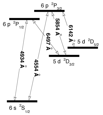
Figure 2: Partial Grotrian diagram of Ba ii showing the levels and the spectral lines of the 5 levels-5 lines model. Note that the level spacings are not to scale.

4 Implication in the Hanle effect diagnostics

First of all, we mention that, since we are not solving the radiative transfer problem, our results have to be considered as complementary informations to the models taking into account radiative transfer without collisions and realistic multilevel models. We introduce the collisional effect together with radiative rates and we determine the emergent fractional polarization in the limit of tangential observation in a plane-parallel atmosphere where the cosine of the heliocentric angle $\mu$ $\simeq$ 0.

If we calculate the polarization in the framework of the 5 levels-5 lines model as a function of the neutral hydrogen density n${}_{\textrm{\scriptsize{H}}}$ (see Fig. 3), one could remark that collisions start to play a notable role for $n_{\textrm{\scriptsize H}}\sim 3\times 10^{13}$ cm^-3. The alignment of the metastable levels ${}^{2}D_{3/2}$ and ${}^{2}D_{5/2}$ start to diminish due to collisions and thus the polarization of the Ba ii line at ${\lambda}4554$ decreases. Indeed, for $n_{\textrm{\scriptsize H}}\sim 3\times 10^{13}$ cm^-3, the ratio of the polarization degree $p$ divided by the zero-collisions polarization $p_{max}$ is $\sim$ 0.9 (i.e. a collisional depolarization of $\sim$ 10%). However, in the framework of the simplified model (Fig. 1), a collisional depolarization of $\sim$ 10% of the ${\lambda}4554$ line is attempted only where $n_{\textrm{\scriptsize H}}\sim 3\times 10^{15}$ cm^-3 (i.e. $\sim$ 100 times larger). This is because the upper level ${}^{2}P_{3/2}$ of the ${\lambda}4554$ line start to be affected by collisions solely for densities n${}_{\textrm{\scriptsize{H}}}>10^{15}$ cm^-3 (see Fig. 3).

An estimate height of formation of the ${\lambda}4554$ line is $h\sim 800$ km which corresponds to a neutral hydrogen density $n_{\textrm{\scriptsize H}}\sim 2\times 10^{14}$ cm^-3 and a temperature of the formation of the lines $T\sim$ 5350K (e.g. model C of Vernazza et al. 1981). In these typical conditions of formation of the Ba ii line at ${\lambda}4554$, the polarization degree calculated using the simplified atomic model of Fig. 1 is practically insensitive to collisions. This may yield, incorrectly, to the conclusion that collisions do not affect the Ba ii line at ${\lambda}4554$. In the contrary, we find that, using the 5 levels-5 lines atomic model, the polarization degree is decreased by $\sim$ 25% because of the collisions. Therefore, the collisions are an important ingredient to quantitatively interpret this line. This is the main conclusion of the present work.

The polarization in the absence of collisions is called $p_{max}$. Since the impact approximation is well satisfied for collisions between neutral hydrogen atoms and perturbed ions in the solar atmosphere, the collisional rates are simply proportional to the hydrogen density (see their analytical expressions in Sect. 3). To study the effect of collisions on the polarization degree, we report in Fig. 3 the variation of the ratio $p/p_{max}$ as a function of the hydrogen density. In Fig. 3, we make together the results obtained for the simplified model (full line) and for a more realistic model (dotted line). We define the percentage of error in evaluating the collisional sensitivity of the ${\lambda}4554$ line as

$$\Delta p=\Big{(}1-({p/p_{max}})_{\textrm{5 levels-5 lines model}}\Big{)}\times 100$$ (28)

In Fig. 3 we present $\Delta p$ for $n_{\textrm{\scriptsize H}}\sim 2\times 10^{14}$ cm^-3.

To assess the sensitivity of the microturbulent magnetic field determination to the collisions, we proceed as follow:

1. In the absence of collisions, we determine the polarization degree $p_{0}$ which corresponds to the critical magnetic field of the Ba ii ${\lambda}4554$ line, $B_{0}\simeq 9$ G.

2. In the absence of collisions, for each value of an eventual collisional inaccuracy $\Delta p$ determined in Eq. (28), the magnetic field $B$ giving the polarization $p=p_{0}\times(1+\Delta p/100)$ is retained. In other words, we introduce a perturbation $\Delta p$ to the polarization $p_{0}$ and we calculate the corresponding magnetic field. We notice that, in general, the effect of the collisions can be overestimated or neglected implying that the polarization should be written generally as $p=p_{0}\times(1\pm\Delta p/100)$. Here, we investigate only the more typical case where the collisions are neglected which corresponds to $p=p_{0}\times(1+\Delta p/100)$.

3. The percentage of error in evaluating the magnetic field due to the neglecting of the collisions is defined by:

   $$\Delta B=\Big{|}1-(B/B_{0})\Big{|}\times 100$$ (29)

   We obtain $\Delta B$ for each value of $\Delta p$ (i.e. for each $n_{\textrm{\scriptsize H}}$). $\Delta B$ reaches the asymptotic value $100\%$ if $B=2B_{0}$ or larger.

The choice of the couple ($B_{0}$, $p_{0}$) as a starting point before perturbing the polarization degree by a $\Delta p$ is arbitrary. An other starting couple should give a rather similar $\Delta B$ provided that the magnetic field is suitable in the sense that it is well included in the domain of sensitivity of the Ba ii ${\lambda}4554$ line to the Hanle effect.

In Fig. 4, we show the percentage of error $\Delta B$ as a function of $n_{\textrm{\scriptsize H}}$. For instance, at $n_{\textrm{\scriptsize H}}\sim 2\times 10^{14}$ cm^-3, where the neglecting of collisions induces an overestimation of the polarization by $\sim$ 25%, the value of the magnetic field is overestimated by $\sim$ 35%. As it could be easily seen in Fig. 4, depolarizing collisions can be neglected for n${}_{\textrm{\scriptsize H}}<\sim 10^{12}$ cm^-3 since the percentage error on the determination of the magnetic field is almost zero. At the asymptotic values of n${}_{\textrm{\scriptsize H}}$ (i.e. n${}_{\textrm{\scriptsize H}}$ $>\sim 10^{17}$ cm^-3), the calculation of the scattering polarization is highly affected by the neglecting of the collisions and the information about the magnetic field is completely lost (the percentage of error is $\sim$ 100%).

Figure 3: Emergent linear polarization amplitudes $p$ divided by the zero-collisions polarization $p_{max}$ versus the density of neutral hydrogen $n_{\textrm{\scriptsize H}}$. (1) Full line: variation of the linear polarization in the framework of the simplified model. (2) Dotted line: same as in (1) but in the framework of the 5 levels-5 lines model.

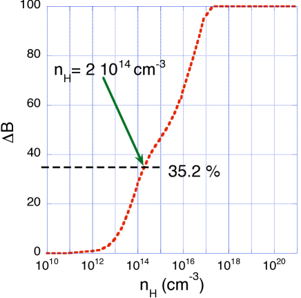
Figure 4: Percentage of error on the magnetic field determination due to the neglecting of the collisions with neutral hydrogen as a function of $n_{\textrm{\scriptsize H}}$.

5 Concluding comments

It is well known that collisions with neutral hydrogen are essential to model the processes governing the formation of many polarized lines in the solar photosphere (D₁ and D₂ lines of Na i; Ti i ${\lambda}4536$; Sr i ${\lambda}4607$; etc). We show in this work that, although the neutral hydrogen is about ten times less abundant in the low chromosphere than in the photosphere, the polarization of the chromospheric ${\lambda}4554$ line decreases significantly due to collisions with hydrogen atoms.

Conclusions about the role of the collisions should not be only based on a simple comparison of the inverse lifetime of the upper level of the transition and the $D^{2}$ coefficients. Although this can give useful indications, realistic conclusion should be inferred only from a full introduction of the depolarization and collisional transfer rates in the SEE for multi-level models.

Lines like Ba ii ${\lambda}4554$ having upper $np$-level energy larger than the energy of the ($n$-1)$d$-level cannot be treated with a simplified model approximation ($n$ is the principal quantum number). For instance, to model quantitatively the K Sr ii ${\lambda}4078$ line one should take into account the alignment of the $d$-sates and the infrared triplet Sr ii ${\lambda}10036$, Sr ii ${\lambda}10327$, and Sr ii ${\lambda}10914$. We notice that the K Sr ii ${\lambda}4078$ line was examined by Bianda et al. (1998), but they used the traditional Van der Waals approach to calculate collisional rates and neglected the collisional depolarization of the long lived $d$-level. Interestingly, although the Mg ii is in the same isoelectronic sequence as Ca ii, Sr ii, and Ba ii, the energy of the upper $p$-level of the K Mg ii ${\lambda}2796$ line is smaller than the energy of the $d$-level. This is fortunate because the modeling of this line could be safely performed using a simplified atomic model neglecting the role of the $d$-level. Furthermore, the K Mg ii ${\lambda}2796$ line is expected to be strongly polarized since the curve showing the anisotropy factor as a function of ${\lambda}$ reaches its maximum around ${\lambda}\sim 2800$ $\AA$ (see Fig. 2 of Manso Sainz & Landi Degl’Innocenti 2002). In addition, in given physical conditions, collisional effects are clearly smaller for Mg ii than for Sr ii and Ba ii. Observations of this line are difficult from the ground-based telescopes but it could be observed with the help of high sensitivity modern polarimeters attached to space missions.

To point out trends in the depth dependence of the magnetic field, Derouich et al. (2006) interpreted spatially-resolved observations of the photospheric Sr i ${\lambda}4607$ line. In order to extend their diagnostic over larger parts of the solar atmosphere, quantitative interpretation of the Ba ii ${\lambda}4554$ line, also observed with spatial resolution, would be highly interesting. To quantitatively study this line, one has to account for partial frequency redistribution effects (e.g. Uitenbroek & Bruls 1992 and Rutten & Milkey 1979). Here also collisions should play an important role since, besides their effects on the atomic polarization, they could change the frequency of the Ba ii photons. It remains a challenge to develop a general theory for partial frequency redistribution of polarized radiation in the presence of arbitrary magnetic fields and including the effects of collisions in a multilevel picture with/without hyperfine structure.

- (1) Belluzzi, L., Trujillo Bueno, J., & Landi Degl’Innocenti, E., 2007, ApJ, 666, 588
- (2) Bianda, M., Stenflo, J. O., & Solanki, S. K., 1998, A&A, 337, 565
- (3) Derouich, M., Sahal-Bréchot, S., & Barklem, P.S., 2004, A&A, 426, 707
- (4) Derouich, M., Bommier, V., Malherbe, J. M., Landi Degl’Innocenti, E., 2006, A&A, 457, 1047
- (5) Derouich, M., Trujillo Bueno, J., Manso Sainz, R., 2007, A&A, 472, 269
- (6) Landi Degl’Innocenti, E., & Landolfi, M., 2004, Polarization in Spectral Lines (Dordrecht: Kluwer)
- (7) López Ariste, A., Asensio Ramos, A., Manso Sainz, R., Derouich, M., Gelly, B., A&A, in revision
- (8) Malherbe, J. M., Moity, J., Arnaud J., & Roudier, Th., 2007, A&A, 462, 753
- (9) Manso Sainz, R., & Landi Degl’Innocenti, E., 2002, A&A, 394, 1093
- (10) Rutten, R. J. & Milkey, R. W., 1979, ApJ, 231, 277
- (11) Tandberg-Hanssen, E., & Smythe, C., 1970, ApJ, 161, 289
- (12) Trujillo Bueno J., 2001, in Advanced Solar Polarimetry: Theory, Observation and Instrumentation, ed. M. Sigwarth, ASP Conf. Series 236, 161
- (13) Vernazza J. E., Avrett E. H., Loeser R., 1981, ApJS, 45, 635
- (14) Uitenbroek, H. & Bruls, J. H. M. J., 1992, A&A, 265, 268
- (15) Unsöld A.L., 1927, Zeitschrit für Physik, 43, 574
- (16) Unsöld A.L., 1955, Physik der Stern Atmosphären (Zweite Auflage)