Entropy landscape and non-Gibbs solutions in constraint satisfaction problems

Abstract

We study the entropy landscape of solutions for the bicoloring problem in random graphs, a representative difficult constraint satisfaction problem. Our goal is to classify which type of clusters of solutions are addressed by different algorithms. In the first part of the study we use the cavity method to obtain the number of clusters with a given internal entropy and determine the phase diagram of the problem, e.g. dynamical, rigidity and SAT-UNSAT transitions. In the second part of the paper we analyze different algorithms and locate their behavior in the entropy landscape of the problem. For instance we show that a smoothed version of a decimation strategy based on Belief Propagation is able to find solutions belonging to sub-dominant clusters even beyond the so called rigidity transition where the thermodynamically relevant clusters become frozen. These non-equilibrium solutions belong to the most probable unfrozen clusters.

I Introduction and Motivations

Many disciplines have at their root random Constraint Satisfaction Problems (CSPs). Examples are Information Theory where they are used to design error correcting codes G-book-1968 ; M-book-2002 or Computer Science where they constitute elementary models for studying the onset of exponential regimes in algorithmsDMSZ-tcs-2001 . More in general, random CSPs capture some of the optimization aspects of complex systems found in physics (e.g. spin-glasses and packing problems), in economics (e.g. financial markets)CMZ-prl-2000 ; GLMSWZ-prl-2006 and in biology (e.g. gene networks reconstruction and learning in neuroscience BZ-prl-2006 ; BBBZ-pnas-2007 ). A random CSP is characterized by an extensive list of constraints, each one forbidding some of the joint assignments of the (discrete) variables it involves. In packing problems for instance, overlapping positions of the elementary tiles on a given lattice are forbidden. Given an instance of a CSP, one wants to know whether there exists a solution, that is an assignment of the variables which satisfies all the constraints (e.g. a proper tiling or a proper coloring of a graph). When such assignment exists the instance is called SAT, and one wants to find it. Most of the interesting CSPs are NP-completeC-acm-1971 ; GJ-book-1979 : in the worst case the number of operations needed to decide whether an instance is SAT or not is expected to grow exponentially with the number of variables. The interesting limit for random CSP is the thermodynamic one where both the number $N$ of independent variables and the number $M$ of constraints go to infinity at fixed constraint density $\alpha\equiv M/N$. The most intriguing phenomenon is certainly the appearance of sharp thresholds KS-science-1994 ; MZKST-nature-1999 . At some critical ratio $\alpha_{s}$ the probability of existence of solutions jumps from one to zero. Just below such threshold, most of the known heuristic algorithms are observed to undergo a dramatic slowing down. Such phenomenon has been put in connection with the onset of a clustering phase, where the space of solution becomes divided in a large (exponential) number of different clusters (or states) and variables develop non trivial long range correlations.

Scope of this study is to go a step further in the statistical physics analysis of the connection between clustering and the behavior of algorithms. By an analytic estimate of the internal entropy of the clusters found by different algorithms on large problem instances, and by a large deviation analysis of clusters distribution with respect to their internal entropy, we are able to display which type of clusters are addressed by different algorithms. For random CSP in the clustering phase, we observe that local search algorithms may be attracted by a large spectrum of clusters (not surprisingly as it happens in out-of-equilibrium physical systems). Quite surprisingly we also show that there exist simple message-passing (MP) processes that are capable of finding efficiently solutions even in the harder region where the thermodynamically dominant clusters become frozen. In such region local search algorithms are observed numerically to undergo an exponential slowing down due to the global rearrangements needed to correct the errors made along the search process. On the contrary, the MP processes that we study continue to find solution efficiently by addressing clusters which are more rare than the dominating ones (i.e. those which would be seen by sampling solutions with uniform measure over the solution space). These results, together with the evidence coming from fully connected CSP that even frozen solutions may be found by MP BZ-prl-2006 , shed new light on how MP algorithms can be utilized and suggest that some further algorithmic progress may be at hand.

In what follows we first provide a very brief review of the known results and next apply our arguments to the so called Bicoloring problem, which has some analytical advantages compared to other NP-complete problems like K-SAT or Coloring while retaining all the conceptual features.

The paper is organized as follows. In sect. II an intuitive introduction to clustering is given. The definition of the specific problem under study is provided in section III together with a summary of previously known results. The cavity method for large deviations is presented in section IV. The numerical methods used to solve the cavity equations and extract the complexity curves are described in section V. In section VI the equations are solved in some special cases in order to obtain the main properties of the phase diagram of the problem. The algorithms used to find solutions and locate them in the entropy landscape are described in section VII. Section VIII is devoted to summarize the main results of the paper and to make some concluding remarks and discuss perspectives. In the appendices we report the details of deriving the cavity equations and some quantities that are essential in computing the free energy.

II Geometry of solutions and freezing

The set of solutions of a random CSP should be thought of as a portion of the phase space which may undergo a fragmentation into clusters for values of the density of constraints right below the SAT threshold. This scenario can be made rigorous in few cases, the simplest one being the random XOR-SAT problemMRZ-jstatphys-2003 ; CDMM-prl-2003 : the density of constraints were clustering appears corresponds to the percolation of particular structures in the underlying graph of constraints. This fact can be used to define clusters which, by linearity of XOR-SAT, turn out to be all identical. One may prove that a finite fraction of the variables have to be frozen, that is must take the same value in all the solutions belonging to a cluster. This picture is however far from general: both the definition of clusters and the analysis of their fluctuations in size are difficult tasks, which require the application of the cavity method in a rather advanced setting MPR-prl-2005 ; M-thesis ; KMRSZ-pnas-2007 ; ZK-arxiv-2007 ; S-arxiv-2007 . One important feature of clusters in CSPs concerns the presence or absence of frozen variables. It may happen that clusters with frozen variables coexist with totally unfrozen clusters of larger internal entropy, with big effects on the hardness of the associated combinatorial optimization problem. The intuitive reason why the presence of frozen variables is believed to be relevant is well summarized by the idea of rearrangements S-arxiv-2007 : ”given an initial solution of a CSP and a variable $i$ that one would like to modify, a rearrangement is a path in configuration space that starts from the initial solution and leads to another solution where the value of the $i$-th variable is changed with respect to the initial one. The minimal length of such a path is a measure of how constrained was the variable $i$ in the initial configuration. In intuitive terms this length diverges with the system size when the variable was frozen in the initial cluster”. The idea is that when freezing takes place in Gibbs states, then the rearrangements are responsible for a critical slowing down of local search algorithms. On the contrary, when dominant clusters are not frozen, even relatively simple local algorithms may find solutions by incrementally adding constraints until the full problem is satisfied. Recent arguments and numerical studies, have shown that one can still obtain a solution beyond the dynamical transition as long as the so-called jamming transition has not occurred KK-arxiv-2007 . Following Ref. KK-arxiv-2007 , one can imagine adding the constraints one by one, in each step recording the number of flips that are required in order to find the new solution. Close to the jamming transition the number of flips diverges and makes it difficult to find a solution to the CSP S-arxiv-2007 .

A Constrained Satisfaction Problem is defined by a set of constrains $\mathcal{C}=\{I_{a}[\underline{\sigma}]\in\{0,1\}|a=1,\ldots,M\}$ on a number of variables. The constraints depend on the configuration of variables $\underline{\sigma}\equiv\{\sigma_{i}|i=1,\cdots,N\}$ and the problem is called satisfiable if all constraints are satisfied, i.e. $I_{a}=1,\forall a$. A solution of the problem is a configuration of the variables that satisfies all constraints. In analogy with statistical physics models, we define the energy $E[\underline{\sigma}]$ of configuration $\underline{\sigma}$ as the number of unsatisfied constraints in $\underline{\sigma}$. Given an instance of a CSP, one is interested in deciding whether it is satisfiable (i.e. $E[\underline{\sigma}]=0$) and, in such a case, in explicitly finding solutions to the problem.

More in general, one can define an ensemble of instances of the problem considering all possible random assignments of the $M$ constraints among $N$ variables, with fixed density of constraints $\alpha=M/N$. Varying $\alpha$ it was shown that the system passes from a phase in which it is always possible to find a solution, the SAT phase, to the UNSAT phase where a fraction of the constraints are not satisfied. Examples of studies for root problems such as Random Satisfiability Problem, XOR-SAT and Graph Coloring can be found in MZ-pre-1997 ; MPZ-science-2002 ; MZ-pre-2002 ; MPWZ-prl-2002 ; ANP-nature-2005 ; MMZ-rsa-2006 . The main tool for analyzing the satisfiability of typical problem instances is the cavity method, originally developed to study the thermodynamic properties of diluted spin-glass systems MPV-1987 and recently reconsidered in the context of CSPs MP-epjb-2001 ; MP-jstatphys-2003 ; MZ-pre-2002 . Actually, the cavity method at the ensemble level allows to study the typical properties as well as large deviations from typical behaviors R-jstatmech-2005 ; MPR-prl-2005 ; KMRSZ-pnas-2007 . The key feature of the cavity method which is of interest for computer science stems from the discovery that it can be converted to an algorithm for analyzing single problem instances MZ-pre-2002 ; BMZ-rsalgorithm-2005 , becoming an efficient solver for the random combinatorial problems.

III Definition of the problem and known results

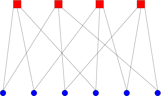
Figure 1: A regular random factor graph with function nodes (squares) of degree $K=3$ and variable nodes (circles) of degree $L=2$.

Consider a hypergraph of $N$ nodes $i=1,\ldots,N$ and $M$ hyperedges $a=1,\ldots,M$. For simplicity we consider regular random hypergraphs, or $(K,L)$-hypergraphs, where each hyperedge connects $K$ nodes and each node contributes in $L=KM/N=K\alpha$ hyperedges. A node in this hypergraph has state $\sigma_{i}\in\{0,1\}$ and each hyperedge imposes a constraint on the values of the associated variables. In the bicoloring problem this constraint just forbids the configurations in which all the nodes belonging to an hyperedge have the same value. In the context of circuit logic the bicoloring problem is known as Not-All-Equal-Satisfiability (NAE-SAT) problem, in physics it is a spin model with anti-ferromagnetic interactions.

We may represent bicoloring as a factor graph KFL-ieee-2001 . This is a bipartite graph where the variables and constraints are represented with two different types of nodes, variable and function nodes, respectively. Each function node is connected to all the variable nodes that should satisfy the associated constraint. Figure 1 shows an example of regular random factor graph.

The hypergraph bicoloring problem is NP-complete for $K\geq 3$ F-jam-1999 . The case $K=3$ with a Poisson degree distribution for the variable nodes has already been studied in CNRZ-jphysa-2003 . The authors found dynamical and SAT/UNSAT transitions within the single and multiple cluster approximations. In spin glass language these approximations are called replica symmetric (RS) and one-step replica symmetry breaking (1RSB) approximation, respectively. In the latter case the authors only consider the most numerous clusters.

$K$	$L^{0}_{d}$	$L_{s}^{RS}$	$L_{s}^{1RSB}$
$3$	$-$	$8$	$7$
$4$	$17$	$21$	$20$
$5$	$40$	$54$	$53$
$6$	$91$	$131$	$130$
$7$	$200$	$309$	$307$
$8$	$428$	$708$	$705$
$9$	$905$	$1594$	$1592$
$10$	$1894$	$3546$	$3543$

Table 1: Numerical values of $L^{0}_{d}$ and $L_{s}$ (in the RS and 1RSB approximations). In each case we have given the smallest integer degree larger than or equal to the precise value.

The intensive entropy $s$ is defined by the number of solutions $\mathcal{N}=e^{Ns}$. Using Bethe approximation in the replica symmetric phase we find the entropy as

$$s^{RS}=\ln[2(1-\frac{1}{2^{K-1}})^{L}]-(K-1)\alpha\ln[1-\frac{2}{2^{K}}].$$ (1)

This quantity vanishes at

$$L_{s}^{RS}=-K\frac{\ln 2}{\ln(1-\frac{1}{2^{K-1}})},$$ (2)

where for $K\gg 1$ gives

$$L_{s}^{RS}\simeq K2^{K-1}\ln 2(1+O(\frac{1}{2^{K}})).$$ (3)

If there exist more than one cluster of solutions we define the complexity $\Sigma$ by $\mathcal{N}_{c}=e^{N\Sigma}$ where $\mathcal{N}_{c}$ is the number of clusters. Notice that for very large $N$ the above complexity is dominated by typical clusters. In 1RSB approximation and considering only typical clusters, the complexity reads CNRZ-jphysa-2003 ,

$$\Sigma_{typ}=\ln[A_{L}]-(K-1)\alpha\ln[1-\frac{1}{2}(1-\eta)(1-\frac{\eta^{L-1}}{A_{L-1}})],$$ (4)

where

$$A_{L}=2(1-\frac{1-\eta}{2})^{L}-\eta^{L},$$ (5)

and $\eta$ is determined by the following equation

$$\eta=1-2[\frac{1}{2}(1-\frac{\eta^{L-1}}{A_{L-1}})]^{K-1}.$$ (6)

A nontrivial solution ($\eta\neq 1$) for the above equation results to a nonzero complexity. Let us assume $K\gg 1$ and find the point where for the first time a nontrivial solution appears. We try $\eta=1-\frac{c}{2^{K-1}}$ and find $c$ in a self-consistent way. From the above equation we obtain

$$\frac{c}{2}\simeq\exp[-\frac{K-1}{2}e^{-c\frac{L-1}{2^{K}}}].$$ (7)

It means that to have a finite solution for $c$ we need $L$ diverges as

$$L^{0}_{d}\simeq 2^{K}\frac{1}{c}[\ln K-\ln 2-\ln\ln(\frac{2}{c})+o(1)].$$ (8)

At the SAT/UNSAT transition $\Sigma_{typ}$ vanishes and we can use this fact to determine $\alpha_{s}$. This value behaves, asymptotically, as $\alpha_{s}^{RS}$ in Eq. 3. In table 1 we compare the numerical values of $L_{d}^{0}$ and $L_{s}$ obtained with the above methods.

IV Cavity method: a large deviation study

A more complete picture of the distribution of clusters is given by a large deviation study R-jstatmech-2005 ; MPR-prl-2005 ; KMRSZ-pnas-2007 . We define the partition function at zero temperature as

$$Z=\sum_{\underline{\sigma}}\prod_{a}I_{a}(\sigma_{\partial a})e^{x\sum_{i}(\sigma_{i}-\sigma_{i}^{*})^{2}}.$$ (9)

Here $x$ is a Lagrange multiplier that controls the distance between the solutions and a reference point $\underline{\sigma}^{*}$. And $\sigma_{\partial a}=\{\sigma_{i}|i\in V(a)\}$ where $V(a)$ is the set of neighbors of function node $a$. For $x=0$ we recover the total number of solutions. If there is only one cluster of solutions we can safely use the standard Belief Propagation (BP) equations KFL-ieee-2001 to obtain an estimate of the cavity marginals (see appendix A)

$$\mu_{i\rightarrow a}(\sigma_{i})=\frac{1}{Z_{i\rightarrow a}}\sum_{\sigma_{\partial i\rightarrow a}}\left(\prod_{b\in V(i)\setminus a}I_{b}(\sigma_{\partial b})[\prod_{j\in V(b)\setminus i}\mu_{j\rightarrow b}(\sigma_{j})]\right)e^{x(\sigma_{i}-\sigma_{i}^{*})^{2}}.$$ (10)

Here $Z_{i\rightarrow a}$ is a normalization constant, $V(i)$ is the set of neighbors of variable node $i$ and $\sigma_{\partial i\rightarrow a}=\{\sigma_{j}|j\in V(b),b\in V(i)\setminus a\}$. We will write the above equation in short as

$$\mu_{i\rightarrow a}(\sigma_{i})=\mathcal{S}[\mu_{j\rightarrow b}].$$ (11)

We also define the free energy $f(x)$ as

$$Z=e^{Nf(x)}=\sum_{d}e^{N[s(d)+xd]},$$ (12)

where $d=\frac{1}{N}\sum_{i}(\sigma_{i}-\sigma_{i}^{*})^{2}$ and $e^{Ns(d)}$ is the number of solutions at distance $d$ from the reference point. In the Bethe approximation

$$f(x)=\sum_{i}\Delta f_{i}-\sum_{a}(K_{a}-1)\Delta f_{a},$$ (13)

where

$$e^{N\Delta f_{i}}=\sum_{\sigma_{i}}[\prod_{a\in V(i)}\mu_{a\rightarrow i}(\sigma_{i})]e^{x(\sigma_{i}-\sigma_{i}^{*})^{2}},$$ (14)

$$e^{N\Delta f_{a}}=\sum_{\sigma_{\partial a}}I_{a}(\sigma_{\partial a})\prod_{i\in V(a)}\mu_{i\rightarrow a}(\sigma_{i}).$$

Using the above free energy we can determine the entropy $s(d)$ by a Legendre transform

$$s(d)=\min_{x}{[f(x)-xd(x)]},\hskip 28.45274ptd(x)=\frac{\partial f(x)}{\partial x}.$$ (15)

If the replica symmetry is broken, we would have different clusters of solutions and the cavity marginals fluctuate from one cluster to another one. This is described by a generalized partition function defined by

$$\mathcal{Z}\equiv e^{N\mathcal{F}(m)}=\sum_{c}e^{mNs_{c}}=\int dse^{N[\Sigma(s)+ms]}.$$ (16)

Here $c$ labels the clusters and $s_{c}$ is the internal entropy of cluster $c$. Again in the Bethe approximation

$$N\mathcal{F}(m)=\sum_{i}\ln\mathcal{Z}_{i}-\sum_{a}(K_{a}-1)\ln\mathcal{Z}_{a}$$ (17)

where

$$\mathcal{Z}_{i}\equiv\int\prod_{a\in V(i)}\prod_{j\in V(a)\setminus i}d\mathcal{P}_{j\rightarrow a}[\mu_{j\rightarrow a}]e^{mN\Delta s_{i}},$$ (18)

$$\mathcal{Z}_{a}\equiv\int\prod_{i\in V(a)}d\mathcal{P}_{i\rightarrow a}[\mu_{i\rightarrow a}]e^{mN\Delta s_{a}}.$$

Having the generalized free energy we can determine the complexity $\Sigma(s)$ by a Legendre transformation

$$\Sigma(s)=\min_{m}{[\mathcal{F}(m)-ms]},\hskip 28.45274pts(m)=\frac{\partial\mathcal{F}(m)}{\partial m}.$$ (19)

In appendix B we have explained the origin of the above relations. Notice that $\Delta s_{i}=\Delta f_{i}(x=0)$ and $\Delta s_{a}=\Delta f_{a}(x=0)$, where the free energy shifts are given by Eq. 14. Moreover, $\mathcal{P}_{i\rightarrow a}[\mu_{i\rightarrow a}]$ is the probability that, in a randomly selected cluster, we find the cavity marginal $\mu_{i\rightarrow a}$ on edge $(i,a)$ of the factor graph. This probability distribution is determined by the following self-consistency equation:

$$\mathcal{P}_{i\rightarrow a}[\mu_{i\rightarrow a}]=\frac{1}{\mathcal{Z}_{i\rightarrow a}}\int\prod_{b\in V(i)\setminus a}\prod_{j\in V(b)\setminus i}d\mathcal{P}_{j\rightarrow b}[\mu]e^{mN\Delta s_{i}}\delta(\mu_{i\rightarrow a}-\mathcal{S}[\mu]),$$ (20)

where $\mathcal{Z}_{i\rightarrow a}$ is a normalization constant and $\mathcal{S}[\mu]$ is the same as in Eq. 11 with $x=0$. The factor $e^{mN\Delta s_{i}}$ is to sample correctly the clusters when we add the new variable $i$. Let us multiply the two sides of Eq. 20 by $2\mu_{i\rightarrow a}(\sigma)$, to find the new probability distribution $\mathcal{Q}_{i\rightarrow a}^{\sigma}[\mu]=2\mu_{i\rightarrow a}(\sigma)\mathcal{P}_{i\rightarrow a}[\mu]$ that will be useful in the special case of $m=1$. In the right hand side we can replace $\mu_{i\rightarrow a}(\sigma)$ with its definition in Eq. 10. Rearranging the terms we get

$$\mathcal{Q}_{i\rightarrow a}^{\sigma_{i}}[\mu]=\frac{2}{\mathcal{Z}_{i\rightarrow a}}\int\sum_{\sigma_{\partial i\rightarrow a}}\prod_{b\in V(i)\setminus a}I_{b}(\sigma_{\partial b})\prod_{j\in V(b)\setminus i}\left(\frac{1}{2}d\mathcal{Q}_{j\rightarrow b}^{\sigma_{j}}[\mu]\right)e^{(m-1)N\Delta s_{i}}\delta(\mu_{i\rightarrow a}-\mathcal{S}[\mu]).$$ (21)

In the following we will split $\mathcal{P}_{i\rightarrow a}[\mu]$ into frozen and unfrozen parts as

$$\mathcal{P}_{i\rightarrow a}[\mu_{i\rightarrow a}]=\frac{1-\pi}{2}[\delta(r)+\delta(r-1)]+\pi\rho(r),$$ (22)

where $\mu_{i\rightarrow a}(0)=r$, $\mu_{i\rightarrow a}(1)=1-r$ and $\rho(r)$ is the probability distribution of unfrozen fields. The above arguments become much simpler in random $(K,L)$-hypergraphs where all the links and nodes are statistically equivalent. For example, Eq. 17 is replaced with

$$\mathcal{F}(m)=\ln[\int D_{i}\mathcal{P}[\mu]e^{mN\Delta s_{i}}]-\alpha(K-1)\ln[\int D_{a}\mathcal{P}[\mu]e^{mN\Delta s_{a}}],$$ (23)

where $\int D_{i}\mathcal{P}[\mu]$ and $\int D_{a}\mathcal{P}[\mu]$ denote the integrations over all the cavity marginals that contribute in $\Delta s_{i}$ and $\Delta s_{a}$, respectively.

V Entropy landscape: Numerical method

The main equation that we should solve is Eq.20. One can use the population dynamics method MP-epjb-2001 ; MP-jstatphys-2003 to get rid of summing over a large number of continuous variables.

V.1 In a single hypergraph

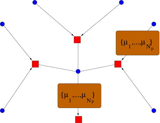
Figure 2: Population dynamics works with a population of fields on each link of the factor graph.

Given the factor graph we represent $\mathcal{P}_{i\rightarrow a}[\mu]$ by a population of $\mathcal{N}_{p}$ cavity probabilities (or fields), Fig. 2. At the initial point all the cavity fields are of frozen kind, with equal probability for $r=0$ and $r=1$. With this initial condition we will not miss a nontrivial solution with frozen fields, if any. At each step of the population dynamics we select a link $(i\rightarrow a)$ randomly and do in the following way:

• For each $b\in V(i)\setminus a$ and $j\in V(b)\setminus i$: randomly select a member of the population on link $(j\rightarrow b)$.

• Using these $(L-1)(K-1)$ fields: calculate the new $\mu_{i\rightarrow a}$ by Eq. 10.

• Calculate the weight $w_{i\rightarrow a}=e^{mN\Delta s_{i}}$ from Eq. 14 at $x=0$. This weight is zero if there is any contradiction.

• With probability $\frac{w_{i\rightarrow a}}{w^{max}_{i\rightarrow a}}$ replace a randomly selected member of the population with the new one. Here $w^{max}_{i\rightarrow a}$ is the maximum weight $w_{i\rightarrow a}$ observed in the evolution from the beginning.

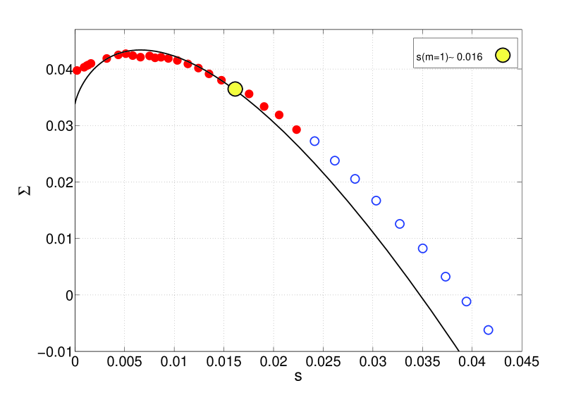
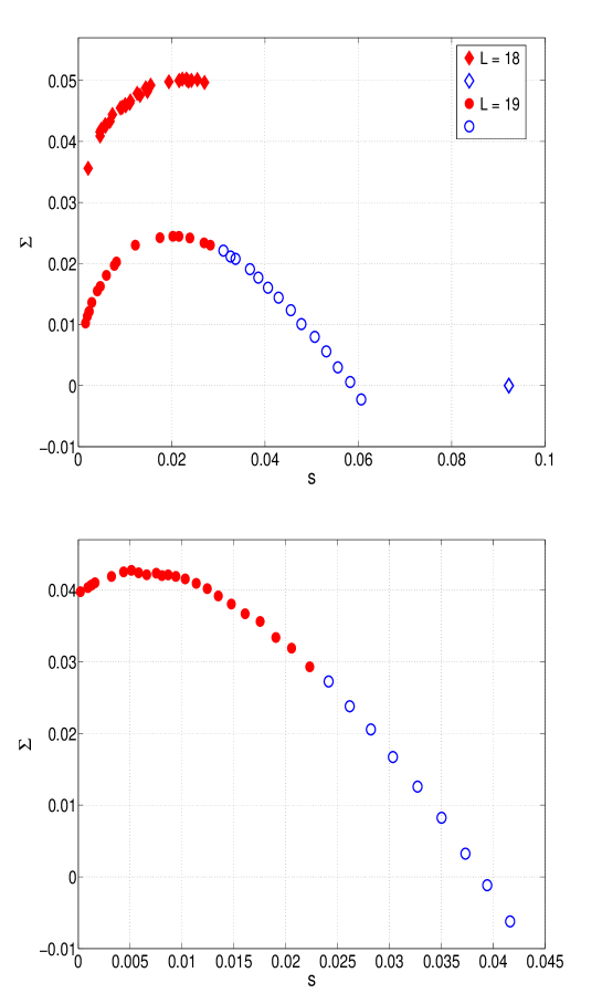
Figure 3: Complexity vs entropy for $K=4$, $L=18,19$ with $\mathcal{N}_{p}=10^{5}$ (top) and $K=6$, $L=121$ with $\mathcal{N}_{p}=2\times 10^{4}$ (bottom) in one-link approximation . Filled and empty symbols represent frozen and unfrozen parts, respectively. The statistical errors are about $0.001$.

In a sweep of the algorithm we choose all the links of the factor graph randomly. Having the populations we can obtain the free energy as

$$N\mathcal{F}(m)=\sum_{i}\ln\mathcal{Z}_{i}-(K-1)\sum_{a}\ln\mathcal{Z}_{a},$$ (24)

$$\mathcal{Z}_{i}=\langle e^{mN\Delta s_{i}}\rangle_{pop},$$

$$\mathcal{Z}_{a}=\langle e^{mN\Delta s_{a}}\rangle_{pop},$$

where $\langle.\rangle_{pop}$ means averaging over the populations. We stop the updates as soon as the free energy, and so the weights $w^{max}_{i\rightarrow a}$, reach the steady state. Then the entropy reads

$$Ns(m)=\sum_{i}\overline{\Delta s_{i}}-(K-1)\sum_{a}\overline{\Delta s_{a}},$$ (25)

$$\overline{\Delta s_{i}}=\frac{\langle\Delta s_{i}e^{mN\Delta s_{i}}\rangle_{pop}}{\langle e^{mN\Delta s_{i}}\rangle_{pop}},$$

$$\overline{\Delta s_{a}}=\frac{\langle\Delta s_{a}e^{mN\Delta s_{a}}\rangle_{pop}}{\langle e^{mN\Delta s_{a}}\rangle_{pop}}.$$

Figure 3 shows the results for choices of the factor graph parameters that correspond to different phases.

V.2 In one-link approximation

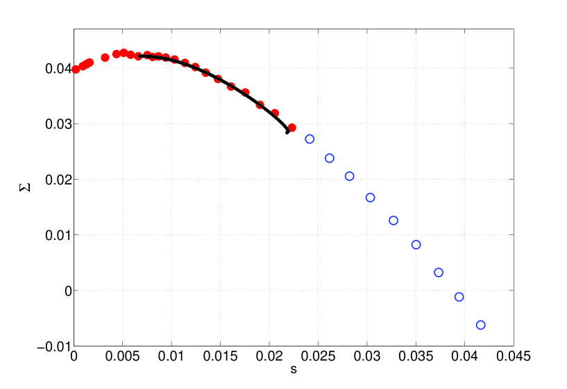
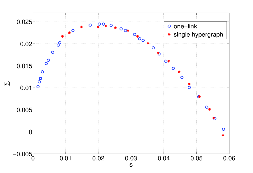
In a regular random hypergraph all links of the associated factor graph are equivalent. Therefore we can forget about different populations on different links and work with only one large population of fields. The way we obtain the stationary distribution $\mathcal{P}[\mu]$ is the same as above. The only difference is that we always select the fields from the single population. In Fig. 4 we compare the complexity computed on a single $(4,19)$-hypergraph of size $N=10^{4}$ with the complexity obtained in the one-link approximation.

Figure 4: Comparing $\Sigma(s)$ in a single $(4,19)$-hypergraph ($N=10^{4}$, $\mathcal{N}_{p}=10^{2}$) and in one-link approximation with $\mathcal{N}_{p}=10^{5}$. The statistical errors are about $0.001$.

VI Entropy landscape: Analytical results

To locate different phase transitions in the solution space we need to calculate the generalized free energy $\mathcal{F}$ which is given in terms of $\mathcal{Z}_{i}$ and $\mathcal{Z}_{a}$ in Eq. 18. These quantities in turn depend on the fraction of frozen variables $\pi$ and $\rho(r)$ which should be determined by Eq. 20 for $\mathcal{P}[\mu]$. In the following we study some special cases that allow us to calculate the above quantities and determine the phase diagram of the problem. For clarity here we only state the results of calculations that will be presented in more details in appendix C.

VI.1 The case $m=1$

The study of $m=1$ clusters is relevant in determining the dynamical, rigidity and condensation transitions KMRSZ-pnas-2007 . These are in fact the thermodynamically relevant clusters before the condensation transition.

For $m=1$ the generalized free energy reads

$$\mathcal{F}=\ln\left(2[1-\frac{1}{2^{K-1}}]^{L}\right)-(K-1)\alpha\ln\left(1-\frac{2}{2^{K}}\right).$$ (26)

Comparing with the RS entropy $s^{RS}$ in Eq. 1 we see that $\mathcal{F}(m=1)=\Sigma(m=1)+s(m=1)=s^{RS}$. Therefore, as long as the $m=1$ clusters are the thermodynamically relevant ones the RS approximation gives the correct total entropy. From Eq. 21 we can also find the probability of having a frozen field with $r=1$

$$\frac{1-\pi}{2}=\frac{1}{\mathcal{Z}_{i\rightarrow a}}\left([1-\frac{1}{2^{K-1}}]^{L-1}-[1-\frac{1}{2^{K-1}}-(\frac{1-\pi}{2})^{K-1}]^{L-1}\right).$$ (27)

For small $L$ the above equation has only one solution, $\pi=1$, where the $m=1$ clusters are unfrozen. Increasing $L$, one reaches the rigidity point $L_{r}$ where another solution $\pi\neq 1$ appears. It is where a finite fraction of the variables in these clusters become frozen. We find that for $K<6$ the rigidity transition always happens after the SAT/UNSAT transition. Simplifying the above equation we obtain

$$\pi=[1-\frac{(\frac{1-\pi}{2})^{K-1}}{1-\frac{1}{2^{K-1}}}]^{L-1}.$$ (28)

Assuming $K\gg 1$ and $\pi=\frac{c}{K}$ one obtains

$$c\simeq K\exp[-\frac{(L-1)}{2^{K-1}}e^{-c}],$$ (29)

which suggests

$$L_{r}\simeq 2^{K-1}e^{c}[\ln K-\ln c+o(1)].$$ (30)

We see that, like $L_{d}^{0}$, the leading term in $L_{r}$ diverges as $2^{K}\ln K$. Compare it with the leading term of $L_{s}^{RS}$ which scales as $2^{K}K$.

VI.2 The case $m=0$

The typical or most numerous clusters are the $m=0$ ones. The study of these clusters provides us with an estimate of the SAT/UNSAT transition (in that they are the last clusters to disappear). Indeed the previous studies of the complexity in 1RSB phase focus on these type of clusters. For $m=0$ the generalized free energy reads

$$\mathcal{F}=\ln\left(2[1-(\frac{1-\pi}{2})^{K-1}]^{L}-[1-2(\frac{1-\pi}{2})^{K-1}]^{L}\right)-(K-1)\alpha\ln\left(1-2(\frac{1-\pi}{2})^{K}\right).$$ (31)

Using Eq. 20 one can easily write an equation for the fraction of frozen marginals

$$\frac{1-\pi}{2}=1-\frac{[1-(\frac{1-\pi}{2})^{K-1}]^{L-1}}{2[1-(\frac{1-\pi}{2})^{K-1}]^{L-1}-[1-2(\frac{1-\pi}{2})^{K-1}]^{L-1}}.$$ (32)

The above equation is another way of writing Eq. 6 that has been obtained in the previous studies. Notice that

$$\pi=\frac{\eta^{L-1}}{A_{L-1}},$$ (33)

with $A_{L-1}$ and $\eta$ given by Eqs. 5 and 6. A nontrivial solution for $\pi$ appears at $L^{0}_{d}$, where for the first time a maximum appears in the curve $\Sigma(s)$. According to Eq. 19 the complexity of $m=0$ clusters is $\Sigma(m=0)=\mathcal{F}$. The point that this quantity vanishes defines the SAT/UNSAT transition $L_{s}$. One can show that, like $L_{s}^{RS}$, the leading term in $L_{s}$ scales as $2^{K}K$.

VI.3 The case $\pi=0$

Figure 5: Comparing $\Sigma(s)$ for $K=6$ and $L=121$ (in one-link approximation with $\mathcal{N}_{p}=2\times 10^{4}$) with $\Sigma(s,\pi=0)$.

This case is relevant to study very small clusters or close to the SAT/UNSAT transition where almost all variables are frozen and $\pi\simeq 0$. Notice that solving numerically for $\Sigma(s)$ is a heavy computational job and it would be useful to have other approximation methods to get a good estimate of the complexity. When $\pi=0$ the generalized free energy is given by

$$\mathcal{F}=\ln\left(2(2^{m-1}-1)[1-\frac{2}{2^{K-1}}]^{L}+2[1-\frac{1}{2^{K-1}}]^{L}\right)-(K-1)\alpha\ln\left(1-\frac{2}{2^{K}}\right).$$ (34)

Taking derivatives we obtain the entropy as

$$s=\frac{2^{m}[1-\frac{2}{2^{K-1}}]^{L}\ln 2}{2(2^{m-1}-1)[1-\frac{2}{2^{K-1}}]^{L}+2[1-\frac{1}{2^{K-1}}]^{L}}.$$ (35)

With the above quantities we can obtain the complexity of different clusters. In Fig. 5 we have compared this complexity with the one obtained numerically in the one-link approximation. As the figure shows the agreement is good especially for the smaller and frozen clusters.

Close to the condensation transition the $m=1$ clusters are nearly completely frozen and we expect the $\pi=0$ complexity to give a good estimate of $\Sigma(m=1)$. From the above equations we obtain

$$\Sigma(m=1)\simeq\ln\left(2[1-\frac{1}{2^{K-1}}]^{L}\right)-(K-1)\alpha\ln\left(1-\frac{2}{2^{K}}\right)-\left(\frac{1-\frac{2}{2^{K-1}}}{1-\frac{1}{2^{K-1}}}\right)^{L}\ln 2.$$ (36)

We use this approximated complexity to determine the condensation transition, $L_{c}$, where $\Sigma(m=1)$ vanishes. After some algebra we find that for $K\gg 1$

$$L_{c}\simeq K2^{K-1}(\ln 2-\frac{K}{2^{K}}+o(1)).$$ (37)

Notice that the leading term in $L_{c}$ is exactly the same as in $L_{s}^{RS}$.

VI.4 The case $\pi=1$

The complexity can be nonzero even when the frozen fields are absent. In this case we can exactly compute the free energies of $m=0,1,2$ clusters. We use this fact to find an approximated free energy for $m\in[0,2]$. Having $\mathcal{F}(m=0)$, $\mathcal{F}(m=1)$ and $\mathcal{F}(m=2)$ we use the Lagrange interpolating polynomial function to write $\mathcal{F}(m)$ around $m=1$

$$\mathcal{F}(m)=-\mathcal{F}(m=1)m(m-2)+\mathcal{F}(m=2)\frac{m(m-1)}{2},$$ (38)

where we have used the fact that for $\pi=1$, $\mathcal{F}(m=0)=0$. The resulted entropy and complexity are

$$s(m)=-2(m-1)\mathcal{F}+(m-\frac{1}{2})\mathcal{F}(m=2)$$ (39)

$$\Sigma(m)=m^{2}[\mathcal{F}(m=1)-\frac{1}{2}\mathcal{F}(m=2)].$$

As we show in appendix C, the free energy $\mathcal{F}(m=2)$ depends on the second moment of the $\rho(r)$,

$$\langle r^{2}\rangle=\frac{1}{\mathcal{Z}_{i\rightarrow a}(m=2)}[1-\frac{2}{2^{K-1}}+\langle r^{2}\rangle^{K-1}]^{L-1}.$$ (40)

It turns out that $\Sigma(m=1)$ is zero as long as $\langle r^{2}\rangle=1/4$, i.e. $\rho(r)=\delta(r-\frac{1}{2})$. The complexity becomes nonzero only when equation 40 suggests a nontrivial solution. We can rewrite Eq. 40 as

$$x=[1-\frac{1-x^{K-1}}{1+(1+x)^{K-1}(2^{K-1}-2)}]^{L-1},x\equiv\frac{1}{2\langle r^{2}\rangle}-1.$$ (41)

Taking $K\gg 1$ and $x=\frac{c}{K}$ we find

$$c\simeq K\exp[-\frac{L}{2^{K-1}}e^{-c}].$$ (42)

The equation suggests that

$$L_{d}\simeq 2^{K-1}e^{c}[\ln K-\ln c+o(1)],$$ (43)

which behaves very similar to $L_{d}^{0}$ in Eq. 8.

VI.5 The case of integer $m$

Figure 6: Comparing $\Sigma(s)$ for $K=6$ and $L=121$ (in one-link approximation with $\mathcal{N}_{p}=2\times 10^{4}$) with the complexity that has been obtained by interpolation approximation ($N_{m}=10$).

Suppose that we have computed $\mathcal{Z}_{i}(m_{n})$ and $\mathcal{Z}_{a}(m_{n})$ for $m_{n}=0,1,\ldots,N_{m}-1$. In appendix C we write explicit relations for these quantities when $\rho(r)=\delta(r-\frac{1}{2})$. We can find an approximated free energy that interpolates between the free energy values at integer $m$’s, $\mathcal{F}(m_{n})$. To this end we use the Lagrange interpolating polynomial

$$\mathcal{F}(m)=\sum_{n=0}^{N_{m}-1}\mathcal{F}(m_{n})\prod_{l\neq n}\frac{(m-m_{l})}{(m_{n}-m_{l})}.$$ (44)

To obtain the free energy we also need to determine $\pi$ from Eq. 21. This equation depends on $\mathcal{Z}_{i\rightarrow a}(m)$ which again can be obtained in the above interpolation approximation. Using the above approximation we can obtain $\pi$ and the free energy as long as $0\leq m\leq m_{f}$. Here $m_{f}$ is the maximum value of $m$ such that frozen variables do exist. Indeed for $m>m_{f}$ the fraction of frozen variables is zero and with a trivial $\rho(r)$ we find a zero complexity which is not always correct. The number of interpolation points is chosen such that the resulted complexity has a reasonable behavior. In Fig. 6 we compare the complexity obtained in this way with the one we obtained by the population dynamics. As the figure shows with the interpolation approximation we are able to reproduce the population dynamics results in the interval $0\leq m\leq m_{f}$. With the above approximation we can find an estimate of the freezing point, $L_{f}$, where all clusters become frozen. In table 2 we have compared $L_{f}$ with degree values at the other phase transition points.

$K$	$L_{d}$	$L_{r}$	$L_{f}$	$L_{c}$	$L_{s}$
$3$	$6$	$-$	$-$	$7$	$7$
$4$	$18$	$-$	$-$	$20$	$20$
$5$	$49$	$53$	$-$	$53$	$53$
$6$	$114$	$119$	$126$	$130$	$130$
$7$	$250$	$257$	$297$	$306$	$307$
$8$	$534$	$543$	$663$	$705$	$706$
$9$	$1122$	$1136$	$1473$	$1591$	$1592$
$10$	$2333$	$2356$	$3202$	$3543$	$3543$

Table 2: Numerical values of degree $L$ at different transition points obtained in the 1RSB approximation with the methods described in the manuscript.

VII Algorithms and the entropy landscape

In this section we will use different algorithms to find some solutions of the bicoloring problem close to the SAT/UNSAT transition. We show that a smoothed BP decimation algorithm is able to find solutions even beyond the rigidity transition $L>L_{r}$. We will also see that, within our level of approximation and for fixed parameters, the algorithm always finds solutions that belong to the same kind of clusters. Interestingly enough, beyond the rigidity transition, we find solutions to clusters that are exponentially smaller in number compared to the thermodynamically relevant ones.

VII.1 Cavity method as an algorithm to find solutions

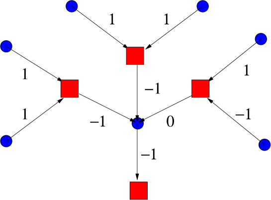
Figure 7: Warning propagation on a factor graph.

Warning Propagation (WP) is an elementary message passing algorithm that uses cavity messages to find a solution of a constraint satisfaction problem. On each edges of the factor graph we define cavity messages $W_{a\rightarrow i}\in\{-1,0,1\},W_{i\rightarrow a}\in\{-1,1\}$; The warning $W_{a\rightarrow i}=0$ means that variable $i$ is free to take any value without worrying about constraint $a$. On the other hand, if $W_{a\rightarrow i}=-1,1$, variable $i$ should take a value that satisfies constraint $a$. The message $W_{i\rightarrow a}=-1,1$ represents the color that variable $i$ has to take to satisfy the other constraints. Given a factor graph we start with the initially random values of $W$’s and in each sweep of the algorithm we update all the messages, see Fig. 7. For example the messages on edge $(i,a)$ are updated in the following way:

$$W_{a\rightarrow i}=\left\{\begin{array}[]{ll}$-1$&\hbox{if all $W_{j\rightarrow a}$'s are $1$},\\ $1$&\hbox{if all $W_{j\rightarrow a}$'s are $-1$},\\ $0$&\hbox{otherwise},\end{array}\right.$$ (48)

$$W_{i\rightarrow a}=\it{sign}(\sum_{b\in V(i)\setminus a}W_{b\rightarrow i}).$$

If the algorithm converges and no variable receives contradictory warnings we can determine the solution according to the warnings. It has been shown that on tree factor graphs the above algorithm always converges and gives the solutions.

More sophisticated message passing algorithms that work much better than WP are Belief Propagation Decimation (BPD) and Survey Propagation Decimation (SPD) BMZ-rsalgorithm-2005 . In these algorithms one replaces the messages $W_{a\rightarrow i},W_{i\rightarrow a}$ with probabilities that come from single cluster (RS) or multiple cluster (1RSB) approximation. For example, in BPD we have the believes $\mu_{a\rightarrow i},\mu_{i\rightarrow a}$ that are updated according to the BP equations

$$\mu_{i\rightarrow a}(\sigma_{i})=\frac{1}{Z_{i\rightarrow a}}\prod_{b\in V(i)\setminus a}\mu_{b\rightarrow i}(\sigma_{i}),$$ (49)

$$\mu_{b\rightarrow i}(\sigma_{i})=\sum_{\sigma_{\partial b\setminus i}}I_{b}(\sigma_{\partial b})\prod_{j\in V(b)\setminus i}\mu_{j\rightarrow b}(\sigma_{j}).$$

Starting from random initial values for the $\mu$’s we update them to reach a fixed point of the dynamics. After convergence we define the local fields

$$H_{i}\equiv\ln\frac{\mu_{i}(1)}{\mu_{i}(0)},$$ (50)

where

$$\mu_{i}(\sigma_{i})=\frac{1}{Z_{i}}\prod_{b\in V(i)}\mu_{b\rightarrow i}(\sigma_{i}).$$ (51)

Then the most biased variable is fixed according to the sign of its local field. Then we simplify the factor graph and repeat the above procedure till we obtain a paramagnet where $H_{i}=0$ for all the remained variables. At this stage we can run a local search algorithm to complete the solution of our problem. In this paper we are going to use a smoothed version of BPD first introduced in BZ-prl-2006 . The main idea is to introduce external fields $h_{i}$ that at each step of the algorithm are updated according to the local fields. At the end, the external fields determine the preferred values of the variables. We call this algorithm Belief Propagation Reinforcement BKMZ-isit-2007 .

More precisely, the BP Reinforcement algorithm works as follows:

• Start with random initial values for $0\leq\mu_{i\rightarrow a},\mu_{a\rightarrow i}\leq 1$ and $-\delta\leq h_{i}\leq\delta$ ($\delta\ll 1$).

• For $t=1,\ldots,t_{max}$ :

  • Update all the $\mu$’s according to the BP equations in presence of the external fields:

    $$\mu_{i\rightarrow a}(\sigma_{i})=\frac{e^{h_{i}\sigma_{i}}}{Z_{i\rightarrow a}}\prod_{b\in V(i)\setminus a}\mu_{b\rightarrow i}(\sigma_{i}),$$ (52)

    $$\mu_{b\rightarrow i}(\sigma_{i})=\sum_{\sigma_{\partial b\setminus i}}I_{b}(\sigma_{\partial b})\prod_{j\in V(b)\setminus i}\mu_{j\rightarrow b}(\sigma_{j}).$$

  • Obtain local fields $H_{i}=\ln\frac{\mu_{i}(1)}{\mu_{i}(0)}$ and with probability $1-t^{-\gamma}$ update the external fields as $h_{i}\rightarrow h_{i}+\it{sign}(H_{i})\delta$.

  • If $\underline{\sigma}=\{\sigma_{i}=\it{sign}(H_{i})|i=1,\ldots,N\}$ is a solution, return SOLUTION $=\underline{\sigma}$.

Notice that instead of fixing variables one by one, here all the external fields are updated (with a rate that increases with $t$) during the run time. Moreover, in this algorithm we do not need to simplify the factor graph after each decimation.

For comparison, we also use other algorithms like Simulated Annealing (SA) and Focused Simulated Annealing (FSA) to find solutions SAO-jstat-2005 . In the SA algorithm we start from a random configuration at small inverse temperature $\beta_{i}\equiv 1/T_{i}$ and decrease the temperature slowly. At each temperature we select all the variables in a random sequential way and flip a variable with probability $\textit{min}\{1,\exp(-\beta\Delta E_{i})\}$. Here $\Delta E_{i}$ is the change in the number of unsatisfied constraints, if we accept to flip variable $i$. After a sweep the inverse temperature increases by $\Delta\beta$. In the FSA algorithm we do the same as SA except that to flip a variable we only select those that belong to unsatisfied constraints.

To check the algorithms and their solutions we consider two different cases; (a) $(4,19)$-hypergraphs ($L_{d}<L<L_{s}$), just after the dynamical transition and before the SAT/UNSAT transition where the thermodynamically relevant clusters are unfrozen. (b) $(6,121)$-hypergraphs ($L_{r}<L<L_{f}$), where the thermodynamically relevant clusters are frozen but still there are some unfrozen clusters.

In case (a) we are able to find some solutions with all BPR, SA and FSA algorithms in a reasonable time. On a $(4,19)$-hypergraph of $N=10^{4}$ variables it takes about $20$ hours for SA and FSA algorithms to find a solution whereas BPR algorithm does the job in about $10$ minutes. In SA and FSA algorithms the parameters are $\beta_{i}=0.1$ and $\Delta\beta=10^{-5}$. In BPR algorithm we used $\gamma=0.05$ and $\delta=0.01$. With these parameters we could obtain a solution at the end of almost all runs.

In case (b) we could only find solutions with the BPR algorithm . Both SA and FSA algorithms were not able to give a solution in a couple of days even for $N=10^{3}$. However, on a hypergraph of size $N=10002$, the BPR algorithm still returns a solution for every instance after a few hours in about $20$ percent of the runs starting with different initial conditions.

We expect the performance of the algorithm could be improved by further optimization. We did not pursue this line as we are interested in a proof of concept rather than in optimizing algorithms over academic benchmarks.

VII.2 Entropy versus distance from a solution

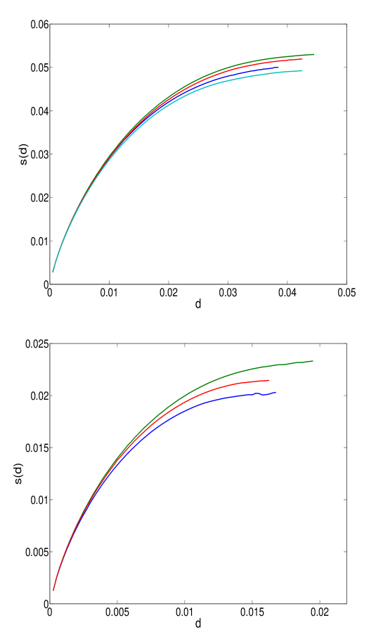
Figure 8: $s(d)$ for a few solutions in a $(4,19)$-hypergraph with $N=10000$ (top) and a $(6,121)$-hypergraph with $N=10002$ (bottom). Please note that some of the curves have been selected to show the extremal behavior of $s(d)$.

Suppose that we have the number of solutions at distance $d$ from a given solution, $e^{Ns(d)}$. If the solution belongs to a sphere-like cluster of solutions then $s(d)$ increases for $d\leq d^{*}$ and becomes zero at $d^{*}$. Clearly, for large $N$, the entropy $s^{*}$ is a good (under)estimate of the total entropy of the cluster. If the solution space is more complex we still expect $s(d)$ to be, up to a distance $d^{*}$, an increasing function of $d$. It may exhibit a maximum at $d^{*}$ and decrease for larger distances. In any case we can take $s^{*}$ as an approximation to the entropy of the cluster.

To obtain $s(d)$ for a given solution $\underline{\sigma}^{*}$ and distance $d$, we use a local BP as follows:

• Start with random initial values for $0\leq\mu_{i\rightarrow a},\mu_{a\rightarrow i}\leq 1$ and a reasonable value of $x$.

• For $t=1,\ldots,t_{max}$ :

  • Update all the $\mu$’s according to the BP equations around the given solution:

    $$\mu_{i\rightarrow a}(\sigma_{i})=\frac{e^{x(\sigma_{i}-\sigma_{i}^{*})^{2}}}{Z_{i\rightarrow a}}\prod_{b\in V(i)\setminus a}\mu_{b\rightarrow i}(\sigma_{i}),$$ (53)

    $$\mu_{b\rightarrow i}(\sigma_{i})=\sum_{\sigma_{\partial b\setminus i}}I_{b}(\sigma_{\partial b})\prod_{j\in V(b)\setminus i}\mu_{j\rightarrow b}(\sigma_{j}).$$

  • Obtain $f(x)$ (Eq. 13) and find the new $x$ such that $d=\frac{\partial f(x)}{\partial x}$.

  • If converged, calculate the entropy (Eq. 15) and return $s(d)$.

The SP version of this algorithm has been used in MM-jstatmech-2006 to obtain the complexity as a function of distance from a solution in $k$-XOR-SAT problem.

Figure 8 shows $s(d)$ for a number of solutions obtained with BPR algorithm. As the figures show, we do not always reach the extrema point of the curve $s(d)$. It is even more difficult to observe the decreasing part of the entropy. Indeed, as we approach the maximum, the convergence time of the algorithm increases rapidly and exceeds the upper bound $t_{max}=1000$. This happens, probably, when we encounter the other clusters where replica symmetry approximation is not valid any more. However, we could observe the decreasing part of $s(d)$ for small values of $N$, where computational time is not too large.

Finally, notice that one could obtain the cluster entropy by summing over all solutions: $\exp(Ns)=\sum_{d}\exp(Ns(d))$. However, for large $N$ the maximum entropy has the dominant contribution to the cluster entropy. To show this we calculated the cluster entropy $s$, using the above definition, and compared it with our estimation $s^{*}$ which is the maximum entropy. For instance, for three solutions of a $(4,19)$-hypergraph of size $N=10000$ we obtain $\delta s=s-s^{*}=0.000115,0.000118,0.000121$ whereas $s^{*}=0.052,0.050,0.0497$, respectively. We see that the differences are very small compared to the cluster entropy.

Another source of systematic error is that the curves do not always reach the real extremum. However, as figure 8 shows, we observed that the maximum entropy is very close to the real one. Indeed an extrapolation of the curves to higher distances gives a correction which is about $0.001$.

VII.3 $m=1$ vs $m\neq 1$ solutions

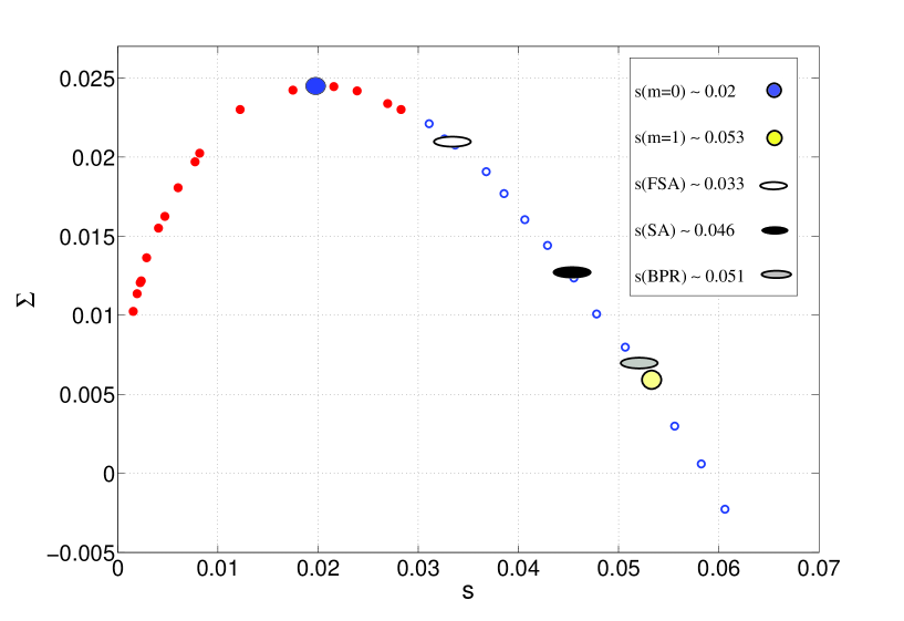
Figure 9: Comparing the attractive clusters of different algorithms in the entropy landscape. The large circles show the typical and thermodynamically relevant clusters. All FSA, SA and BPR algorithms find solutions in the interval between frozen and thermodynamically relevant clusters with entropies $s(FSA)<s(SA)<s(BPR)$. In each case we found $20$ solutions on a $(4,19)$-hypergraph of size $N=10000$. The standard deviations in the entropies is about $0.002$

Using the method described in the previous subsection we can now locate our solutions in the entropy landscape to see to which clusters they belong. In Fig. 9 we show the attractive clusters of different algorithms after the dynamical transition and before the rigidity transition. In this case BPR finds solutions in clusters that are very close to the thermodynamically relevant ones. We think that the difference is due to the systematic errors in underestimating the cluster entropy. In addition, there is also some statistical error in the entropy value of the curve points. The figure also shows that SA ends up in smaller clusters compared to the thermodynamically relevant ones. Moreover, FSA finds solutions in much smaller clusters close to the frozen ones.

The above results have been obtained with parameters given in section VII.1. We found that by decreasing $\gamma$ (in BPR) or $\Delta\beta$ (in SA and FSA) the algorithms find solutions in larger clusters. In fact in a very slow annealing scheme, where one equilibrates the system at each step of the algorithm, we will finally find a solution in the thermodynamically relevant clusters.

Notice that all the algorithms end up in the region between the frozen and thermodynamically relevant clusters. Indeed, when $N$ is large it is very difficult to find a solution in the frozen clusters; each time we flip a frozen variable we go to another cluster of solutions and so an extensive number of flips is needed to accordingly rearrange the variables. On the other hand, it is not also easy to find a solution in very large clusters that are exponentially less numerous than the thermodynamically relevant ones.

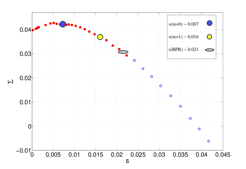
Figure 10: Comparing the attractive clusters of the BPR algorithm with the typical and thermodynamically relevant clusters (large circles). In this case the BPR algorithm finds solutions in the most numerous unfrozen clusters. The result obtained from $20$ solutions on a $(6,121)$-hypergraph of size $N=10002$. The standard deviation in the entropy is about $0.002$.

As already mentioned, beyond the rigidity transition we could only find a solution by BPR algorithm. Figure 10 shows that in this case the solutions are very close to the boundary between frozen and unfrozen clusters. The difference is about the statistical errors and the error that we make by underestimating the entropy. We see that when the thermodynamically relevant clusters are frozen the algorithm ends up in the smallest unfrozen clusters. These are exponentially more numerous than the other unfrozen clusters.

We have checked that our solutions do, indeed, belong to the unfrozen clusters. This can be done with the so called Whitening process P-arxiv-2002 ; AR-proceeding-2006 . Given a solution one checks if a variable can be flipped without violating any constraint. If so, that variable is unfrozen and is denoted with ’$*$’. The process goes on by checking one by one the other variables with the additional rule that a constraint with at least one star variable is always satisfied. This process is repeated up to the fixed point where the number of star variables is fixed. If a solution belongs to an unfrozen cluster then at the end all the variables would be ’$*$’.

VIII Conclusion

In summary we applied the large deviations cavity method to study the phase diagram of the bicoloring problem on regular random hypergraphs. Working in the one-step replica symmetry breaking framework we located the various phase transitions characterizing the structure of the solutions landscape at both the ensemble and single instance level. Notice that we did not check the stability of 1RSB solutions toward higher order replica symmetry breaking. But, as other studies show MR-epjb-2003 ; MPR-jphysa-2004 , we expect 1RSB solutions to give the correct qualitative picture and even exact results close to the SAT/UNSAT transition.

We also used different algorithms to find solutions and to locate them in the entropy landscape of the problem. This provided a rough characterization of the relations existing between the entropic properties of clusters of solutions and the different algorithms used to find them.

From an algorithmic point of view, the algorithms based on simulated annealing could not efficiently find solutions after the rigidity point. However, using BPR we showed that it is actually possible to go beyond the rigidity transition. In this case we obtained solutions that belong to the smallest and most numerous unfrozen clusters S-arxiv-2007 .

Appendix A Cavity equations in the RS approximations

We start from the partition function definition in Eq. 9 and derive the main equations in the first part of section IV. Let $Z_{i\rightarrow a}(\sigma_{i})$ denote the partition function in the absence of constraint $a$ and when variable $i$ has state $\sigma_{i}$. Then, in the absence of constraint $a$, the probability of finding variable $i$ in state $\sigma_{i}$ is

$$\mu_{i\rightarrow a}(\sigma_{i})=\frac{Z_{i\rightarrow a}(\sigma_{i})}{\sum_{\sigma}Z_{i\rightarrow a}(\sigma)}.$$ (A-1)

On the other hand, assuming a tree structure for the factor graph we can write

$$Z_{i\rightarrow a}(\sigma_{i})=\sum_{\sigma_{\partial i\rightarrow a}}\left(\prod_{b\in V(i)\setminus a}I_{b}(\sigma_{\partial b})[\prod_{j\in V(b)\setminus i}Z_{j\rightarrow b}(\sigma_{j})]\right)e^{x(\sigma_{i}-\sigma_{i}^{*})^{2}}.$$ (A-2)

From the above equation we can derive a relation for the cavity marginals

$$\mu_{i\rightarrow a}(\sigma_{i})=\frac{1}{Z_{i\rightarrow a}}\sum_{\sigma_{\partial i\rightarrow a}}\left(\prod_{b\in V(i)\setminus a}I_{b}(\sigma_{\partial b})[\prod_{j\in V(b)\setminus i}\mu_{j\rightarrow b}(\sigma_{j})]\right)e^{x(\sigma_{i}-\sigma_{i}^{*})^{2}},$$ (A-3)

where $Z_{i\rightarrow a}$ is a normalization constant. It is more convenient if we write the above relation as

$$\mu_{i\rightarrow a}(\sigma_{i})=\frac{e^{x(\sigma_{i}-\sigma_{i}^{*})^{2}}}{Z_{i\rightarrow a}}\prod_{b\in V(i)\setminus a}\mu_{b\rightarrow i}(\sigma_{i}),$$ (A-4)

where

$$\mu_{b\rightarrow i}(\sigma_{i})=\sum_{\sigma_{\partial b\setminus i}}I_{b}(\sigma_{\partial b})\prod_{j\in V(b)\setminus i}\mu_{j\rightarrow b}(\sigma_{j}).$$ (A-5)

The free energy $f(x)$ is given by $\frac{1}{N}\ln Z$. In the Bethe approximation

$$f(x)=\sum_{i}\Delta f_{i}-\sum_{a}(K_{a}-1)\Delta f_{a},$$ (A-6)

where $\Delta f_{i}$ and $\Delta f_{a}$ are the free energy shifts by adding variable node $i$ and function node $a$, respectively.

Suppose that we have removed node $i$ and all its function nodes from the factor graph. In this case the partition function reads

$$Z_{-\{i,V(i)\}}=\prod_{a\in V(i)}[\prod_{j\in V(a)\setminus i}Z_{j\rightarrow a}],$$ (A-7)

whereas in the complete factor graph

$$Z=\sum_{\sigma_{i},\sigma_{\partial i}}\prod_{a\in V(i)}[I_{a}(\sigma_{\partial a})\prod_{j\in V(a)\setminus i}Z_{j\rightarrow a}(\sigma_{j})]e^{x(\sigma_{i}-\sigma_{i}^{*})^{2}}.$$ (A-8)

Dividing the two quantities we get

$$\frac{Z}{Z_{-\{i,V(i)\}}}=e^{N\Delta f_{i}}=\sum_{\sigma_{i},\sigma_{\partial i}}\prod_{a\in V(i)}[I_{a}(\sigma_{\partial a})\prod_{j\in V(a)\setminus i}\frac{Z_{j\rightarrow a}(\sigma_{j})}{Z_{j\rightarrow a}}]e^{x(\sigma_{i}-\sigma_{i}^{*})^{2}},$$ (A-9)

and this gives the shift in the free energy by adding variable node $i$

$$e^{N\Delta f_{i}}=\sum_{\sigma_{i}}\prod_{a\in V(i)}\mu_{a\rightarrow i}(\sigma_{i})e^{x(\sigma_{i}-\sigma_{i}^{*})^{2}}.$$ (A-10)

We can do the same procedure for a function node. If we remove function node $a$ from the factor graph we have

$$Z_{-a}=\prod_{i\in V(a)}Z_{i\rightarrow a},$$ (A-11)

whereas the complete partition function can be written as

$$Z=\sum_{\sigma_{\partial a}}I_{a}(\sigma_{\partial a})\prod_{i\in V(a)}Z_{i\rightarrow a}(\sigma_{i}).$$ (A-12)

So

$$\frac{Z}{Z_{-a}}=e^{N\Delta f_{a}}=\sum_{\sigma_{\partial a}}I_{a}(\sigma_{\partial a})\prod_{i\in V(a)}\frac{Z_{i\rightarrow a}(\sigma_{i})}{Z_{i\rightarrow a}},$$ (A-13)

and the shift in the free energy is given by

$$e^{N\Delta f_{a}}=\sum_{\sigma_{\partial a}}I_{a}(\sigma_{\partial a})\prod_{i\in V(a)}\mu_{i\rightarrow a}(\sigma_{i}).$$ (A-14)

Finally using Eqs. A-6, A-10 and A-14 we obtain the free energy $f(x)$ in the Bethe approximation

$$Nf(x)=\sum_{i}\ln Z_{i}-\sum_{a}(K_{a}-1)\ln Z_{a},$$ (A-15)

$$Z_{i}\equiv\sum_{\sigma_{i}}[\prod_{a\in V(i)}\mu_{a\rightarrow i}(\sigma_{i})]e^{x(\sigma_{i}-\sigma_{i}^{*})^{2}},$$

$$Z_{a}\equiv\sum_{\sigma_{\partial a}}I_{a}(\sigma_{\partial a})\prod_{i\in V(a)}\mu_{i\rightarrow a}(\sigma_{i}).$$

Appendix B Cavity equations in the 1RSB approximation

We start from the generalized partition function in Eq. 16 and explain the main equations in the second part of section IV.

In the Bethe approximation

$$N\mathcal{F}(m)=\sum_{i}\Delta\mathcal{F}_{i}-\sum_{a}(K_{a}-1)\Delta\mathcal{F}_{a}.$$ (B-16)

The generalized partition function can be written as

$$\mathcal{Z}=\sum_{c}e^{mN[s_{c,-\{i,V(i)\}}+\Delta s_{c,i}]},$$ (B-17)

where $\Delta s_{c,i}$ is the shift in the entropy of cluster $c$ by adding node $i$ and all its function nodes. At a fixed value of $m$ the typical clusters would have nearly the same entropy and it seems safe to approximate $e^{mN\Delta s_{i}}$ with its average value among the clusters, i.e.

$$\mathcal{Z}=[\sum_{c}e^{mNs_{c,-\{i,V(i)\}}}]\int d\mathcal{P}[\mu]e^{mN\Delta s_{i}},$$ (B-18)

where $\mathcal{P}[\mu]$ is the probability distribution of $\mu_{i\rightarrow a}$’s among the clusters. So the shift in the generalized free energy reads

$$e^{N\Delta\mathcal{F}_{i}}=\int\prod_{a\in V(i)}\prod_{j\in V(a)\setminus i}d\mathcal{P}_{j\rightarrow a}[\mu_{j\rightarrow a}]e^{mN\Delta s_{i}}.$$ (B-19)

In the case of adding a function node, similarly we find

$$e^{N\Delta\mathcal{F}_{a}}=\int\prod_{i\in V(a)}d\mathcal{P}_{i\rightarrow a}[\mu_{i\rightarrow a}]e^{mN\Delta s_{a}}.$$ (B-20)

Notice that $\Delta s_{i}$ and $\Delta s_{a}$ correspond to the free energy shifts, Eqs. A-10 and A-14, with $x=0$. Using Eqs. B-19 and B-20 along with the Bethe form of the generalized free energy we obtain

$$N\mathcal{F}(m)=\sum_{i}\ln\mathcal{Z}_{i}-\sum_{a}(K_{a}-1)\ln\mathcal{Z}_{a},$$ (B-21)

$$\mathcal{Z}_{i}\equiv\int D_{i}\mathcal{P}[\mu]e^{mN\Delta s_{i}},$$

$$\mathcal{Z}_{a}\equiv\int D_{a}\mathcal{P}[\mu]e^{mN\Delta s_{a}},$$

where $d\mathcal{P}[\mu]$ is determined by Eq. 20. The normalization constant in this equation is

$$\mathcal{Z}_{i\rightarrow a}=\int\prod_{b\in V(i)\setminus a}\prod_{j\in V(b)\setminus i}d\mathcal{P}_{j\rightarrow b}[\mu]e^{mN\Delta s_{i}}.$$ (B-22)

We represented $\mathcal{P}[\mu]$ as

$$\mathcal{P}[\mu]=\frac{1-\pi}{2}[\delta(r)+\delta(r-1)]+\pi\rho(r),$$ (B-23)

where $\rho(r)$ is the probability distribution of unfrozen marginals. By the normalization and symmetry of the problem

$$\int dr\rho(r)=1,$$ (B-24)

$$\int drr\rho(r)=\int dr(1-r)\rho(r)=\frac{1}{2}.$$

Then for the $\mathcal{Q}_{i\rightarrow a}^{\sigma}[\mu]=2\mu_{i\rightarrow a}(\sigma)\mathcal{P}_{i\rightarrow a}[\mu]$ we have

$$\mathcal{Q}_{i\rightarrow a}^{0}[\mu]=(1-\pi)\delta(1-r)+2\pi r\rho(r),$$ (B-25)

$$\mathcal{Q}_{i\rightarrow a}^{1}[\mu]=(1-\pi)\delta(r)+2\pi(1-r)\rho(r).$$

Notice that for $\sigma\in\{0,1\}$

$$\int d\mu\mathcal{Q}_{i\rightarrow a}^{\sigma}[\mu]=1.$$ (B-26)

Appendix C Calculating the generalized free energy

To calculate the free energy $\mathcal{F}$ we need to obtain $\mathcal{Z}_{i}$, $\mathcal{Z}_{a}$, the fraction of unfrozen variables $\pi$ and $\rho(r)$. Let us start from Eq. 20 and multiply both sides of the equation with $e^{-rt}$. Integrating over $r$ allows us to get rid of delta function and we find

$$\frac{1-\pi}{2}(1+e^{-t})+\pi\int\rho(r)e^{-rt}dr\hskip 85.35826pt$$ (C-27)

$$=\frac{1}{\mathcal{Z}_{i\rightarrow a}}\prod_{b\in V(i)\setminus a}[\sum_{n_{b}^{0},n_{b}^{1},n_{b}^{*}}\left(\begin{array}[]{c}K-1\\ n_{b}^{0},n_{b}^{1},n_{b}^{*}\end{array}\right)(\frac{1-\pi}{2})^{n_{b}^{0}+n_{b}^{1}}\pi^{n_{b}^{*}}\prod_{j\in V^{*}(b)}\int dr_{b}^{j}\rho(r_{b}^{j})]$$ (C-30)

$$\times[\prod_{b}\lambda_{0}(n_{b},r_{b})+\prod_{b}\lambda_{1}(n_{b},r_{b})]^{m}e^{-\frac{t}{Z_{i\rightarrow a}}\prod_{b}\lambda_{0}(n_{b},r_{b})},$$

where $n_{b}^{0}$ and $n_{b}^{1}$ are the number of frozen variables in $V(b)\setminus i$ that take values $0$ and $1$, respectively. Accordingly $V^{*}(b)\setminus i$ is the set of unfrozen variables in $V(b)\setminus i$ and $n_{b}^{*}$ is the number of its elements. Notice that $n_{b}$’s should satisfy $n^{0}+n_{b}^{1}+n_{b}^{*}=K-1$.

Using Eqs. A-3 and A-10 we write

$$r=\frac{1}{Z_{i\rightarrow a}}\prod_{b\in V(i)\setminus a}\lambda_{0}(n_{b},r_{b}),$$ (C-31)

$$e^{N\Delta s_{i}}=\prod_{b\in V(i)}\lambda_{0}(n_{b},r_{b})+\prod_{b\in V(i)}\lambda_{1}(n_{b},r_{b}),$$

where

$$\lambda_{0}(n_{b},r_{b})=(1-\delta_{n_{b}^{0},K-1})[1-\delta_{n_{b}^{1},0}(1-\delta_{n_{b}^{*},0})\prod_{j\in V^{*}(b)\setminus i}r_{b}^{j}],$$ (C-32)

$$\lambda_{1}(n_{b},r_{b})=(1-\delta_{n_{b}^{1},K-1})[1-\delta_{n_{b}^{0},0}(1-\delta_{n_{b}^{*},0})\prod_{j\in V^{*}(b)\setminus i}(1-r_{b}^{j})].$$

One can use Eq. C-27 to write some equations for different moments of $\rho(r)$. For example, for the second moment we obtain

$$\frac{1-\pi}{2}+\pi\langle r^{2}\rangle=\frac{1}{\mathcal{Z}_{i\rightarrow a}}\prod_{b\in V(i)\setminus a}[\sum_{n_{b}^{0},n_{b}^{1},n_{b}^{*}}\left(\begin{array}[]{c}K-1\\ n_{b}^{0},n_{b}^{1},n_{b}^{*}\end{array}\right)(\frac{1-\pi}{2})^{n_{b}^{0}+n_{b}^{1}}\pi^{n_{b}^{*}}$$ (C-35)

$$\times\prod_{j\in V^{*}(b)\setminus i}\int dr_{b}^{j}\rho(r_{b}^{j})][\prod_{b\in V(i)\setminus a}\lambda_{0}(n_{b},r_{b})+\prod_{b\in V(i)\setminus a}\lambda_{1}(n_{b},r_{b})]^{m}(\frac{\prod_{b}\lambda_{0}(n_{b},r_{b})}{Z_{i\rightarrow a}})^{2}.$$

To compute $\mathcal{F}$ we also need to find $e^{N\Delta s_{a}}$ in Eq. A-14

$$e^{N\Delta s_{a}}=(1-\delta_{n_{a}^{0},K})(1-\delta_{n_{a}^{1},K})[1-\delta_{n_{a}^{1},0}(1-\delta_{n_{a}^{*},0})\prod_{i\in V^{*}(a)}r_{a}^{j}-\delta_{n_{a}^{0},0}(1-\delta_{n_{a}^{*},0})\prod_{i\in V^{*}(a)}(1-r_{a}^{i})].$$ (C-36)

The normalization constants in Eqs. A-2 and B-22 are

$$Z_{i\rightarrow a}=\prod_{b\in V(i)\setminus a}\lambda_{0}(n_{b},r_{b})+\prod_{b\in V(i)\setminus a}\lambda_{1}(n_{b},r_{b}),$$ (C-37)

and

$$\mathcal{Z}_{i\rightarrow a}=\prod_{b\in V(i)\setminus a}[\sum_{n_{b}^{0},n_{b}^{1},n_{b}^{*}}\left(\begin{array}[]{c}K-1\\ n_{b}^{0},n_{b}^{1},n_{b}^{*}\end{array}\right)(\frac{1-\pi}{2})^{n_{b}^{0}+n_{b}^{1}}\pi^{n_{b}^{*}}\prod_{j\in V^{*}(b)\setminus i}\int dr_{b}^{j}\rho(r_{b}^{j})]$$ (C-40)

$$\times[\prod_{b\in V(i)\setminus a}\lambda_{0}(n_{b},r_{b})+\prod_{b\in V(i)\setminus a}\lambda_{1}(n_{b},r_{b})]^{m}.$$

Finally for the main elements of the generalized free energy we have

$$\mathcal{Z}_{i}=\prod_{b\in V(i)}[\sum_{n_{b}^{0},n_{b}^{1},n_{b}^{*}}\left(\begin{array}[]{c}K-1\\ n_{b}^{0},n_{b}^{1},n_{b}^{*}\end{array}\right)(\frac{1-\pi}{2})^{n_{b}^{0}+n_{b}^{1}}\pi^{n_{b}^{*}}\prod_{j\in V^{*}(b)\setminus i}\int dr_{b}^{j}\rho(r_{b}^{j})]$$ (C-43)

$$\times[\prod_{b\in V(i)\setminus a}\lambda_{0}(n_{b},r_{b})+\prod_{b\in V(i)\setminus a}\lambda_{1}(n_{b},r_{b})]^{m},$$

and

$$\mathcal{Z}_{a}=\sum_{n_{a}^{0},n_{a}^{1},n_{a}^{*}}\left(\begin{array}[]{c}K\\ n_{a}^{0},n_{a}^{1},n_{a}^{*}\end{array}\right)(\frac{1-\pi}{2})^{n_{a}^{0}+n_{a}^{1}}\pi^{n_{a}^{*}}\prod_{i\in V^{*}(a)}\int dr_{a}^{i}\rho(r_{a}^{i})[(1-\delta_{n_{a}^{0},K})(1-\delta_{n_{a}^{1},K})$$ (C-46)

$$\times\left(1-\delta_{n_{a}^{1},0}(1-\delta_{n_{a}^{*},0})\prod_{i\in V^{*}(a)}r_{a}^{j}-\delta_{n_{a}^{0},0}(1-\delta_{n_{a}^{*},0})\prod_{i\in V^{*}(a)}(1-r_{a}^{i})\right)]^{m}.$$

In the following we will give the details of calculations in two special cases that need more explanation.

C.1 The case $\pi=1$

When $\pi=1$ the equation for $\mathcal{Z}_{i}$, Eq. C-43, is

$$\mathcal{Z}_{i}=\prod_{a=1,L}[\prod_{j=1,K-1}\int dr_{a}^{j}\rho(r_{a}^{j})][\prod_{a}\left(1-\prod_{j}r_{a}^{j}\right)+\prod_{a}\left(1-\prod_{j}(1-r_{a}^{j})\right)]^{m}.$$ (C-47)

For $m=0,1,2$ we obtain

$$\mathcal{Z}_{i}(m=0)=1,\hskip 85.35826pt$$ (C-48)

$$\mathcal{Z}_{i}(m=1)=2[1-\frac{1}{2^{K-1}}]^{L},\hskip 85.35826pt$$

$$\mathcal{Z}_{i}(m=2)=2[1-\frac{2}{2^{K-1}}+\langle r^{2}\rangle^{K-1}]^{L}+2[1-\frac{2}{2^{K-1}}+(\frac{1}{2}-\langle r^{2}\rangle)^{K-1}]^{L}.$$

For $\mathcal{Z}_{a}$ from Eq. C-46 we find

$$\mathcal{Z}_{a}=[\prod_{i=1,K}\int dr_{a}^{i}\rho(r_{a}^{i})][1-\prod_{i}r_{a}^{i}-\prod_{i}(1-r_{a}^{i})]^{m}.$$ (C-49)

Again for $m=0,1,2$

$$\mathcal{Z}_{a}(m=0)=1,$$ (C-50)

$$\mathcal{Z}_{a}(m=1)=[1-\frac{2}{2^{K}}],$$

$$\mathcal{Z}_{a}(m=2)=[1-\frac{4}{2^{K}}+2\langle r^{2}\rangle^{K}+2(\frac{1}{2}-\langle r^{2}\rangle)^{K}].$$

To complete the free energy calculations we need to find $\langle r^{2}\rangle$ in $m=2$ clusters. The second moment of $\rho(r)$ can be obtained from Eq. C-35,

$$\langle r^{2}\rangle=\frac{1}{\mathcal{Z}_{i\rightarrow a}}\prod_{b=1,L-1}[\prod_{j=1,K-1}\int dr_{b}^{j}\rho(r_{b}^{j})]\hskip 56.9055pt$$ (C-51)

$$\times[\prod_{b}\left(1-\prod_{j}r_{b}^{j}\right)+\prod_{b}\left(1-\prod_{j}(1-r_{b}^{j})\right)]^{m-2}[\prod_{b}\left(1-\prod_{j}r_{b}^{j}\right)]^{2}.$$

If $m=2$, the exact equation is

$$\langle r^{2}\rangle=\frac{1}{\mathcal{Z}_{i\rightarrow a}(m=2)}[1-\frac{2}{2^{K-1}}+\langle r^{2}\rangle^{K-1}]^{L-1}.$$ (C-52)

Now we can use the Lagrange interpolating polynomial to approximate the free energy by

$$\mathcal{F}(m)=\mathcal{F}(m=0)\frac{(m-1)(m-2)}{2}-\mathcal{F}(m=1)m(m-2)+\mathcal{F}(m=2)\frac{m(m-1)}{2}.$$ (C-53)

Since $\mathcal{F}(m=0)=0$ we get

$$\mathcal{F}(m)=-\mathcal{F}(m=1)m(m-2)+\mathcal{F}(m=2)\frac{m(m-1)}{2},$$ (C-54)

$$s(m)=-2(m-1)\mathcal{F}(m=1)+(m-\frac{1}{2})\mathcal{F}(m=2),$$

$$\Sigma(m)=m^{2}[\mathcal{F}(m=1)-\frac{1}{2}\mathcal{F}(m=2)].$$

C.2 The case of integer $m$

Starting from Eq. B-22 we expand $\mathcal{Z}_{i\rightarrow a}$ for integer $m>0$ to get

$$\mathcal{Z}_{i\rightarrow a}=\sum_{l}\left(\begin{array}[]{c}m\\ l\end{array}\right)\prod_{b\in V(i)\setminus a}[\sum_{n_{b}^{0},n_{b}^{1},n_{b}^{*}}\left(\begin{array}[]{c}K-1\\ n_{b}^{0},n_{b}^{1},n_{b}^{*}\end{array}\right)(\frac{1-\pi}{2})^{n_{b}^{0}+n_{b}^{1}}\pi^{n_{b}^{*}}$$ (C-59)

$$\times\prod_{j\in V^{*}(b)}\int dr_{b}^{j}\rho(r_{b}^{j})\lambda_{0}^{l}(n_{b},r_{b})\lambda_{1}^{m-l}(n_{b},r_{b})].$$

To simplify the results we approximate $\rho(r)$ by $\delta(r-\frac{1}{2})$. After some simplifications we obtain

$$\mathcal{Z}_{i\rightarrow a}=\sum_{l}\left(\begin{array}[]{c}m\\ l\end{array}\right)[1-2(\frac{1+\pi}{2})^{K-1}+\pi^{K-1}+\pi^{K-1}(1-\frac{1}{2^{K-1}})^{m}$$ (C-62)

$$-\pi^{K-1}(1-\frac{1}{2^{K-1}})^{l}-\pi^{K-1}(1-\frac{1}{2^{K-1}})^{m-l}$$

$$+\sum_{n}\left(\begin{array}[]{c}K-1\\ n\end{array}\right)(\frac{1-\pi}{2})^{K-1-n}\pi^{n}\left((1-\frac{1}{2^{n}})^{l}+(1-\frac{1}{2^{n}})^{m-l}\right)]^{L-1}.$$ (C-65)

For $\mathcal{Z}_{a}$ we use Eq. C-46 and again $\rho(r)=\delta(r-\frac{1}{2})$ to get

$$\mathcal{Z}_{a}=\pi^{K}[1-\frac{2}{2^{K}}]^{m}-2\pi^{K}[1-\frac{1}{2^{K}}]^{m}\hskip 56.9055pt$$ (C-66)

$$+2\sum_{n}\left(\begin{array}[]{c}K\\ n\end{array}\right)(\frac{1-\pi}{2})^{K-n}\pi^{n}[1-\frac{1}{2^{n}}]^{m}+[1+\pi^{K}-2(\frac{1+\pi}{2})^{K}].$$ (C-69)

To obtain the free energy we still need to determine $\pi$. From Eq. 21 we have

$$1-\pi=\frac{2^{-(K-1)(L-1)+1}}{\mathcal{Z}_{i\rightarrow a}}\sum_{l=1,L-1}\left(\begin{array}[]{c}L-1\\ l\end{array}\right)[(1-\pi)^{K-1}]^{l}\hskip 56.9055pt$$ (C-72)

$$\times[\sum_{\sigma_{\partial b\setminus i}}I_{b}(\sigma_{\partial b\setminus i})\int\prod_{j\in V(b)\setminus i}d\mathcal{Q}^{\sigma_{j}}[\mu]\left(1-\delta_{n_{b}^{1},0}(1-\delta_{n_{b}^{*},0})\prod_{j\in V(b)\setminus i}r_{b}^{j}\right)^{m-1}]^{L-1-l}.$$

Taking $\rho(r)=\delta(r-\frac{1}{2})$ we obtain an equation for $\pi$ and for general $m$.

$$\frac{1-\pi}{2}\hskip 369.88582pt$$ (C-73)

$$=\frac{1}{\mathcal{Z}_{i\rightarrow a}}\{[1-(\frac{1+\pi}{2})^{K-1}+\sum_{n}\left(\begin{array}[]{c}K-1\\ n\end{array}\right)(\frac{1-\pi}{2})^{K-1-n}\pi^{n}(1-\frac{1}{2^{n}})^{m}]^{L-1}$$ (C-76)

$$-[1-(\frac{1+\pi}{2})^{K-1}-(\frac{1-\pi}{2})^{K-1}+\sum_{n}\left(\begin{array}[]{c}K-1\\ n\end{array}\right)(\frac{1-\pi}{2})^{K-1-n}\pi^{n}(1-\frac{1}{2^{n}})^{m}]^{L-1}\}.$$ (C-79)

References

• (1) R. G. Gallager, Information Theory and Reliable Communication. Wiley, New York, 1968.
• (2) D. J. C. MacKay, Information Theory, Inference and Learning Algorithms. Cambridge University Press, Cambridge, 2002.
• (3) Special Issue on NP-hardness and Phase transitions, edited by O. Dubois, R. Monasson, B. Selman and R. Zecchina, Theor. Comp. Sci. 265, Issue: 1-2 (2001).
• (4) D. Challet, M. Marsili and R. Zecchina, Phys. Rev. Lett. 84, 1824 (2000).
• (5) T. Galla, M. Leone, M. Marsili, M. Sellitto, M. Weigt and R. Zecchina, Phys. Rev. Lett. 97, 128701 (2006)
• (6) A. Braunstein and R. Zecchina, Phys. Rev. Lett. 96, 030201 (2006).
• (7) C. Baldassi, A. Braunstein, N. Brunel and R. Zecchina, PNAS 104(26), 11079 (2007).
• (8) S. Cook. The complexity of theorem proving procedures. In Proceedings of the Third Annual ACM Symposium on Theory of Computing, pages 151-158, 1971.
• (9) M. Garey and D. Johnson, Computers and Intractability – A Guide to the Theory of NP-completeness, Freeman (1979).
• (10) S. Kirkpatrick, B. Selman, Science 264, 1297 (1994).
• (11) R. Monasson, R. Zecchina, S. Kirkpatrick, B. Selman, and L. Troyanski, Nature 400, 133 (1999).
• (12) M. Mézard, F. Ricci-Tersenghi, R. Zecchina, J. Stat. Phys. 111, 505 (2003).
• (13) S. Cocco, O. Dubois, J. Mandler, R. Monasson, Phys. Rev. Lett. 90, 047205 (2003).
• (14) M. Mézard, M. Palassini and O. Rivoire, Phys. Rev. Lett. 95, 200202 (2005).
• (15) T. Mora, PhD Thesis (2007).
• (16) F. Krzakala, A. Montanari, F. Ricci-Tersenghi, G. Semerjian and L. Zdeborova, PNAS 104(25), 10318 (2007).
• (17) L. Zdeborova and F. Krzakala, Phys. Rev. E, 76 (3), 031131 (2007).
• (18) G. Semerjian, J. Stat. Phys. 130, 251 (2008).
• (19) F. Krzakala and J. Kurchan, Phys. Rev. E, 76 (2), 021122 (2007).
• (20) R. Monasson, R. Zecchina, Phys. Rev. E 56, 1357 (1997).
• (21) M. Mézard, G. Parisi and R. Zecchina, Science 297, 812 (2002).
• (22) M. Mézard and R. Zecchina, Phys. Rev. E 66, 056126 (2002).
• (23) R. Mulet, A. Pagnani, M. Weigt and R. Zecchina, Phys. Rev. Lett. 89, 268701 (2002).
• (24) D. Achlioptas, A. Naor and Y. Peres, Nature 435, 759 (2005).
• (25) S. Mertens, M. Mézard, R. Zecchina, Random Structure and Algorithms 28, 340 (2006).
• (26) M. Mezard, G. Parisi and M. A. Virasoro, Spin-Glass Theory and Beyond, vol 9 of Lecture Notes in Physics (World Scientific, Singapore, 1987).
• (27) M. Mézard, G. Parisi, Eur. Phys. J. B 20, 217 (2001).
• (28) M. Mézard, G. Parisi, J. Stat. Phys. 111 (1-2), 1 (2003).
• (29) O. Rivoire, J. Stat. Mech. P07004 (2005)
• (30) F. R. Kschischang, B. J. Frey and H. -A. Loeliger, IEEE Trans. Infor. Theory 47, 498 (2001)
• (31) E. Friedgut, J. Amer. Math. Soc. 12, 1017 (1999).
• (32) T. Castellani, V. Napolano, F. Ricci-Tersenghi and R. Zecchina, J. Phys. A: Math. Gen 36, 11037 (2003).
• (33) A. Braunstein, M. Mezard and R. Zecchina, Random Structures Algorithms 27, 201 (2005).
• (34) A. Braunstein, F. Kahyan, G. Montorsi, R. Zecchina, proceedings of the IEEE Int. Symposium of Information Theory ISIT 2007, arXiv:0705.0423.
• (35) S. Seitz, M. Alava and P. Orponen, J. Stat. Mech. (2005) P06006.
• (36) T. Mora, M. Mézard, J. Stat. Mech. P10007 (2006).
• (37) G. Parisi, cs.CC/0212047.
• (38) D. Achlioptas and F. Ricci-Tersenghi, Proceedings of the 38th Annual ACM Symposium on Theory of Computing, Session 4A, 130 (2006).
• (39) A. Montanari and F. Ricci-Tersenghi, Eur. Phys. J B 33, 339 (2003).
• (40) A. Montanari, G. Parisi and F. Ricci-Tersenghi, J. Phys. A: Math. Gen. 37, 2073 (2004).