Ellipsoidal particles at fluid interfaces
Abstract
For partially wetting, ellipsoidal colloids trapped at a fluid interface, their effective, interface–mediated interactions of capillary and fluctuation–induced type are analyzed. For contact angles different from 90o, static interface deformations arise which lead to anisotropic capillary forces that are substantial already for micrometer–sized particles. The capillary problem is solved using an efficient perturbative treatment which allows a fast determination of the capillary interaction for all distances between and orientations of two particles. Besides static capillary forces, fluctuation–induced forces caused by thermally excited capillary waves arise at fluid interfaces. For the specific choice of a spatially fixed three–phase contact line, the asymptotic behavior of the fluctuation–induced force is determined analytically for both the close–distance and the long–distance regime and compared to numerical solutions.
pacs:
82.70.DdColloids and 68.03.Cd Surface tension and related phenomena and 05.40.-aFluctuation phenomena, random processes, noise, and Brownian motion1 Introduction
Colloidal particles trapped at fluid interfaces exhibit effective interactions which broadly can be classified into “direct” interactions (e.g., of electrostatic or van–der–Waals type) which also exist for colloids in bulk solvents but they are modified at interfaces. Additionally, the presence of an interface gives rise to interactions mediated by deformations of that interface, thus these are absent in bulk solutions of colloids. One speaks of capillary interactions Kra00 , if these deformations are static, and of fluctuation–induced interactions if the deformations are caused by thermal fluctuations. For spherical colloids at free interfaces, the formation of self–organized structures is mainly governed by the direct interactions whereas for particles of nonspherical shape capillary interactions appear to be dominant Bre07r .
Static interface deformations arise if the colloids experience forces in the direction parallel to the interface normal (e.g. if they are pushed into the lower phase) and/or stress distributions act on the interface Oet08 . For microcolloids of sizes less than 10 m, the omnipresent gravitational force on the colloids can be neglected. However, meniscus deformations also arise in conjunction with direct interactions (like electrostatic forces) which lead to forces and stresses on colloids and interface, respectively. If the system “colloids + interface” is mechanically isolated (usually this applies for colloid experiments in a Langmuir trough or on large droplets), then the force on the colloids directed vertical to the interface is balanced by the total force on the interface (obtained by integrating the stress distribution over the interface area) For04 ; Dom05 ; Dom07 . The ensuing capillary interactions decay with a power–law in the intercolloidal distance , e.g., in the case of charged colloidal spheres at air–water or oil–water interfaces they are attractive, , but for large they are usually weaker than the direct electrostatic repulsion which is also Oet05a ; Wue05 ; Fry07 . – On the other hand, in the absence of forces on the colloids and stresses on the interface, static interface deformations can also be induced by an anisotropic colloid shape; more precisely if the colloid is not symmetric with respect to rotations around any axis through the colloid which is parallel to the normal on the undisturbed interface. Young’s equation requires that at the three–phase contact line the angle between the local interface normal and the local normal on the colloid surface is given by the contact angle . Thus for an anisotropic colloid this condition cannot be met if the interface remains flat; the contact line will not be located in the plane of the undisturbed interface. The associated interface deformations around one such colloid can be calculated in terms of a two–dimensional multipolar expansion Fou02 . For asymptotically large distances from the colloid, the leading nonvanishing multipole is in general the quadrupole, since monopole and dipole are absent through the conditions of force and torque balance. The interaction energy between two quadrupoles depends on the colloid orientation in the interface plane and decays according to a power law, . Experimentally, it has become possible to produce anisotropic microcolloids of controlled shape for investigations of their self–assembly at fluid interfaces: anorganic nanorods Yan02 , bended disks Ren01 or rotationally symmetric ellipsoids (spheroids) with aspect ratios up to 10 Lou05 ; Bas06 . For the ellipsoids, results on the effective pair potential for intermediate distances Lou05 indicate a strong orientation dependence not captured by the aformentioned leading quadrupole interaction. Ellipsometric measurements of the interface deformation around one particle are consistent with a quadrupolar pattern Lou06 which, however, appears to be deformed considerably for stretched ellipsoids.
The calculation of the full interface profile around trapped ellipsoids and the evaluation of the associated capillary interaction energy can only be done numerically, save for small eccentricities where an expansion in terms of is possible Nie05 . Similarly, an evaluation of the interface profile is simplified if for colloidal spheres only small, roughness–induced deviations from the circular shape of the contact line are assumed Sta00 ; Dan05 . For ellipsoids with eccentricities not close to zero, however, the position of the contact line is not given a priori but has to be determined self–consistently through Young’s equation. This task is a variant of a free boundary problem which in general poses problems in terms of speed and efficiency of a numerical algorithm aimed at solving it. Below, we show that a perturbative solution can be attained through expansion of an appropriate free energy functional and subsequent minimization which leads to a problem with fixed boundaries (Subsec. 2.1). The calculation of the capillary interaction between two ellipsoids is thus greatly simplified and results can be obtained for the full range of distances and orientations in a configuration with two ellipsoids (Subsec. 2.2).
The capillary interactions between two ellipsoids are absent if the contact angle equals , and they become significantly smaller for ellipsoid sizes approaching the molecular length scale. In these circumstances, fluctuations around the equilibrium interface position are expected to influence the effective interactions noticeably. Since the interface fluctuations are of thermal nature, the scale of the ensuing interactions will be given by , the thermal energy. Within a coarse–grained picture, the properties of fluid interfaces are very well described by an effective capillary wave Hamiltonian which governs both the equilibrium interface configuration and the thermal fluctuations (capillary waves) around this equilibrium (or mean-field) position. As postulated by the Goldstone theorem the capillary waves are long-range correlated. The interface breaks the continuous translational symmetry of the system, and in the limit of vanishing external fields – like gravity – it has to be accompanied by easily excitable long wavelength (Goldstone) modes – precisely the capillary waves. The fluctuation spectrum of the capillary waves will be modified by colloids trapped at the interface and therefore leads to fluctuation–induced forces between them. In that respect, colloids at fluids interfaces appear to be a possible realization of a two–dimensional system exhibiting the Casimir effect. For spheres and disks, these forces have been calculated in Refs. Leh06 ; Leh07b . The large–distance behavior of these forces depends sensitively on the boundary conditions at the three–phase contact line whereas for close distances a strong attraction similar to van–der–Waals forces has been found, independent of the type of boundary condition. In the case of colloidal rods the asymptotic behavior of the fluctuation–induced force has been evaluated in Ref. Gol96 and shown to lead to an orientational dependence. Furthermore we note that there is numerous work on the force between inclusions on membranes where the membrane shape fluctuations take the role of capillary waves, see, e.g., Refs. Gol96 ; Goul93 .
In Sec. 3 below, we consider the specific case of two ellipsoids trapped at an interface with a pinned contact line. The fluctuation–induced force between two such ellipsoids corresponds to the Casimir force with Dirichlet boundary conditions. We present numerical results for the whole distance regime for selected orientations and compare to the leading terms in analytic expansions valid for the close–distance and the long–distance regime.
Finally, Sec. 4 contains a discussion of the results.
2 Static interface deformations and capillary interactions
We consider cigar–shaped ellipsoids of micrometer size with half–axes and ( is the eccentricity) trapped at an air–water interface with surface tension . The surface tensions of the ellipsoid with air and water are denoted by and , respectively. The contact angle (Young’s angle) is defined by . The free energy of the system shall be given only by the surface free energies of the three involved interfaces (ellipsoid–air, ellipsoid–water and air–water), i.e., we neglect gravitational effects which are negligible for micrometer–sized particles and also possible electrostatic effects which arise through the ubiquituous surface charges on real colloids. (We will comment upon electrostatic effects in Subsec. 2.2).
2.1 Capillary deformation around a single ellipsoid
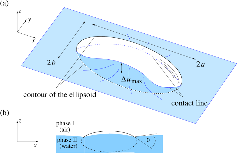
For in the range between 0 and 180o and in the absence of line tensions, the most stable configuration is given by the ellipsoid positioned flat on the interface (Fig. 1), because in this configuration the amount of displaced area of the air–water interface is maximal.111This can be shown by using the simplifying assumption that the interface around the ellipsoid remains flat Far03 . The meniscus deformation with respect to the plane is denoted by where is a two–dimensional vector in the plane and the vertical position of the ellipsoid center is given by . In order to determine the equilibrium deformation and vertical ellipsoid position, we seek an expansion of the free energy around a reference configuration characterized by the deformation and the vertical position such that
| (1) |
The properties of the reference configuration will be determined below. The change in free energy with respect to this reference configuration is given by
| (2) |
where denotes the change in meniscus area and denotes the change in contact area between the ellipsoid and air or water, respectively. We split this free energy difference into two parts:
| (3) | |||||
| (4) |
where the meniscus free energy denotes the difference of the air–water interfacial energy integrated over that part of the plane which is given by the area of the meniscus of the reference configuration projected onto it (denoted by ). The boundary free energy includes all remaining terms. We denote by the area of the meniscus projected onto the plane and describes the surface equation of the ellipsoid which depends on its vertical position as a parameter. With these definitions
At this point we perform a Taylor expansion up to second order in the meniscus deformation for the free energy contribution and separately. For , this is equivalent to the small–gradient expansion and results in
| (6) |
The expansion of the boundary part is somewhat more involved. Since the area of the domain will be of second order in the meniscus deformation, we can approximate in Eq. (2.1) and find
| (7) |
Here the functions and parametrize the polar radius of the boundaries and , respectively, i.e., they correspond to the projected three–phase contact lines formed by the reference meniscus and the arbitrary meniscus . Subsequently we perform a functional expansion of Eq. (7) with respect to displacements of the contact line position which are constrained to lie on the ellipsoid surface:
The position of the reference contact line is fixed by the requirement that the reference configuration minimizes , i.e.,
| (9) |
which leads to the following condition on :
| (10) |
Geometrically, Eq. (10) expresses the condition that at the reference contact line the angle between the unit vector in –direction and the ellipsoid normal is given by which is a reasonable first “guess” of the equilibrium contact line position. The solution to this equation yields ellipses for the projection of the reference contact line with half axes and . In order to fully specify the reference configuration, we require that the reference meniscus is a surface with minimal area, i.e, to first order it fulfills (consistent with Eq. (6)) with the pinning condition .
The second term on the r.h.s. of Eq. (2.1) gives us the approximation for the boundary free energy used in the following:
| (11) | |||||
| (12) |
Since it is a local functional on the projected reference contact line, this boundary free energy can be viewed as the total free energy cost in shifting the contact line with respect to the reference state. Thus we see that the minimization of the free energy , Taylor expanded to second order with given by Eq. (6) and by Eq. (11), with respect to leads to the linearized Young–Laplace equation (which also implies through ) with the local boundary condition on the projected reference contact line
| (13) |
Here, denotes the outward normal derivative on and is the line differential on . Through minimization of with respect to , the vertical position of the colloid is fixed by the condition
| (14) |
This condition implies that the solution does not depend on the choice of , the vertical position of the ellipsoid in the reference configuration. An arbitrary shift in will be compensated by a corresponding negative shift in , as can be shown from Eqs. (13) and (14).
At this point we want to remark that the reduction of the original capillary problem (with unknown contact line) to the solution of the Laplace equation with a local boundary condition at a fixed boundary (the projection of the reference contact line) is a great simplification and speeds up numerical solutions enormously. Furthermore we note that the technique of splitting the free energy into a meniscus and a boundary part with subsequent Taylor expansion has already been introduced in Ref. Oet05 for the problem of capillary deformations around colloidal spheres.
Since the boundary curve is itself an ellipse, a numerical solution for the meniscus deformation is most conveniently performed using elliptic coordinates whose relation to cartesian coordinates is given by and . Isolines of constant are ellipses, the condition that the boundary curve is such an isoline at leads to the relations and where is the eccentricity of the elliptic boundary curve. The Laplace equation in elliptic coordinates is given by
| (15) | |||||
| (16) |
and its solution is given by the expansion
where and denote elliptic multipole moments of order . Comparing to the general solution in polar coordinates,
we note that an elliptic multipole of order is a superposition of polar multipoles of order . In terms of the expansion given in Eq. (2.1), the problem reduces to a set of coupled linear equations for the multipole moments. It is usually sufficient to take into account multipoles of order for a very precise solution.
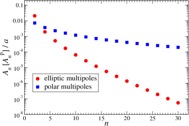
In Fig. 2 we compare the convergence of the elliptic and the polar multipole series for the meniscus deformation around an ellipsoid with aspect ratio and contact angle . The leading multipole is the quadrupole (). The vanishing monopole is related to the fact that no contact line force acts on the ellipsoid which we have ensured by minimizing the free energy with respect to the vertical position of the ellipsoid. The dipole moments are also zero since in equilibrium there is no torque acting on the ellipsoid. While the elliptic multipole expansion converges sufficiently fast for all practical purposes (e.g., ), the polar multipole series is very badly convergent (e.g., ). This is due to the fairly large aspect ratio; for the polar multipole series yields rapid convergence Nie05 .
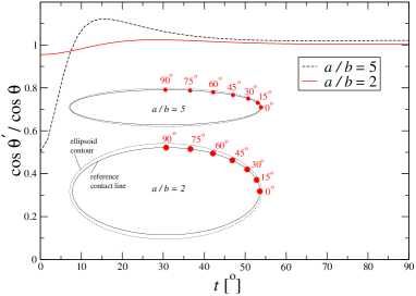
Due to the approximate forms of the meniscus and boundary free energy functionals (Eqs. (6) and (11)), Young’s condition is fulfilled only approximately for the corresponding minimum configuration. In general, the approximation becomes exact in the limit (for arbitrary aspect ratio ) or (for arbitrary contact angle ). The projected contact line of the approximate solution can be determined numerically by the intersection of the solution (2.1) with the ellipsoid. The likewise numerically determined contact angle varies along , for an example see Fig. 3 where the deviations from Young’s law are shown for an input contact angle and the two aspect ratios and . For the smaller value of the aspect ratio, the deviations are small. For however, larger deviations occur which are localized very close to the tips (in a domain , see the inset of Fig. 3). Closer inspection reveals that at the tips and on the contact line , the small–gradient approximation breaks down (however, it still holds approximately on the reference contact line ).
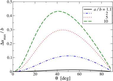
The meniscus shape strongly depends on the aspect ratio and the contact angle. We have investigated the influence of these parameters on the maximum height difference along the contact line, with the results shown in Fig. 4. This provides us with a quick estimate on the strength of the interaction between two ellipsoids since in linearized theory one can expect that the amplitude of the capillary interaction energy is approximately proportional to . Depending on the precise value of the aspect ratio, attains its maximum for contact angles between 40o and 55o, i.e. in the experiments of Ref. Lou06 , where for the used polystyrene ellipsoids a contact angle of around 40o was determined, the capillary deformation around the particles is close to its maximum as compared to particles of the same shape but with different .
2.2 Capillary interaction between two ellipsoids
For large distances , the capillary interaction between two ellipsoids is determined by the quadrupole. For small eccentricities () the interaction energy has been determined in Refs. Sta00 ; Fou02 and reads
| (19) |
where and are the polar orientation angles of the ellipsoids in the interface plane with respect to the distance vector between their centers (see Fig. 5 (a)). The simple energy estimate in Eq. (19) predicts that the corresponding forces between two ellipsoids approaching each other side–by–side () or tip–to–tip () are attractive and equal. However, an experimental estimate of these interaction forces Lou05 revealed that the attractive force in the side–by–side configuration varied as whereas for the tip–to–tip configuration it varied as , in accordance with Eq. (19). The measurements were performed over a limited distance range for aspect ratios ranging from 3 to 4.3.

Thus, for such aspect ratios the quadrupole approximation appears to be insufficient. We can apply the formalism developed in the previous subsection also to the evaluation of the interface deformation and associated capillary energy for two ellipsoids. The meniscus part of the free energy (Eq. (4)) remains unchanged save for the extend of the integration domain : here it consists of the whole plane with the two ellipses enclosed by the projected reference contact line cut out, .222We follow the convention of Ref. Oet05 and denote with a hat all quantities pertaining to the two–ellipsoid configuration. The boundary free energy for each ellipsoid (Eq. (11)) has to be amended by additional terms related to the appearance of an additional degree of freedom given by the angles of the long ellipsoid axis with the plane . For fixed distance and orientation angles and , the presence of the second ellipsoid causes the first ellipsoid to dip with its tip into the water and vice versa, i.e., the free energy has to be minimized with respect to rotations around an axis in the interface plane which is perpendicular to the symmetry axis. The additional terms in the boundary free energy can be determined as before in Sec. 2.1 by performing a Taylor expansion in terms of both, displacements of the contact line height and changes of the tilt angle around the reference configuration and (i.e., in the reference configuration the ellipsoids are positioned flat on the undisturbed interface). This procedure results in the expression
| (20) | |||||
for the total boundary free energy of two ellipsoids. The lengthy expressions for the coefficients , and are given in the appendix, see Eqs. (37)–(A). (Note that , Eq. (12).)
For two ellipsoids, the meniscus free energy of the reference configuration,
| (21) |
obviously depends on the configuration variables . The reference meniscus fulfills and the boundary condition . To include all dependence on the configuration variables into the total free energy, it is suitable to consider the free energy difference with respect to the reference state with :
| (22) | |||||
| (23) |
Consequently, the capillary potential can be defined as the free energy difference
| (24) |
The equilibrium configuration minimizes the free energy in Eq. (23) and can be calculated similarly as in Sec. 2.1. Minimizing with respect to and provides the equilibrium height and orientation of ellipsoid and leads to expressions analogous to Eq. (14) (since terms coupling and vanish). In contrast to the single colloid case, the equilibrium meniscus for two ellipsoids has to fulfill boundary conditions at both reference ellipses . They arise by minimizing the boundary free energy in Eq. (20) and contain an additional, -dependent term as compared to the boundary condition for the single ellipsoid (Eq. (13)). For the numerical determination of the equilibrium meniscus profile, the superposition ansatz is used. Thereby, the functions are given by the expansions of the meniscus around a single colloid into elliptic multipoles (Eq. (2.1)), and are elliptic coordinates with respect to the center of the reference ellipse (see Fig. 5). Through the boundary conditions a set of coupled linear equations for the multipole moments is derived which can be solved with standard numerical methods.
As an example for the results, the capillary force in direction of the distance vector between the ellipsoids is shown in Fig. 6, for an aspect ratio and a contact angle . The force considerably deviates from the quadrupole form for , i.e., in the region where the experimental measurements of Ref. Lou05 have been performed. For these distances, the force does not follow a power law but a fit to an effective power–law would clearly yield an exponent in the side–by–side configuration, but also an effective exponent for the tip–to–tip configuration. The reason for this behavior appears to be that the capillary deformation around one ellipsoid is dominated by the elliptic quadrupole, i.e., closer to the ellipsoid the capillary deformation has substantial contributions from polar multipoles higher than the quadrupole (see Fig. 2) which also influence the pair interaction considerably.
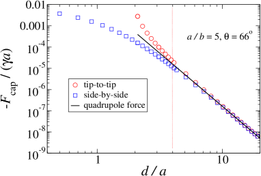
For the parameters used in Fig. 6 the asymptotic capillary potential, given by the quadrupole form , one finds the amplitude for ellipsoids with long half axis m at the air–water interface. Usually, the experimentally used ellipsoids are charge–stabilized which leads to an asymptotically isotropic dipolar repulsion . Using the results of Ref. Fry07 , one can estimate the amplitude of the electrostatic repulsions as (with a charge density of 1 electron per nm2 and ultrapure water). Thus the electrostatic repulsions are completely unimportant compared with the capillary potential; only for distances the directional capillary attractions would be overpowered by the electrostatic repulsions.
3 Capillary waves: fluctuation–induced interactions
As discussed in the introductory section, the scale of the fluctuation–induced interaction energies is such that they are observable only if static capillary interactions are (almost) absent. Since for the capillary interactions are identically zero (see the previous section) we discuss in this section the exemplary case of two ellipsoids with their centers at and their three–phase contact lines (ellipses with half axes and ) also located in the plane of the flat interface, corresponding to the equilibrium position of an ellipsoid with contact angle . Furthermore we assume that the contact line is pinned and the position of the ellipsoid is fixed by some external means. This corresponds to a Dirichlet boundary condition for the meniscus at the boundary of the projected meniscus area : . The free energy cost for small–gradient fluctuations of the interface position around its mean is given by the capillary wave Hamiltonian:
| (25) |
which (with ) has already been used for evaluating the free energy of static interface deformations (see Eq. (6)). In Eq. (25), denotes the capillary length which is usually much larger than the extensions of microcolloids, nevertheless it is necessary to keep the associated free energy contribution (stemming from gravity) throughout the calculations since it ensures the stability of the interface Leh07b . The capillary wave Hamiltonian depends on the position and orientation of the ellipsoids through the integration domain which encompasses the whole plane with the ellipses enclosed by the contact lines cut out. Therefore also the the free energy depends on the distance and the orientation angles and (see Fig. 5 (a)). The partition function is obtained by a functional integral over all possible interface configurations ; the boundary condition on the two contact lines and is included by -function constraints, as introduced in Ref. Li91 :
| (26) |
is a normalization factor such that . The -functions in Eq. (26) can be removed by using their integral representation via auxiliary fields defined on the contact lines Bor85 ; Li91 . This enables us to integrate out the field leading to
| (27) | |||||
Here, we introduced the Green’s function
of the operator
where is the modified Bessel function of the second kind.
In this form, the fluctuation part resembles 2d screened electrostatics: it is the
partition function of a system
of fluctuating charge densities residing on the contact lines.
In the intermediate asymptotic regime the free energy associated with this partition function can be calculated through an expansion of the auxiliary fields in terms of elliptic multipoles and an expansion of Green’s function in terms of using elliptic coordinates. Details of the lengthy calculations will be reported elsewhere. The resulting free energy can be written as an expansion with the two leading coefficients given by:
| (28) | |||||
| (29) |
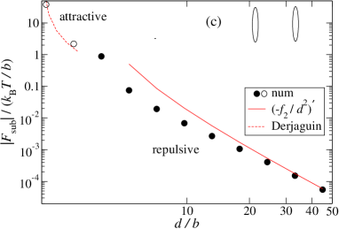
These expressions have been obtained in the limit which, however, is attained very slowly. In this limit the free energy difference is actually ill–defined and therefore the effective colloidal interaction is only meaningful for a finite capillary length , similar to a free two–dimensional interface the width of which is determined by the capillary wave fluctuations and diverges logarithmically . The leading terms of the fluctuation–induced free energy between spheres or disks (where the contact lines are circles of radius ) have already been calculated in Refs. Leh06 ; Leh07b and correspond to the orientation–independent terms in Eqs. (28) and (29) with . Note that for stretched ellipsoids with the next–to–leading order term in the free energy expansion may become repulsive when the ellipsoids are aligned side by side ().
In the opposite limit of small surface–to–surface distance the fluctuation force can be calculated by using the well–known result for the fluctuation force per length between two lines a distance apart Li91 , together with the Derjaguin (or proximity) approximation:
| (30) |
Here, and are the radii of curvature at those points on the contact line of ellipsoid 1 and 2, respectively, whose distance is the minimal surface–to–surface distance (see Fig. 5 (b)). Thus, the fluctuation–induced interaction energy between the ellipsoids diverges upon approach, similarly to the van–der–Waals attraction.
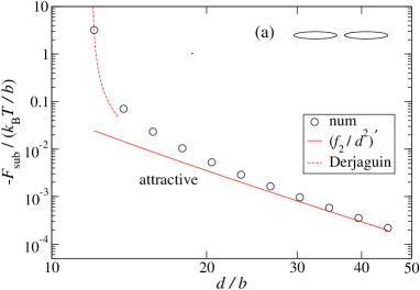
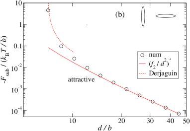
For intermediate distances the partition function must be evaluated numerically. In Eq. (26) the integral over the auxiliary fields can be carried out because they appear only quadratically in the exponent. The resulting determinant is divergent and requires regularisation. However, the derivative of its logarithm with respect to (corresponding to minus the force in direction of the distance vector between the centers of the ellipsoids) is finite and convergent in a numerical analysis (see Ref. Leh07b for further details). It turns out that the fluctuation force is attractive for all distances and orientations which were analyzed. This is already suggested by the close–distance regime (where is always attractive) and the long–distance regime (where is dominated by the likewise attractive, in–plane isotropic term , see Eq. (28)). In order to exemplify the effect of in–plane anisotropy on the fluctuation force, the results for the force with the asymptotically leading, isotropic term subtracted () are shown in Fig. 7 for ellipsoids with aspect ratio and for the three configurations (a) tip–to–tip (), (b) side–to–tip (, ) and (c) side–by–side (). For all configurations, for large the approach to the aymptotic result given by is fairly slow. For the configurations (a) and (b) the subtracted force remains attractive for all distances and there is a smooth crossover from the longe–distance to the close–distance regime while for the side–by–side configuration (c) there is a sign change from the attractive close–distance regime (open circles) to the repulsive long–distance regime (full circles), in accordance with Eq. (29).
4 Summary and conclusions
In this work we have analyzed the interface–mediated interactions which arise between ellipsoidal particles trapped at a fluid interface.
Firstly, ellipsoids cause static interface deformations if they are partially wetting and their contact angle is different from 90o. These static deformations lead to orientation–dependent capillary interactions between the particles. The full solution to this capillary problem requires the solution of a nonlinear differential equation together with Young’s condition on the boundary, the three–phase contact lines whose locations are a priori unknown. It is possible to analyze the interface deformation and the ensuing capillary potential in a perturbative treatment, valid for small deformations of the interface, which leads to the standard problem of a linear differential equation with a local condition on a given, fixed boundary. For small to intermediate distances between the ellipsoids we find considerable deviations from the well–known quadrupole interaction which is valid for asymptotically large distances. As a perspective for future work, the developed algorithm allows a fast determination of the deformation and the potential also for large eccentricities of the particles and appears to be potentially useful for application in computer simulations of the aggregation process in ellipsoidal monolayers.
Secondly, thermally excited capillary wave cause fluctuation–induced interactions between the ellipsoids. For the specific case of a pinned contact line we find that anisotropic effects in the fluctuation force arise only for subleading terms in an asymptotic expansion. It diverges for ellipsoids coming close to contact. However, due to its small scale the fluctuation force appears to be relevant experimentally only if the static capillary interactions are greatly reduced, e.g., if the ellipsoids are of nanometer size or the contact angle is close to 90o.
Acknowledgment: E. Noruzifar and M. Oettel thank the German Science
Foundation for financial
support
through the Collaborative Research Centre (SFB-TR6)
“Colloids in External Fields”.
Appendix A Contact line contributions to the free energy
In this appendix we determine the coefficients , and of the functional Taylor expansion of the boundary free energy in Eq. (20) around the reference configuration . They are given by the second variation of with respect to shifts of the contact line height or to changes in the orientation of the long axis of ellipsoid and can be calculated separately for the two colloids. As in Sec. 2.1 for the case of (for a single ellipsoid), the needed functional derivative , the derivative and the mixed derivative ) are determined by the derivatives of the boundaries of the surface integrals (given by the position of the three phase contact line, cf. Eq. (7)) with respect to and , respectively.
According to Eq. (7), , upon contact line shift and tilt the boundary free energy contains a contribution due to the change of the air–water interface (projected onto ):
| (31) |
and a contribution due to the change of the colloid area exposed to fluid I:
In Eq. (A), the surface integral is transformed into one over the cartesian components of a body–fixed coordinate system with axes fixed to the main ellipsoid axes for computational convenience in taking the derivatives. The reference contact line is parametrized by , (for ), and the shifted contact line is parametrized by .
The calculation of the boundary free energy variation can be performed in two steps: (1) First, we tilt ellipsoid by an angle with a pinned contact line. Then holds, but . (2) In a second step, the contact line is released to its final position . In this second step, both and , contribute to . The two steps have to be distinguished, since the orientational tilts change the surface measure of the ellipsoid. In order to avoid the calculation with the -dependent metric of the ellipsoid surface, we calculate the second variation in body–fixed coordinates of the colloid. The contribution from the change of the projected meniscus area is determined separately, here the steps (1) and (2) can be considered together. In body–fixed coordinates the metric is given by .
With being the height of the contact line relative to the center of colloid , the position of the three contact line in body–fixed coordinates after a shift of the contact line and a rotation of the ellipsoid by an angle (with respect to the plane ) is determined by the equations
| (33) | |||||
| (34) | |||||
| (35) |
parametrising the rotation, and the constraint
| (36) |
which ensures that the contact line is on the ellipsoid surface.
Employing the relations given above we can calculate the contact line position on the rotated ellipsoid and, in particular, its partial derivatives. After some algebra, we finally arrive at the expressions
| (37) | |||||
| (38) | |||||
and
for the coefficients of the functional Taylor expansion of . Here, .
Note, that by minimizing with respect to we ensure torque balance of the colloid whereas mimimizing with respect to the height guarantees that the total vertical force exerted by the meniscus on the contact line vanishes. The numerical calculation of the equilibrium meniscus between two ellipsoidal particles and the resulting capillary interactions shows, however, that the effect of is rather small, leading to changes of the results as compared to the computations using the boundary contribution (13), in which is neglected.
References
- (1) P. A. Kralchevsky and K. Nagayama, Adv. Coll. Interface Sci. 85, 145 (2000).
- (2) F. Bresme and M. Oettel, J. Phys.: Condens. Matter 19, 413101 (2007).
- (3) M. Oettel and S. Dietrich, Langmuir ASAP, eprint http://pubs.acs.org/cgi-bin/abstract.cgi/langd5/asap/abs/la702794d.html (2008).
- (4) L. Foret and A. Würger, Phys. Rev. Lett. 92, 058302 (2004).
- (5) A. Dominguez, M. Oettel, and S. Dietrich, J. Phys.: Condens. Matter 17, S3387 (2005).
- (6) A. Dominguez, M. Oettel, and S. Dietrich, Europhys. Lett. 77, 68002 (2007).
- (7) M. Oettel, A. Dominguez, and S. Dietrich, J. Phys.: Condens. Matter 17, L337 (2005).
- (8) A. Würger and L. Foret, J. Phys. Chem. B 109, 16435 (2005).
- (9) D. Frydel, S. Dietrich, and M. Oettel, Phys. Rev. Lett. 99, 118302 (2007).
- (10) J.-P. Fournier and P. Galatola, Phys. Rev. E 65, 031601 (2002).
- (11) P. Yang and F. Kim, ChemPhysChem 3, 503 (2002).
- (12) A. B. Brown, C. G. Smith, and A. R. Rennie, Phys. Rev. E 63, 016305 (2001).
- (13) J. C. Loudet, A. M. Alsayed, J. Zhang, and A. G. Yodh, Phys. Rev. Lett. 94, 018301 (2005).
- (14) M. G. Basavaraj, G. G. Fuller, J. Fransaer, and J. Vermant, Langmuir 22, 6605 (2006).
- (15) J. C. Loudet, A. G. Yodh, and B. Pouligny, Phys. Rev. Lett. 97, 018304 (2006).
- (16) E. A. van Nierop, M. A. Stijnman, and S. Hilgenfeldt, Europhys. Lett. 72, 671 (2005).
- (17) D. Stamou, C. Duschl, and D. Johannsmann, Phys. Rev. E 62, 5263 (2000).
- (18) K. D. Danov, P. A. Kralchevsky, B. N. Naydenov, and G. Brenn, J. Colloid Interf. Science 287, 121 (2005).
- (19) H. Lehle, M. Oettel, and S. Dietrich, Europhys. Lett. 75, 174 (2006).
- (20) H. Lehle and M. Oettel, Phys. Rev. E 75, 011602 (2007).
- (21) R. Golestanian, M. Goulian, and M. Kardar, Phys. Rev. E 54, 6725 (1996).
- (22) M. Goulian, R. Bruinsma, and P. Pincus, Europhys. Lett. 22, 145 (1993); 23, 155(E) (1993).
- (23) J. Faraudo and F. Bresme, J. Chem. Phys. 118, 6518 (2003).
- (24) M. Oettel, A. Dominguez, and S. Dietrich, Phys. Rev. E 71, 051401 (2005).
- (25) M. Bordag, D. Robaschik, and E. Wieczorek, Ann. Phys. 165, 192 (1985).
- (26) H. Li and M. Kardar, Phys. Rev. Lett. 67, 3275 (1991).