Collapse and revivals of the photon field in a Landau-Zener process

Abstract

We consider the evolution of a two-level system coupled to a photon field initially in a coherent state, as the energy of the two-level system is linearly varied through resonance with the photon field. At a fixed time after the resonance, the amplitude of the photon field is found to show a collapse and subsequent revivals as a function of rate of energy variation. Including decay of the photon field, we find that the observation of such collapse and revivals is near the technological limit of current cavity QED experiments but should be achievable.

The famous problem of Landau Landau (1932) and Zener Zener (1932) concerns a two-level system whose parameters are varied so that an anticrossing of energy levels occurs, and provides the probability that the system will remain in an adiabatic state. There has been much work since on finding generalisations of this problem to many levels which can still be exactly solved, e.g Brundobler and Elser (1993); Shytov (2004); Volkov and Ostrovsky (2004, 2005); Dobrescu and Sinitsyn (2006). Another generalisation of the Landau Zener process is to consider multiple occupation of single particle levels, and then to find how varying the single particle level energies affects the many particle stateAltland and Gurarie (2008). These constitute a large class of possible problems, of which we study a particular case relevant to cavity QED experiments Mabuchi and Doherty (2002); Blais et al. (2004); Brennecke et al. (2007); Auffeves et al. (2003); Raimond et al. (2001). Cavity QED studies strong light-matter coupling between photons confined in a cavity and matter (e.g. single atoms, or artificial atoms such as quantum dots Khitrova et al. (2007) or Josephson junctions Blais et al. (2004)). We consider a cavity QED system in which the matter is driven through a Landau-Zener transition, and find that this has dramatic consequences for the state of the photon field: observing at a fixed time after the anticrossing and changing the rate of energy variation, there is a collapse and revival of the photon field amplitude. These oscillations extend far into the regime of slow energy variation — the adiabatic limit — in which the single particle Landau-Zener probability shows no further change.

The scheme we propose consists of a two-level system coupled to a photon mode in a cavity; the energy of the two-level system is varied linearly in time, passing through resonance with the photon energy. A related problem, but with a classical photon field, was considered in Ref. Wubs et al. (2005); we also note that a generalisation of our model to many two-level systems is analogous to models of interest describing production of molecules in cold atomic gases, when varying the molecular energy by a Feshbach resonance, e.g.Barankov and Levitov ; Altman and Vishwanath (2005); Altland and Gurarie (2008); Sun et al. . If the initial cavity state were a number state then the result would be the Landau-Zener energy level crossing: The state with an excited two-level system and $n-1$ photons crosses the state with an unexcited two-level system and $n$ photons; the mutual repulsion of these states is given by $g\sqrt{n}$, where $g$ is the radiation-matter coupling strength. Varying the two-level system energy linearly in time as $E=\lambda t$ induces transitions between these states. The standard Landau-Zener result Landau (1932); Zener (1932) is that in terms of the parameter $z=g^{2}/\lambda$, the probability of remaining in the lowest energy state (rather than exciting the system) is $P=1-e^{-2\pi zn}$. If the energy ramp is slow, or $zn\gg 1$, this quickly saturates at $1$.

However, a natural state of the cavity is the coherent state Scully and Zubairy (1997), leading to a far more intricate behaviour. The coherent state can be resolved onto a basis of number states, and each number state evolves independently. The effective radiation-matter coupling strength for $n$ photons is $g\sqrt{n}$, and so the evolution of each photon number state is also $n$ dependent. In particular, each photon number state acquires a different phase during the process; this phase difference continues to play an important role even when the sweep velocity is so slow that $z\gg 1$ and the probability for a single transition $P=1-e^{-2\pi zn}\simeq 1$. To measure the effect of these phase differences, the easiest quantity to measure is the amplitude of the resultant photon field, $\langle\hat{\psi}\rangle=\langle\Psi|\hat{\psi}|\Psi\rangle$. How this is to be measured depends on the particular cavity QED system used. Some possible methods include Ramsey interferometry of a second atom to probe the state of the cavity Raimond et al. (2001); homodyne measurement of the photons leaking out of the cavity by interfering it with a reference beam; and homodyne measurement inside the cavity by detecting the interfering fields with a second atom Auffeves et al. (2003). The dependence of this field amplitude on the rate of sweeping is shown in Fig. 1, for two different values of the initial field amplitude.

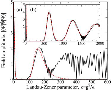
Figure 1: Dependence of the photon field intensity on the Landau-Zener parameter, $z=g^{2}/\lambda$. Main figure, initial coherent state amplitude $\psi=5$; inset $\psi=10$. The red dashed line is the approximation discussed in the text.

The photon field amplitude shows a collapse and subsequent revivals arising from the phase difference between different number state components of the coherent state. The collapse occurs as, with slower driving, the phase difference between different number states grows, and so their contributions to the field amplitude interfere destructively. At yet slower driving, the phase difference grows sufficiently that subsequent number states are back in phase. However, since the dependence of the phase on photon number is nonlinear, these revivals are imperfect, and eventually cease.

Let us now discuss this behaviour more quantitatively; the Hamiltonian of the problem is:

$$\hat{H}=\omega_{0}\,\hat{\psi}^{\dagger}\hat{\psi}+\frac{\lambda t}{2}\hat{\sigma}_{z}+g\left(\hat{\psi}^{\dagger}\hat{\sigma}^{-}+\hat{\psi}\,\hat{\sigma}^{+}\right),$$ (1)

At the beginning of the time evolution, the two-level system energy is well below the photon energy and the system is initialised in a coherent photon state, $\left|\Psi_{i}\right>=e^{-|\psi|^{2}/2}\sum_{n}(\psi^{n}/\sqrt{n!})\left|n,\uparrow\right>.$ Evolution under Eq. (1) gives $\left|n,\uparrow\right>\to A_{n+1}\left|n,\uparrow\right>+B_{n+1}\left|n+1,\downarrow\right>$, where for evolution from $-T$ to $T$ for large times $T$, the coefficientsZener (1932); Vitanov and Garraway (1996) are:

$$A_{n} =e^{-n\pi z},$$ (2)

$$B_{n} =\frac{\sqrt{2\pi nz}e^{-n\pi z/2}}{\Gamma(1-inz)}e^{-i\left[\pi/4+\lambda T^{2}/2+2zn\ln(\sqrt{\lambda}T)\right]}.$$ (3)

In the large $z$ limit where interesting behaviour is seen in Fig. 1, $A_{n}\simeq 0$ and $|B_{n}|\simeq 1$ so we may write $B_{n}=\exp(i\phi_{n})$ with $\phi_{n}(T)=zn\left[\ln(zn)-1\right]-2zn\ln(\sqrt{\lambda}T)+\phi_{0}$. In this adiabatic limit, this phase is just the integral of $E_{n}(t)$, the instantaneous energy of the eigenstate with $n$ excitations. The final many body state is then: $\left|\Psi\right>=e^{-|\psi|^{2}/2}\sum_{n}(\psi^{n}e^{i\phi_{n+1}(T)}/\sqrt{n!})\left|n+1,\downarrow\right>.$ The measurable field amplitude can then be written as

$$\left<\hat{\psi}\right>=\psi e^{-|\psi|^{2}}\sum_{n}\frac{|\psi|^{2n}}{n!}\sqrt{\frac{n+2}{n+1}}e^{i(\phi_{n+2}-\phi_{n+1})}$$ (4)

The existence and explanation of the collapse and revivals here is related to the collapse and revival of Rabi oscillations Narozhny et al. (1981); Gea-Banacloche (1990); Phoenix and Knight (1991); this occurs in a model like Eq. (1) but without time-varying energies, and collapse and revivals occur as a function of time. Let us discuss the case $\left|\psi\right|^{2}\gg 1$. As in Narozhny et al. (1981), one can expand the phase difference $\Delta\phi_{n}=\phi_{n+1}-\phi_{n}$ near $n=|\psi|^{2}$ (where the amplitude of the terms in the sum peaks), giving $\Delta\phi_{|\psi|^{2}+m}=\Delta\phi_{|\psi|^{2}}+zm/|\psi|^{2}-zm^{2}/(2|\psi|^{4}).$ The revivals in Fig. 1 occur when $\Delta\phi_{n}$ is the same (modulo $2\pi$) for each term in Eq. (4); for small $m$ this condition is $z=2\pi N|\psi|^{2}$, where $N$ is an integer labelling the revival. Near such revivals, after subtracting $2\pi Nm$ from $\Delta\phi_{|\psi|^{2}+m}$, it can be written so it varies slowly with $m$:

$$\Delta\phi_{|\psi|^{2}+m}-2\pi Nm=\Delta\phi_{|\psi|^{2}}+\frac{(z-2\pi N|\psi|^{2})m}{|\psi|^{2}}-\frac{zm^{2}}{2|\psi|^{4}}.$$

This then allows the sum in Eq. (4) to be replaced with an integral over $m=n-|\psi|^{2}$. Using the Gaussian approximation to the Poisson distribution, yields:

$$\left<\hat{\psi}\right>=\int_{-\infty}^{\infty}\frac{dm}{\sqrt{2\pi}}\exp\left[-\frac{m^{2}}{2|\psi|^{2}}+i\Delta\phi_{|\psi|^{2}+m}\right].$$

Evaluating this Gaussian integral, and summing over values of $N$ for each revival gives the result:

$$\left|\left<\hat{\psi}\right>\right|=\frac{|\psi|}{\sqrt[4]{1+z^{2}/|\psi|^{4}}}\!\sum_{N=0}^{N_{\text{max}}}\!\!\exp\left[\frac{-(z-2\pi N|\psi|^{2})^{2}}{2|\psi|^{2}(1+z^{2}/|\psi|^{4})}\right].$$ (5)

At very large $z$, the revivals disappear and the behaviour becomes complex because terms of higher order in $m$ in the expansion of $\Delta\phi_{|\psi|^{2}+m}$ play a role when $z\gtrsim 3|\psi|^{3}$. This means revivals are not seen for $N>N_{\text{max}}\approx|\psi|/2$. Equation (5) is shown in Fig. 1 by the red dashed line.

The revivals seen in the field amplitude do not indicate a complete revival of the initial coherent state. This can be seen by considering the Wigner function Scully and Zubairy (1997), $W(x,p)=\int\Psi^{\ast}(x+y)\Psi(x-y)e^{2ipy}dy/\pi$, where $\Psi(x)=\langle x|\Psi\rangle$ is the position representation of the photon wavefunction, and can be written in terms of Hermite polynomials $H_{n}(x)$ (which correspond to number states) as:

$$\Psi(x)=\frac{e^{-(|\psi|^{2}+x^{2})/2}}{\pi^{1/4}\psi}\sum_{n=1}^{\infty}\frac{\psi^{n}e^{i\phi_{n}(T)}}{\sqrt{2^{n}}(n-1)!\sqrt{n}}H_{n}(x).$$ (6)

As seen in Fig. 2, as soon as $z\gg 1$ the Wigner function has many nodes, and describes a highly non-classical state, unlike the initial coherent state whose Wigner function is a Gaussian Scully and Zubairy (1997). We note that unlike the collapse and revival of Rabi oscillations Gea-Banacloche (1990); Phoenix and Knight (1991) this non-classical state is not associated with entanglement between the two-level system and photon field Brune et al. (1996) at the end of the dynamics, although transient entanglement does occur during the sweep. Since the collapse and revival occur in the adiabatic limit the two-level system always ends in a pure state and so (in the absence of decay) the photon state is a pure but non-classical state. The complete Wigner function can be measured by quantum state tomography Vogel and Risken (1989); Smithey et al. (1993); such measurements have recently been performed in cavity QED experiments Bertet et al. (2002); Houck et al. (2007).

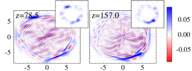
Figure 2: Wigner function of the final photon state for $\psi=5$ at values of $z$ corresponding to the first collapse and first revival. Inset: Glauber Q function on same scale for same parameters.

In a real cavity QED experiment there is decoherence due to escape of photons out of the cavity, and decay of the two-level system without emitting a photon; these may present an obstacle to observing the revivals, and so we next investigate the maximum photon loss rate $\kappa$ and non-radiative decay rate $\gamma$ that can be tolerated. With a non-zero decay rate $\kappa$, one must consider an finite duration of the level crossing, and to maximise the signal one should make the duration as short as possible consistent with accumulating the necessary phase. A naive estimate of the effect of decay comes from $(\kappa t^{\ast},\gamma t^{\ast})$ where $t^{\ast}$ is the time for the level crossing to occur, given by $\lambda t^{\ast}\simeq g|\psi|$, and $g|\psi|$ is the characteristic coupling strength for the coherent photon state. Decay is weak if $(\kappa t^{\ast},\gamma t^{\ast})\ll 1$, which gives $(\kappa,\gamma)/g\ll(\lambda/g^{2})/|\psi|$. For this condition to be satisfied at the first revival, when $g^{2}/\lambda=z=2\pi|\psi|^{2}$, one requires that $(\kappa,\gamma)/g\ll 1/(2\pi|\psi|^{3})$. Away from the level crossing the effects of decay are less serious; decay after the crossing attenuates the amplitude of the signal, decay beforehand reduces the amplitude of the initial photon field amplitude. This naive estimate is sufficient for the effects of non-radiative decay, but not for loss of photons.

To investigate the effects of decay quantitatively, we solve numerically the density matrix equation of motion:

$$\partial_{t}\hat{\rho}=-i\left[\hat{H},\hat{\rho}\right]+\mathcal{L}_{\kappa}[\hat{\rho}]+\mathcal{L}_{\gamma}[\hat{\rho}]$$ (7)

where $\mathcal{L}_{\kappa}[\hat{\rho}]=(\kappa/2)[\hat{\psi}^{\dagger}\hat{\psi}\hat{\rho}+\hat{\rho}\hat{\psi}^{\dagger}\hat{\psi}-2\hat{\psi}\hat{\rho}\hat{\psi}^{\dagger}]$ describes loss of photons and $\mathcal{L}_{\gamma}[\hat{\rho}]=(\gamma/2)[\hat{\sigma}_{+}\hat{\sigma}_{0}\hat{\rho}+\hat{\rho}\hat{\sigma}_{+}\hat{\sigma}_{-}-2\hat{\sigma}_{-}\hat{\rho}\hat{\sigma}_{+}]$ describes non-radiative decay of spins Scully and Zubairy (1997). The numerical solution of this equation, shown in Fig. 3, reveals a greater effect of photon loss than the naive estimate above. For $\psi=5$, the maximum permissible decay rates is $\kappa/g\simeq 2\times 10^{-5}$, $\gamma/g\simeq 2\times 10^{-4}$, compared to the naive estimate $1/(2\pi|\psi|^{3})\simeq 10^{-3}$.

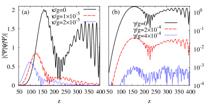
Figure 3: Effect of decay on $z$ dependence of field amplitude. Left panel: effect of photon leakage, $\kappa$. Right panel: effect of non-radiative decay $\gamma$ (with field amplitude plotted on logarithmic scale). Plotted for $\psi=5$ and a time range of $-10^{4}<gt<10^{4}$.

To understand this enhancement of decay, it is convenient to calculate the effect of photon decay in the adiabatic limit, such that the state $\left|n-1,\uparrow\right>$ evolves to:

$$\left|n,+\right> =\left[\cos(\theta_{n})\left|n,\downarrow\right>+\sin(\theta_{n})\left|n-1,\uparrow\right>\right]$$ (8)

$$\cos(\theta_{n}) =\sqrt{\frac{1}{2}\left[1+\frac{\tau}{\sqrt{n+\tau^{2}}}\right]},\quad\tau=\frac{\lambda t}{2g}.$$ (9)

The adiabatic approximation is appropriate even with photon decay because the probability that loss of a photon swaps between the $|+\rangle$ and $|-\rangle$ subspaces is small. This probability, of switching from $|n,+\rangle$ to $|n-1,-\rangle$ is given by: $P_{-+}=|\langle n-1,-|\hat{\psi}|n,+\rangle|^{2}/\langle n,+|\hat{\psi}^{\dagger}\hat{\psi}|n,+\rangle$ and can be written in terms of the $\theta_{n},\tau$ of Eq. (9) as:

$$P_{-+} =\frac{|\cos(\theta_{n})\sin(\theta_{n-1})\sqrt{n}-\sin(\theta_{n})\cos(\theta_{n-1})\sqrt{n-1}|^{2}}{n-\sin^{2}(\theta_{n})}$$

$$\approx\frac{1}{16n^{2}}\left[\frac{\tau\sqrt{n}}{n+\tau^{2}}-\sqrt{\frac{n}{n+\tau^{2}}}\right]^{2}\leq\frac{1}{16n^{2}}\frac{27}{16}.$$ (10)

where the last expression makes use of approximations for $n\gg 1$. It is thus clear that for large $n$, the probability of leaving the adiabatic subspace is small.

In this adiabatic subspace, the density matrix equation gives a closed set of equations for off-diagonal terms, $\Lambda_{n}=\left<n-1,+|\hat{\rho}|n,+\right>$, and the measured field amplitude is $\langle\Psi|\hat{\psi}|\Psi\rangle=\sum_{n}\sqrt{n}\Lambda_{n}$. The effect of the Hamiltonian is phase evolution of each $\Lambda_{n}$, with the final phase gain of $\Lambda_{n}$ being $\Delta\phi_{n-1}(T)$ as in Eq. (4). Including also the matrix elements due to photon decay, one can write:

$$\frac{d\Lambda_{n}}{dt}=i\frac{d\Delta\phi_{n-1}}{dt}\Lambda_{n}-\kappa\left[\left(n-\frac{1}{2}\right)\Lambda_{n}-\sqrt{n^{2}+n}\Lambda_{n+1}\right]$$ (11)

For the range of parameters shown in Fig. 3(a), the results of numerical evaluation of this equation and of the full problem, Eq. (7) cannot be distinguished by eye.

If $\kappa=0$, the solution for $\Lambda_{n}$ recovers Eq. (4). Alternatively, if $\Delta\phi_{n}$ is time independent, then for an initial coherent state, the time evolution can also be exactly solved Scully and Zubairy (1997) and the field amplitude decays as $\psi(t)=\psi(0)e^{-\kappa t/2}$. It may appear surprising that the characteristic decay rate is $\kappa$, while the apparent rate in Eq. (11) is $\kappa n$; the explanation is that the order $n$ contributions from the $\Lambda_{n}$ and $\Lambda_{n+1}$ terms cancel. However, with a time-dependent $\Delta\phi_{n}$, the $\Lambda_{n}$ and $\Lambda_{n+1}$ terms pick up a relative phase difference, and the cancellation of the order $n$ term fails. Thus the characteristic decay rate is $\kappa n\simeq\kappa|\psi|^{2}$ during the level-crossing time, hence the actual requirement for small decay is $\kappa/g\ll 1/(2\pi|\psi|^{5})$; for $\psi=5$ this gives $\kappa/g\ll 5\times 10^{-5}$ (cf Fig. 3).

Of the various realisations of cavity QED, those with parameters closest to those required by the constraints on $\kappa/g,\gamma/g$ are either Josephson junctions coupled to stripline resonatorsBlais et al. (2004), or Rydberg atoms in microwave cavities Kuhr et al. (2007). For Rydberg atoms the values of $\kappa/g$, $\gamma/g$ currently achievable are very close to those required, but the limiting factor is the short time taken for an atom to pass through the cavity.

Finally, let us present a more quantitative understanding of the “enhanced decay” by comparing the perturbative solution of Eq. (11) to the naive expectation:

$$\left<\Psi|\hat{\psi}(\kappa,\psi_{0})|\Psi\right>_{\text{naive}}=\left<\Psi|\hat{\psi}(0,\psi_{0}e^{-\kappa T/2})|\Psi\right>e^{-\kappa T/2}$$ (12)

This naive decay describes decay of the initial coherent state before the anticrossing (thus shifting the revivals to smaller values of $z$), and decay of the field amplitude after the anticrossing. The perturbative solution (to leading order in $\kappa$) of Eq. (11) can be easily found by writing $\Lambda_{n}=\tilde{\Lambda}_{n}\exp[-i\Delta\phi_{n-1}(t)]$, and then ignoring the $\kappa$ dependence of $\tilde{\Lambda}_{n}$ on the right hand side of Eq. (11). It will be convenient to write the initial conditions for $\Lambda_{n}$ as $\Lambda_{n}=P_{n}\psi/\sqrt{n}$, where $P_{n}=e^{-|\psi|^{2}}|\psi|^{2(n-1)}/(n-1)!$ is the probability of having $n-1$ photons. Writing $\delta\langle\Psi|\hat{\psi}|\Psi\rangle=\langle\Psi|\hat{\psi}|\Psi\rangle_{\text{naive}}-\langle\Psi|\hat{\psi}|\Psi\rangle$ and expanding both Eq. (12) and the solution to Eq. (11) to leading order in $\kappa$, one has:

$$\delta\langle\Psi|\hat{\psi}|\Psi\rangle=\kappa|\psi|^{2}\sum_{n}P_{n}\psi\times\\ \left[\vphantom{\int}Te^{i[\Delta\phi_{n-1}(-T)-\Delta\phi_{n-1}(T)]}+Te^{i[\Delta\phi_{n}(-T)-\Delta\phi_{n}(T)]}\right.\\ \left.-e^{i[\Delta\phi_{n}(-T)-\Delta\phi_{n-1}(T)]}\int_{-T}^{T}e^{i[\Delta\phi_{n-1}-\Delta\phi_{n}]}dt\right]$$ (13)

Assuming $n\gg 1$, one can simplify the expressions for the phase differences appearing here to give:

$$\delta\langle\Psi|\hat{\psi}|\Psi\rangle=\kappa|\psi|^{2}\sum_{n}P_{n}\psi e^{-iz\ln(T^{2}/zn)+iz/2n}\times\\ \int_{-T}^{T}dt\left[\cos\left(\frac{z}{2n}\right)-\cos\left(\frac{z}{2n}\frac{\sqrt{\lambda}t/2}{\sqrt{zn+\lambda t^{2}/4}}\right)\right]$$ (14)

Finally, note that the integral in Eq. (14) has a finite limit as $T\to\infty$; this means that the naive decay that was subtracted fully describes the decay at long times, and Eq. (14) describes only the extra contribution that occurs during the crossing. Taking $T\to\infty$, the integral can be found in terms of a Bessel function yielding:

$$\delta\!\langle\Psi|\hat{\psi}|\Psi\rangle=-\kappa|\psi|^{2}\pi\times\\ \sum_{n}P_{n}\psi e^{-iz\ln\left(\frac{T^{2}}{zn}\right)+i\left(\frac{z}{2n}\right)}\sqrt{\frac{z^{3}}{n\lambda}}J_{1}\left(\frac{z}{2n}\right)$$ (15)

Using the asymptotic form for the Bessel function, this expression shows that the characteristic scale of the extra decay is given by: $\delta\!\langle\Psi|\hat{\psi}|\Psi\rangle\propto\kappa|\psi|^{2}\psi z/\sqrt{\lambda}\propto(\kappa/g)|\psi|^{3}z^{3/2}$. This extra term explains both the scale of the extra decay observed in Fig. 3(a), and also the $z$ dependence of the decay visible in that figure.

In summary we have proposed an experiment in which collapse and revivals of a coherent field amplitude can be seen as a function of varying sweep rate in a Landau-Zener level crossing problem. Considering a leaky cavity and non-radiative decay, this effect continues to survive as long as decay is weak enough, however the sense of “weak enough”, $\kappa/g\leq 10^{-5}$, differs from the naive expectation. As such, this proposed experiment is at the limit of the capability of current experiments, and so provides a dramatic consequence to be observed by any system far in the strong-coupling limit