Parameter-tuning Networks: Experiments and Active Walk Model

Abstract

The tuning process of a large apparatus of many components could be represented and quantified by constructing parameter-tuning networks. The experimental tuning of the ion source of the neutral beam injector of HT-7 Tokamak is presented as an example. Stretched-exponential cumulative degree distributions are found in the parameter-tuning networks. An active walk model with eight walkers is constructed. Each active walker is a particle moving with friction in an energy landscape; the landscape is modified by the collective action of all the walkers. Numerical simulations show that the parameter-tuning networks generated by the model also give stretched exponential functions, in good agreement with experiments. Our methods provide a new way and a new insight to understand the action of humans in the parameter-tuning of experimental processes, is helpful for experimental research and other optimization problems.

Large apparatuses pay more and more important role in the experimental research of modern physics, such as the high-energy accelerators and controlling nuclear fusion devices. A large apparatus made up of many components, each component needs be tested and tuned separately and then collectively, before experiments using the apparatus as a whole can be conducted. And there are a large number of parameters to be tuned. The parameter tuning processes are often complicated and onerous, strongly depend on the the experience of experimenter. How can we model the adjustment process of these parameters and make some sense out of it?

For example, in a Tokamak in plasma physics, in the ion source segment of the neutral-beam injector system alone, there are eight major parameters to be adjusted. The experimenter sets the parameter values, turns on the equipment, and measures the outcome of a certain quantity $Q$. If the $Q$ obtained does not meet the mark $Q_{0}$, say, the whole process is repeated, with a new set of parameters. The adjustment process stops when $Q$ is equal or very close to $Q_{0}$. The simultaneous adjustment of a large number of parameters is a complicated process, which is based on the feedback from previous $Q$ values obtained, the experimenter’s experience, and the limitation of the hardware that control the parameters.

To quantify this complicated process, a parameter-tuning network can be constructed as follows. Assume that $N$ parameters $u_{i}(i=1,2,\cdots,N)$ are involved. The experimenter’s serial adjustment of u $[\equiv(u_{1},\cdots,u_{N})]$ can be represented by a sequence of connected dots in the $N$-dimensional u space. For each choice of u, $Q$ is measured, so that $Q=Q(\emph{{u}})$ but the functional form is unknown due to the complexity of the equipment, which is like a black box.

The sequence of u dots is then projected onto the $(u_{1},u_{2})$ plane, say. The dots on the same vertical line along the $u_{3}$ direction are allowed to collapse to one point, called a node. A line connecting two nodes is called an edge Wat1 ; Bar1 ; Bar2 . Since in real situations, the parameters selected by the experimenter in different adjustments may partially overlap with each other, there may be more than one edge connecting two nodes. These edges are directed. For simplicity, we make the approximation of collapsing all the edges between two nodes that have the same direction as one single edge with the same direction. Consequently, between two nodes, there are at most two edges with opposite directions, resulting in a directed parameter-tuning network. A non-directed network is formed from the directed one, by collapsing all the edges between any two nodes and removing the directions.

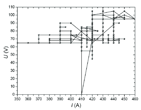
Figure 1: The non-directed parameter network on the (U, I) plane derived from the experimental data, where U is the working voltage of the cathode gas valve and I the filament current.

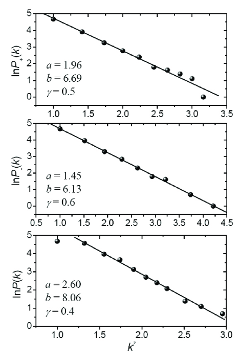
Figure 2: Experimental curves of $P_{+}(k)$, $P_{-}(k)$ and $P(k)$, fitted to stretched exponent functions. The corresponding (directed and non-directed) parameter-tuning networks exist on the (U, I) plane, where U is the working voltage of the cathode gas valve and I the filament current. Its non-directed structure has been shown in FIG. 1. The experimental data obtained from the tuning of the ion source in a whole experiment season, the sequence includes 789 parameter sets.

In a parameter-tuning network, there are $N_{n}$ nodes, say. For a directed parameter-tuning network node $j(j=1,2,\cdots,N_{n})$, let $N_{+}(j)$ be the number of in-going edges, $N_{-}(j)$ the number of out-going edge.

Now count the number of $N_{+}$ that has the value $k$, and call it $p_{+}(k)$; similarly for $p_{-}(k)$. The corresponding function in the non-directed network case is denoted by $p(k)$. $k$ is called the ”degree” of a node. $p_{+}(k)$ is called the ”in-degree distribution”, $p_{-}(k)$ the ”out-degree distribution”, and $p(k)$ the ”degree distribution.” Next define the corresponding ”culmulative degree distributions” $P_{+}(k)$, $P_{-}(k)$ and $P(k)$ by

$$P_{+}(k)\equiv\sum_{k^{\prime}=k}^{k_{m}}p_{+}(k^{\prime})\\$$ (1)

$$P_{-}(k)\equiv\sum_{k^{\prime}=k}^{k_{m}}p_{-}(k^{\prime})\\$$ (2)

$$P(k)\equiv\sum_{k^{\prime}=k}^{k_{m}}p(k^{\prime})\\$$ (3)

Here $k_{m}$ is the maximum $k$ that the $p$ function is non-zero, and all of the distribution functions are not unitary. Note that by definition, the $P$’s are monotonic decreasing functions, while the $p$’s may not be monotonic at all. The reason for introducing the $P$’s is that we want to fit them to monotonic decreasing functions such as stretched exponents or power laws.

In our experiments studying the ion source of neutral beam injector system for HT-7 Tokamak, eight control parameters are involved $(N=8)$. These include the filament current, magnet current, arc voltage, cathode gas valve voltage, anode gas valve voltage, etc. Each of the parameters has 10 to 30 discrete, adjustable setting values. The aim of the experiment is to find out which set of parameters will give a strong and stable discharge, measured by the arc current intensity $Q$. Each parameter is set by a dial which can be turned left or right between two extreme positions. When the extreme position is reached, the experimenter has to turn the dial back, reversing the direction of turning.

From our experimental data, the sequence of parameters in the 8-dimensional u space is first generated and the corresponding directed and non-directed tuning-parameter networks are constructed. The non-directed network is shown in FIG. 1. The $P$’s are obtained, and fitted nicely with stretched exponential functions (FIG. 2) such that

$$P(k)\sim\exp(-ak^{\gamma})$$ (4)

or, equivalently,

$$\ln P(k)=-ak^{\gamma}+b$$ (5)

and similarly for $P_{+}(k)$ and $P_{-}(k)$. Such property is also found in the parameter-tuning networks derived from the data of the tuning experiments in other experiment season of the ion source (each of them includes 600 to 800 parameter sets).

The experimental adjustment of the parameters is somehow correlated by the experimenter, and the process can be modeled by an active walk (AW) model Lam2 . In our AW model here, $N=8$; each $u_{i}$ has adjustable values of $1,2,\cdots,20$, say. The adjustment of the $i$th parameter is represented by the movement of an active walker on a 1D landscape potential $V_{i}(x_{i})$. The allowable $x_{i}$ for the $i$th walker are the integers $(1,2,3,\cdots,100)$, the same for all $i$. These 100 numbers are mapped to the $u_{i}$, such that if the $i$th walker ends in the region $[1,5]$ on the $x_{i}$ axis, $u_{i}$ will assume the value of 1. Similarly, the region of $[6,10]$ is mapped to $u_{i}=2$, etc. This mapping can be attained by

$$u_{i}(t)=Int[(X_{i}(t)-1)/5]+1$$ (6)

where $X_{i}(t)$ is the position of the $i$th walker on the $x_{i}$ axis at time $t$, and $Int$ means taking the integral part of the number. This mapping of $x_{i}$ to $u_{i}$ has the effect of making two consecutive sets of adjusted parameters more likely to partially overlap with each other, and ensures the occurrence of smooth $V_{i}$ vs $x_{i}$ curves.

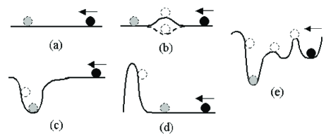
Figure 3: Sketch of possible subwalks of a particle. The solid dot, gray dot and open circle represent the initial position, finial position and some intermediate position of the particle, respectively; the arrow indicates the initial direction of the particle. (a) The particle moves and stops on a plateau. (b) The particle gets over a low potential barrier or a shallow well. (c) The particle stops in a deep well. (d) The particle rebounds on a high potential barrier. (e) The particle moves on a general landscape, and ends up in a deep well after many steps.

In the simulations, all $V_{i}$ start flat at time $t=0$, and are updated simultaneously at each time step $t(=1,2,\cdots)$, according to a rule to be specified below. But between two consecutive time steps, each walker moves a few steps in a subwalk in its own $V_{i}$, independent of other walkers. In a subwalk, the walker does not change $V_{i}$. The subwalk is like a particle rolling on a landscape with friction, with the following rules (with the subscript $i$ removed for the sake of clarity). The subwalk time is labeled by $\tau(=0,1,2,\cdots)$.
(i). At time $t=0$, the particle is arbitrarily placed on the $x$ axis.
(ii). At time $t$, the particle is given energy $K_{0}$ at $\tau=0$. ($K_{0}$ is a parameter fixed in the model.)
(iii). At subwalk time $\tau$, the particle moves left or right with equal probability. However, after each move, the particle loses energy $\varepsilon$, and the energy difference $V(x(\tau))-V(x(\tau+1))$ which could be positive or negative is added to its energy. Consequently, at time $\tau$, the particle already moves $\tau$ steps, and its energy becomes

$$K(\tau)=K_{0}+V_{0}-V(x(\tau))-\tau\varepsilon$$ (7)

where $V_{0}\equiv V(x(0))$, the potential at the initial position of the particle at $\tau=0$.
(iv). The particle can get over a potential barrier in $V$ that is lower than $K$, and can rebound if the barrier is higher than $K$.
(v). When the particle reaches the left boundary $(x=1)$ or the right boundary $(x=100)$, it reverses direction and continues its subwalk.
(vi). The particle stops when it walks into a potential well and cannot get out with its energy $K$, or exhausts its energy on a plateau.

These possibilities are sketched in FIG. 3. The reflecting boundary condition in item (v) corresponds to the real experimental situation where a dial with a limited range is used.

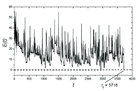
Figure 4: Dependence of the error function on time, from the eight-parameter AW model simulation.

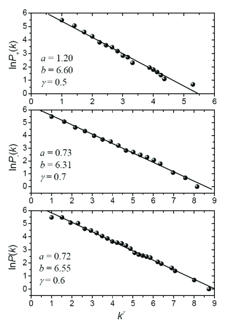
Figure 5: Numerical curves of $P_{+}(k)$, $P_{-}(k)$ and $P(k)$ obtained from the parameter-tuning networks from a eight-parameter AW model simulation, fitted to stretched exponent functions.

After all $N$ particles stop, the time clock increases from $t$ to $t+1$; the particle’s position at the end of its subwalk is taken to be $X(t+1)$, which is the starting position of the subwalk at time $t+1$. (The subwalks of the particles may not stop after the same number of subwalk steps; those stop first will sit there and wait for the last particle to stop.) The landscape $V_{i}(x_{i})$ is updated by the landscaping rule:

$$V_{i}(x_{i};t+1)=\left\{\begin{array}[]{cc}V_{i}(x_{i};t)+W(x_{i}-X_{i}(t+1)),\\ E(t)\geq E_{a}(t);\\ V_{i}(x_{i};t)-W(x_{i}-X_{i}(t+1)),\\ E(t)<E_{a}(t).\end{array}\right.$$ (8)

where $t=0,1,2,\cdots$. In our numerical simulations below, the ($i$-independent) landscaping function $W$ is given by $W(0)=4$, $W(\pm 1)=3$, $W(\pm 2)=1$, and $W=0$ otherwise. In Eq. (8), the error function $E(t)$ is assumed to be

$$E(t)=|Q(\emph{{u}}(t))-Q_{0}|$$ (9)

where $\emph{{u}}(t)$ is obtained from Eq. (6); $E_{a}(t)$ is the average error counting the last $n$ time steps, given by

$$E_{a}(t)=\frac{1}{n}\sum^{t}_{t^{\prime}=t-n+1}E(t^{\prime})$$ (10)

In computer simulations, we pretend that we know $Q_{0}$ and the $Q(\emph{{u}})$ function. In reality, the former is known to the experimenter; the latter can be roughly inferred from experimental data. Note that while the subwalks of the particles are independent of each other, the updating of their landscapes is affected by their collective effort through $Q(\emph{{u}})$ in $E(t)$.

The eight-parameter AW model is simulated with $t$ going from 0, and the simulation is stopped when the optimal parameter set is gotten. The function $Q$ is assumed to be

$$Q(\emph{{u}})=|u_{1}-10|+|u_{2}-10|+\cdots+|u_{8}-10|$$ (11)

The parameters used are: $K_{0}=23$, $\varepsilon=1$, $n=5$ and $Q_{0}=0$. This means that $\emph{{u}}=(10,10,\cdots,10)$ is the one and only optimal parameter set.

The error function $E(t)$ is displayed in FIG. 4, which shows that the optimal u is first obtained at $t_{0}=3718$. The 700 $\emph{{u}}(t)$ dots (with $300<t\leq 1000$, such number of $\emph{{u}}(t)$ is similar with the experimental data, and the initialization process when $t<300$ is ignored) in the u space are projected onto the $(u_{1},u_{2})$ plane to obtain the directed and non-directed networks. The corresponding cumulative degree distributions are given in FIG. 5. Good stretched-exponential fits are obtained, in agreement with the experimental findings in FIG. 2.

In the AW model, the subwalks kind of mimicking the action of the experimenter–we think that is why the AW model and the experiments give similar $P$ functions. Human dynamics Bar3 ; Vqz9 have been studied in other situations by different models. Our results imply that our network-based statistics and the AW model is helpful in the understanding of human action in the experimental processes and very likely in many other optimization projects. The stretched exponent property of the parameter-tuning network imply the human action in the optimization process could be having some quantitative principles, which is important for the experimental studies. Stretched exponent distributions or relations exist widely in many other systems XB4 ; Hol5 ; Sor1 ; Str1 . Since AW-like dynamics is very common in nature Lam2 , our model may reveal a new mechanism of stretched exponent distribution. By modifying the subwalks and tuning their parameters one may shorten $t_{0}$, the shortest time to find the optimal parameters, which would be of interest to the experimental researchers. Finally, the AW model mimics an optimization process in real experiment, could be useful in the optimization projects in many other systems.

We thank Lui Lam, Pin-Qun Jiang, Da-Ren He and Tao Zhou for useful discussions, and Sheng Liu, Shi-Hua Song, Jun Li and Yuan-Lai Xie for experimental help. This work is partially supported by China 973 Program (Grant No. 2006CB705500) and NSF China (Grant Nos. 60744003, 10635040, 10532060, 10472116, and 10575105).

References

- (1) D. J. Watts, S. H. Strogatz, Nature 393, 440 (1998).
- (2) A. -L. Barabási, R. Albert, Science 286, 509 (1999).
- (3) R. Albert, and A. -L. Barabási, Rev. Mod. Phys. 74, 47 (2002).
- (4) L. Lam, Int. J. Bifurcation & Chaos 15, 2317 (2005); Int. J. Bifurcation & Chaos 16, 239 (2006)
- (5) A. -L. Barabási, Nature 435, 207 (2005).
- (6) A. Vázquez, Phys. Rev. Lett. 95, 248701 (2005).
- (7) R. Xulvi-Brunet, and I. M. Sokolov, Phys. Rev. E 66, 026118 (2002).
- (8) A. J. Holanda, I. T. Pisa, O. Kinouchi, A. S. Martinez, and E. E. S. Ruiz, Physica A 344, 530 (2004).
- (9) J. Laherrère and D. Sornette, Eur. Phys. J. B 2, 525 (1998).
- (10) B. Sturman, E. Podivilov, and M. Gorkunov, Phys. Rev. Lett. 91, 176602 (2005).