Tectonic plate under a localized boundary
stress: fitting of a zero-range solvable model.
L. Petrova¹, B. Pavlov ^1,2.

¹ V.A.Fock Institute of Physics, St. Petersburg University, Russia.

² Department of Mathematics, the University of Auckland, New Zealand.

Abstract

We suggest a method of fitting of a zero-range model of a tectonic plate under a boundary stress on the basis of comparison of the theoretical formulae for the corresponding eigenfunctions/eigenvalues with the results extraction under monitoring, in the remote zone, of non-random (regular) oscillations of the Earth with periods 0.2-6 hours, on the background seismic process, in case of low seismic activity. Observations of changes of the characteristics of the oscillations (frequency, amplitude and polarization) in course of time, together with the theoretical analysis of the fitted model, would enable us to localize the stressed zone on the boundary of the plate and estimate the risk of a powerful earthquake at the zone.

Key-words Tectonic plate, Zero-range interaction, Operator extension

PACS numbers 91.45.D, 02.30.Jr, 02.30.Tb

1 Dynamics of the system of tectonic plates
and the motivation of the zero-range model.

The lithosphere of Earth consists of 14 tectonic plates which jigsaw fit each other. The plates are isolated from underlying solid structures within the Earth mantle by the low-viscosity layer of the asthenosphere which is formed, due to various conditions, including high pressure and temperature, in the interval of depth 100 -200 km. The plates move on the surface of Earth, due to convective flows and variations of the angular speed of Earth, gliding on the low-viscosity layer of asthenosphere and interacting with each other at some active boundary zones, see below.

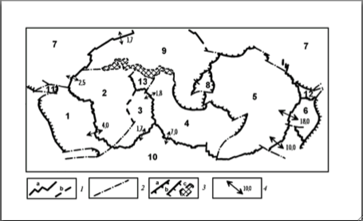
Figure 1:  

Boundaries of tectonic plates: 1- divergent boundaries (a - oceanic ridges, b- continental rifts), 2- transforming boundaries, 3-convergent boundaries (a-insular, b- active continental outskirts, c - collisions of plates). Directions and velocities of movement of plates ( cm/ year).

Fig. 1 below shows a complex form of boundaries between tectonic plates and their movements in different directions. The plates are enumerated in the following order : 1. South-American plate,   2. African plate ,   3. Somali plate,   4. Indian and Australian plates,   5. Pacific plate,   6. Nazca plate,   7. North-American plate,   8. Philippines plate,   9. Euro-Asian plate,   10. Antarctic plate,   11. Caribbean plate,   12. Cocos plate,   13. Arabian plate.

In addition to the 14 large plates described above there are 38 smaller plates (Okhotsk, Amur, Yangtze, Okinawa, Sunda, Burma, Molucca Sea, Banda Sea, Timor, Birds Head, Maoke, Caroline, Mariana, North Bismarck, Manus, South Bismarck, Solomon Sea, Woodlark, New Hebrides, Conway Reef, Balmoral Reef, Futuna, Niuafo’ou, Tonga, Kermadec, Rivera, Galapagos, Easter, Juan Fernandez, Panama, North Andes, Altiplano, Shetland, Scotia, Sandwich, Aegean Sea, Anatolia, Somalia), for a total of 52 plates.

It is commonly accepted that the tectonic plates are relatively thin elastic structures, approximately 100 km. thick, with linear size from 1000 km to several thousand km. The material of the plates, at the depth 100 km., has typical Young’s modulus 17.28 $\times$ 10¹⁰ kg  m^-1 sec^-2 , density 3380 kg m^-3 and Poisson coefficient 0.28. The velocity of the longitudinal waves in these materials is approximately 8000 m  sec^-1, and the velocity of the transversal (flexural) eigen-waves depends on the eigenvalues and varies, depending on the type of the wave, on a wide range around 4500 m  sec^-1, see the formula (4) below. Because of non accurate matching of the boundaries of the neighboring plates, the zones of direct contact of the plates are typically small- about 100 km.- compared with the linear size of the plates. Remaining inter-plate space is filled with loose materials, which are not able to accumulate any essential amount of elastic energy caused by the deformation. These materials can damp oscillations with short periods as 20 min. - 1 hour. Damping of acoustic waves by loose materials was discussed in [19, 11, 35]. Since tectonic plates are relatively thin, a major part of their kinetic energy is stored in the form of oscillatory flexural modes. The underlying layer of the asthenosphere makes flexural oscillation of plate possible, but also helps damping of the flexural waves with short periods, due to non-zero viscosity. Based on above data we conjecture that the flexural modes in different tectonic plates, in a certain range of periods, supposedly between $0.2h-1h$, see below the estimation of periods of eigen-modes of a model rectangular plate, are elastically disconnected from each other. Thus we expect that these flexural modes characterize elastic properties of the plates, but not the global elastic properties of the Earth’s crust.

The convective flows in the asthenosphere and variations of the angular speed of Earth, thanks to long-time variations of the moment of inertia of Earth, may cause collisions of neighboring plates. In presence of the liquid friction on the underlying layer of the asthenosphere, variations of the angular speed of earth cause mutual displacements of the neighboring plates, because small plates react immediately on the variations of the angular speed, and larger plates lag behind. These displacements cause collisions of the plates in the active zones, where the plates directly contact each other. Generally, when the angular speed of Earth decreases, with growing of the moment of inertia due to displacement of the center of gravity of Earth, the collisions may occur on the eastern boundaries of the major plates contacting smaller plates, observe, for instance, the contact of the Euro-Asia plate and the Philippines plate on Fig. 1. The stress caused by the collision may be either discharged due to forming cracks in the plates, splitting the active zone into independently moving fragments, or, being applied for an extended period of time, may cause accumulation of a considerable amount of (potential) elastic energy in the active zones of contacts, in form of elastic deformation of the stressed plates. This energy may be eventually discharged in form of a powerful earthquake.

Accumulation of the elastic energy, due to standard variational principle [7], causes the increment of eigenfrequencies of the tectonic plates. In [27, 32, 33] oscillatory processes, with similar spectral characteristics, were observed in mutually remote zones of the Euro-Asia plate. The authors of [27] suggested calling the processes seismo-gravitational oscillations of the Earth ( SGO). Recent analysis, based on data of the international GEOSCOPE network, revealed the existence of global oscillations with periods 3.97 h, 3.42 h, 1.03 h and 0.98 h. SGO with smaller periods do not have global character. They are usually observed in certain plates. For measurements of SGO, special devices are used (“vertical pendulum”), with high sensitivity to the variations of amplitudes and frequencies of SGO within the interval of periods 0.2 - 2 hours. Modification of the registering channel of the device allowed us to extend the interval to 0.2-6 hours. Results of analysis of measurements of SGO with relatively short periods from this range are presented in [30]. The data on SGO with longer periods and characteristics of modern 3-channel seismographs can be found in [29]. Observations with these devices reveal a wide spectrum of SGO. Some of the measured frequencies of SGO coincide with short-time variations of the angular speed of Earth, which were estimated based on astronomical observations, see the [28]. All experimental data confirm the presence of active energy in the system of tectonic plates, relevant to the inhomogeneity of the lithosphere.

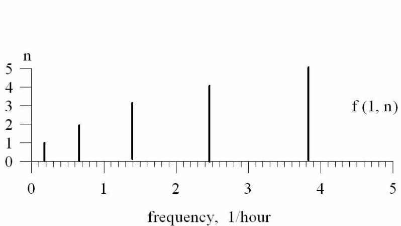
Figure 2:  

Computed eigenfrequencies of the rectangular plate 4 000 km $\times$ 8 000 km for the modes f(1, N)

Direct calculations of eigenfrequencies of the flexural modes of a rectangular thin plate $\Omega=d_{1}\times d_{2}$, $d_{1}=$ 4 000 km, $d_{2}=$ 8 000 km, 200 km thick, were done, see [21], based on bi-harmonic model, under natural assumptions concerning the density of the material is 3380 kg/m³, the Young’s modulus is 17.28 $\times$ 10¹⁰ $kg\,m^{-1}\,sec^{-2}$, and the Poisson coefficient is equal to 0.28. Though the Young’s modulus of a tectonic plate varies on a wide range of values, it is possible to provide a rough estimation, see below, of the periods of SGO and the length of the corresponding running waves of a tectonic plate, by computing these parameters for a model rectangular plate with elastic parameters equal to those of the tectonic plate on the half depth, 100 km. Indeed, the corresponding dynamical equation for the transversal (vertical) displacement $f$ is

$$\rho\frac{\partial^{2}f}{\partial t^{2}}+\frac{h^{2}\,E}{12(1-\sigma^{2})}\Delta^{2}f=0.$$ (1)

In [21] the simplest Neumann boundary conditions $\frac{\partial u}{\partial n}\bigg{|}_{\partial\Omega}=\frac{\partial\Delta u}{\partial n}\bigg{|}_{\partial\Omega}=0$ are imposed on the boundary. This allows us to solve the dynamical equation by Fourier method, via separation of variables. The eigenfunctions of the bi-harmonic operator coincide with the eigenfunction of the Neumann Laplacian, $f_{l_{1},l_{2}}=\cos\frac{\pi l_{1}x_{1}}{d_{1}}\cos\frac{\pi l_{2}x_{1}}{d_{2}}$, but the eigenvalues of the Neumann bi-harmonic operator

$$\lambda^{\Delta^{2}}_{l_{1},l_{2}}=\left[\lambda^{\Delta}_{l_{1},l_{2}}\right]^{2}=\left[\pi^{2}\left(l^{2}_{1}\,d_{1}^{-2}+l^{2}_{2}\,\,d_{2}^{-2}\right)\right]^{2}$$

are squares of the corresponding eigenvalues of the Neumann Laplacian. Taking into account that

$$\frac{h^{2}\,E}{12\rho(1-\sigma^{2})}=0.167\,\,10^{20}=\left[0.64\,\times 10^{5}\right]^{4}=:\alpha^{4},$$

we find the periods of flexural eigen-ocsillations from the formula:

$$\omega^{2}_{l_{1},l_{2}}=\left(\frac{2\pi}{T_{l_{1},l_{2}}}\right)^{2}=\alpha^{4}\,\left[\lambda^{\Delta}_{l_{1},l_{2}}\right]^{2},$$

or

$$\omega_{l_{1},l_{2}}=\frac{2\pi}{T_{l_{1},l_{2}}}=\alpha^{2}\,\,\,\lambda^{\Delta}_{l_{1},l_{2}}=:\alpha^{2}\,\,k^{2}_{l_{1},l_{2}},$$ (2)

where $k$ plays the role of the corresponding momentum. The speed of the transversal ( flexural) waves is calculated as

$$v^{f}_{l_{1},l_{2}}=\frac{\partial\Omega}{\partial k}=2\,\,\alpha\,\,k_{l_{1},l_{2}}.$$ (3)

Then for the above model plate the periods of flexural oscillations are defined by the formula $T_{hours}=2.63\,\,\,[4l_{1}^{2}+l_{2}^{2}]^{-1}\,\,\,hours$, and the velocity of the corresponding flexural waves are calculated as $v^{f}_{l_{1},l_{2}}=3400\sqrt{4l_{1}^{2}+l_{2}^{2}}\,\,\,m\,\,sec^{-1}$. In particular, the period of the flexural oscillation $f_{1,2}$ and the speed of the corresponding flexural wave $v^{f}_{1,2}$ are calculated as

$$T_{1,2}=0.33\,\,hours,\,\,\,v^{f}_{1,2}=9520\,\,m\,\,\sec^{-1},$$ (4)

and less for longer periods. The corresponding space-temporal oscillatory mode is

$$\cos{\omega_{1,2}t}\cos\frac{\pi\,x_{1}}{4000}\,\cos\frac{\pi\,2x_{2}}{8000},$$

with $x_{1},x_{2}$ measured in kilometers. This oscillatory mode can be represented as a linear combination of running flexural waves

$$\cos\left[\omega_{12}t\pm\frac{\pi\,x_{1}}{4000}\pm\frac{\pi\,x_{2}}{4000}\right].$$ (5)

The corresponding wavelength is estimated by the minimum of $\sqrt{\Lambda_{1}^{2}+\Lambda_{2}^{2}}$, where $\Lambda_{1},\Lambda_{2}$ correspond to the shift of the running wave by the corresponding period in time. For instance

$$\omega_{1,2}T_{12}=2\pi=\frac{\pi\,\Lambda_{1}+\pi\Lambda_{2}}{4000}$$

gives an estimation of the minimal wavelength as $\sqrt{\Lambda_{1}^{2}+\Lambda_{1}^{2}}\geq 5656$ km, which is much more than the diameter of the active zone, 5656 km $>>$ 100 km. Hence the zero-range model can be used, under above assumption, for the model stressed plate.

It appeared that periods of the eigen-modes $f_{1,1}-f_{5,5}$ sit in the interval 0.21 h - 5 h and their total number and distribution looks similar, see Fig. 2, to SGO described in the paper [27, 32, 33], despite the trivial plane rectangular geometry of the plate and trivial Neumann boundary conditions.

Examination of the results observed in [27, 32, 33] and theoretically obtained in [21] resulted in the conjecture that transversal SGO can be interpreted as flexural eigen-modes of the relatively thin tectonic plates. We hope that the zero-range model may be also used in this periods range for real tectonic plates as well.

In the next section we model dynamics of tectonic plates based on the bi-harmonic boundary problem with “natural” boundary conditions.

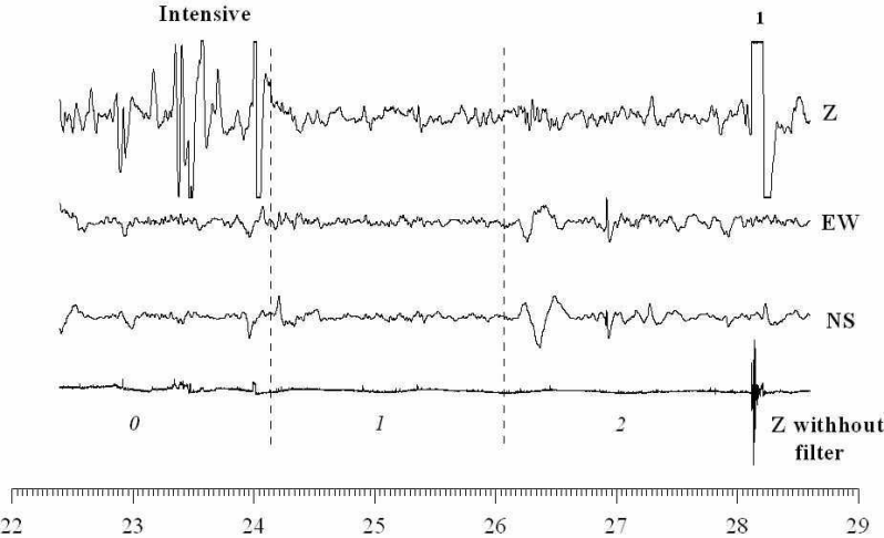
Figure 3: Dynamics of seismo-gravitational oscillations observed in St. Petersburg, 22-29 March 2000, see the text below.

Variation of the character of SGO is seen from comparison of the graphs of the amplitudes of SGO on 48-hours intervals of time separated by the vertical dotted lines. The graphs on these intervals show the reaction of the device on the oscillations of the ground.

A typical phenomenon of intense seismo-gravitational pulsation (SGP) was registered on the vertical component $Z$ on the initial interval marked by 0. This phenomenon was also noticed in the earlier paper [13]. See more about SPG in the further text, after the figure 4.

The components Z,EW and NS are obtained after filtration. The graph on the interval 1 shows the reaction of the filter on the maximal phase of the earthquake 28 March 2000 in Japan. The non-filtered graph Z represents the reaction of the base of the vertical seismograph on the transversal oscillations of the ground.

Spectral-time cards, see below fig. 4 represent the effect of growing of frequencies of SGO in visual form. The data of the observations were filtered by the band filter with the band strip [60 min.-300 min.]. We used the gliding time window length 700 min., and step-wise shifts with the 5 minutes steps. The interval of frequencies, measured in micro-Hertz, was chosen as $[70mcHz,250mcHz]=:[F_{min},F_{max}]$. For resolution $0.034mcHz$ the steps were halved to guarantee better smoothness of the spectral function.

Effect of growing of the frequency of SGO was detected only on spectral-time cards (ST-cards) of the vertical component of SGO, see below fig. 4. The frequencies are marked on the horizontal axes, time in hours - on the vertical axes, for the intervals 0,1,2 respectively. The level of spectral amplitudes is represented by the variation of the color. Oscillations with large spectral amplitudes, higher than the average level on the spectrum, are marked by grey color. The maximal amplitudes are marked by white color. The values of these amplitudes on the interval 0 are 3.5 times greater that the average amplitude, ( frequency about 200 mcHz). On the interval 1 they exceed the average amplitude in 1.8 times (the frequency about 200 mcHz). On the interval 2 they exceed the average amplitude in 3 times ( the frequency about 160 mcHz). For SGO with frequencies 90-110 mcHz and 170- 190 mcHz the amplitudes are 1.75 and 2.75 is times larger than the average amplitude. All three parts 0,1,2 of the fig. 4 reveal two patterns of inclined gray domains ( left-down to right-up and left-up to right-down) which correspond to SGO with growing and decreasing frequencies, correspondingly. This patterns provide an evidence of increment of the stored elastic energy in the system and discharging the stored elastic energy, respectively in form of oscillation modes with certain frequencies.

Growing of the frequency on the interval 2:

1. The frequency is growing from $f_{min}=80mcHz$ to $123mcHz$ during the period of 15 hours.

2. The frequency is growing from $f_{min}=130mcHz$ to $185mcHz$ during the period of 28.5 hours.

3.The frequency is growing from $f_{min}=170mcHz$ to $200mcHz$ during the period of 8 hours.

Growing of the frequency on the interval 0

1. The frequency is growing from $f_{min}=165mcHz$ to $205mcHz$ during the period of 33 hours.

2. The frequency is growing from $f_{min}=125mcHz$ to $165mcHz$ during the period of 15 hours.

Growing and decreasing of frequencies of SGO are easily noticeable also on the interval 1.

Growing of the frequency is characterized by the ratio $\frac{\Delta\nu}{\tau}$, where $\Delta\nu$ is the increment of the frequency and $\tau$ is the corresponding time interval, when the growing was observed.

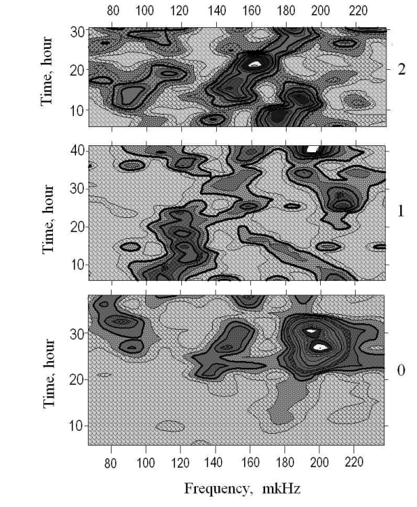
Figure 4: Time-frequency analysis of the vertical component of SGO

Other domains, where the frequency of the modes decrease with time growing, may be interpreted as an evidence of local relaxation of the stress, probably caused by local destruction of the plate (forming cracks).

We conjecture that the extended growth of frequencies of the SGO may be considered as a precursor of strong earthquakes. Our ability to extract useful information from the observations of frequencies and the shape of SGO is limited by our understanding of the mechanism of the variation of the frequency and the shape of SGO modes arising from the boundary stress on the tectonic plates.

There were also other observations of the shift of frequencies of selected modes of SGO. Note, that in numerous observations on SGO in Leningrad (St. Petersburg) intense short pulses were also recorded. They are constituted by several sinusoidal harmonics with periods from 30 minutes to 1 hour, and the total duration of the process 6- 10 hours. In several cases they were also followed by powerful earthquakes - in 2-4 days. This process was noticed first in [13] and was given the name of “seismo-gravitational pulsations”, SGP. Statistical analysis was done based on the data of the 6 months monitoring of SGO in St-Petersburg. This analysis confirmed that the connection between SGP and the subsequent strong earthquake is not random, with probability 95 %.

Essential information on SGO is obtained from the observation of variations of the frequencies and the shape of the corresponding modes in the remote zone. The typical size of the zone of contact is negligible - “point-wise”- when compared with the wavelength, which generally can be estimated as $\left[{\lambda}^{\Delta}\right]^{-1/2}$, see (5).

Although the boundaries of real tectonic plate are not smooth, however details of the local geometry of the boundaries may be neglected compared with the wavelength of typical waves on the plates. Then for SGO with periods 20 min. - 1 hour we may base the theoretical analysis of SGO on the bi-harmonic model for the relatively thin plate with natural boundary conditions. In this paper we also neglect presence of the liquid layer of the asthenosphere underlying the plate, thus reducing the problem to construction of self-adjoint extensions of the 2-d bi-harmonic operator.

In [31] we use the fact that characteristics of the seismo-gravitational oscillations in remote zone depend on a small number of basic parameters. On one hand, his fact is can be interpreted in a spirit of the Saint-Venant principle . On the other hand we were able to interpret this fact in the spirit of operator extensions. Based on this observation we developed in [31] a preliminary version of the above arguments and suggested to use a solvable zero-range model of the tectonic plates under a point-wise boundary stress, caused by the collision of plates. The role of the parameter of the model was played by some $3\times 3$ real Hermitian matrix $M$, see also next section. Thus the number of the Saint-Venant parameters for the boundary stressed relatively thin tectonic plate is 6. We presume, that the matrix $M$ defines the type of the stress, depending on mutual positions of the contacting plates at the active zone. There is a good reason to call $M$ the Saint-Venant matrix and the number of the Saint-Venant parameters (6) - the Saint-Venant number. We assume that mutual positions of the plates in active zone, and hence the matrix $M$ remains essentially unchanged during extended period. Thus the matrix $M$ characterizes the type of contact of tectonic plates in this location and remains the same for all earthquakes arising from the given active zone. In this paper, based on the compensation of singularities in the fundamental Krein formula, we suggest an explicit formula for the perturbed eigenfunctions of the plate. Comparison of the calculated eigenfunction with the data of the instrumental observations in remote zone, permits, in principle, to fit the model, that is, to find the basic matrix $M$. Once fitted, the constructed model would allow to calculate in explicit form the increment of the eigenvalues and the variations of the shape of the eigenfunctions of the stressed (perturbed) plate depending on the type and the magnitude of the local stress. We assume that the shifts of the eigenfrequencies and the changes of the shape of the eigen-modes can be measured for each active zone. With numerous active stations in the GEOSCOPE and IRIS networks, fitting of the proposed model can be done, eventually, for all active zones on the boundary of each major tectonic plate.

Generically earthquake hits only one active zone at a time. Then comparing the observed shift of the eigenfrequencies and the variations of the shape of the mode in the remote zone, where the Saint-Venant principle is applicable, with the results of computing based on the model, we will be able to localize the excited active zone based on the observed changes of the eigen-frequencies and the shapes (amplitude, polarization) of the flexural eigen-modes.

Mathematically the zero-range model of the isolated point-wise stressed tectonic plate and a similar zero-range model of the point-wise stressed tectonic plate submerged into environment formed by other plates, intermediate layers and asthenosphere, differ by the type of basic equations, but have a lot in common. In particular, the number of free parameters (6) for the point-wise active zone, in bi-harmonic model and Lame model is the same. We interpreted these parameters in the spirit of the Saint-Venant principle as essential parameters describing the shape of the wave-process in the remote zone, see [31]. In this paper we obtain the first order approximation for the perturbed eigenfrequencies and eigenfunctions based on a modified Krein formula, see [18, 1], for the point-wise stressed thin plate described by the bi-harmonic equation. The explicit representation of the perturbed eigen-modes permits to fit the zero-range model suggested in [31] based on results of instrumental measurements of SGO. We also conjecture that the properly fitted solvable model of the stressed tectonic plate may help to enlighten the nature of the pulsations.

2 Zero-range model of the point-wise boundary stress

We may base our approach on the standard mathematical model of the tectonic plate in form of a thin elastic plate, thickness $h$, with free edge, or on the 3-d Lame equations for displacements. We consider both options, describing in the next two subsections specific details of both models. Then we develop the common part of the theory, for both models simultaneously.

2.1 Thin plate model for the isolated tectonic
plate under the localized boundary stress

Denoting by $D$ the “the bending stiffness ”, connected with Young modulus $E$, the thickness $h$ of the plate and the Poisson coefficient $\sigma$ by the formula $D=Eh^{2}[12(1-\sigma^{2})]^{-1}$, we represent, following [12], the corresponding dynamical equation for the normal displacement $u$ as

$$\rho\frac{\partial^{2}u}{\partial s^{2}}=D\Delta^{2}u.$$

We consider time-periodic solutions $u(\omega s,\,x)$of the equation and separate the time, thereby reducing the dynamical problem to the spectral problem with the spectral parameter

$$\lambda=\rho D^{-1}\,\,\omega^{2}$$ (6)

for a bi-harmonic operator on a compact 2-d domain $\Omega$ - the tectonic plate - with a smooth boundary $\partial\Omega$:

$$Au=\Delta^{2}u=\lambda u,\,u\in W_{2}^{4}(\Omega),$$

and free boundary condition involving the tangential and normal derivatives of the displacement $u$ and the tension $\Delta u$:

$$\left[\frac{\partial\Delta u}{\partial n}+(1-\sigma)\frac{\partial^{3}u}{\partial n\partial t^{2}}\right]\bigg{|}_{\partial\Omega}=0,$$

$$\left[\Delta u-(1-\sigma)\frac{\partial^{2}u}{\partial t^{2}}\right]\bigg{|}_{\partial\Omega}=0.$$ (7)

Here $n,t$ are the normal and the tangent directions on the boundary.

The bi-harmonic operator $A$ is selfadjoint in the Hilbert space $L_{2}(\Omega):=\mathcal{H}$. The eigenfunctions of $A$ are smooth and they form an orthogonal basis in $L_{2}(\Omega)={\mathcal{H}}$. We consider the restriction $A_{0}$ of $A$ onto $D(A_{0})$ constituted by all smooth functions vanishing near the boundary point $a\in\partial\Omega$. The restriction is symmetric, but it is not selfadjoint, because the range of it $\left(A-{\lambda}I\right)D(A_{0})$, for complex $\Lambda$ has a nontrivial complement $N_{\lambda}$ which is a linear hull of the Green function $G(x,a,\bar{\lambda}):=g_{0}(x,\bar{\lambda})$ and its tangential derivatives $\frac{\partial G(x,a,\bar{\lambda})}{\partial t}:=g_{1}(x,\bar{\lambda}),\,\frac{\partial^{2}G(x,a,\bar{\lambda})}{\partial t^{2}}:=g_{2}(x,\bar{\lambda})$ of the first and second order, at the point $a$. The orthogonal complement $N_{\lambda}$ of the range is called the “deficiency subspace”, and elements of it - “deficiency elements”:

$$N_{\lambda}:={\mathcal{H}}\ominus(A_{0}-\lambda I)D_{0}=\bigvee_{s=0}^{2}g_{s}(*,\bar{\lambda}).$$

The deficiency elements have, at the boundary point $a$, singularities of different types ( see for instance [14], where much more general problem is considered) :

$$g_{0}(n,t)\approx(n^{2}+t^{2})\ln(n^{2}+t^{2}),\,\,g_{1}(n,t)\approx t\ln(n^{2}+t^{2}),\,\,g_{2}(n,t)\approx\ln(n^{2}+t^{2}),$$

hence they are linearly independent and form a basis in the deficiency subspace. The deficiency subspace at the spectral point $\bar{\lambda}$ is

$$N_{\bar{\lambda}}:={\mathcal{H}}\ominus(A_{0}-\bar{\lambda}I)D_{0}=\bigvee_{s=0}^{2}g_{s}{*,{\lambda}}.$$

The dimensions of the deficiency subspaces $(3,3)$ constitute the “deficiency index”. Hereafter we select $\lambda=i$ and attempt to construct a self-adjoint extension of $A_{0}$, which will play a role of a zero-range model of the tectonic plate under the boundary strain.

Note that Lame model the deficiency index is also $(3,3)$, on a smooth boundary. The role of deficiency elements is played by the columns of the Green matrix. The boundary of the tectonic plates may be assumed smooth for the long waves (small $\lambda$), since the integral shape of the solutions of the differential equations with small $\lambda$ is not affected by the details of the local geometry.

2.2 Construction of the self-adjoint extension

Extend $A_{0}$ from $D_{0}$ onto $D(A^{+}_{0})=D_{0}+N_{i}+N_{-}i$ as an “adjoint operator” $A^{+}_{0}$ by setting $\left(A^{+}_{0}\pm iI\right)g=0$ for $g\in N_{\mp i}$. This operator not selfadjoint, and it is not even symmetric, so that the boundary form

$$\langle A_{0}^{+}u,\,v\rangle-\langle u,\,A_{0}^{+}v\rangle={\mathcal{J}}(u,v)$$ (8)

does not vanish, generally, for $u,v\in D(A^{+}_{0})$. One can rewrite (8) in more convenient form with using new symplectic coordinates with respect of a new basis in $N$

$$W^{+}_{s}=\frac{1}{2}\left[g_{s}+\frac{A+iI}{A-iI}g_{s}\right]=\frac{A}{A-iI}g_{s}$$

$$W^{-}_{s}=\frac{1}{2i}\left[s_{s}-\frac{A+iI}{A-iI}g_{s}\right]=-\frac{I}{A-iI}g_{s}$$

Since $A_{0}^{+}g_{s}+ig_{s}=0,\,\,[A_{0}^{+}-iI]\frac{A+iI}{A-iI}g_{s}=0$ we have,

$$A_{0}^{+}W^{+}_{s}=W^{-}_{s},\,\,A_{0}^{+}W^{-}_{s}=-W^{+}_{s}.$$ (9)

Following [24] we will use the representation of elements from the domain of the adjoint operator, by the expansion on the new basis:

$$u=u_{0}+\sum_{s}\xi^{s}_{+}W^{+}_{s}+\xi^{s}_{-}W^{-}_{s}=u_{0}+\frac{A}{A-iI}\sum_{s}\xi^{s}_{+}g_{s}-\frac{I}{A-iI}\sum_{s}\xi^{s}_{-}g_{s}:=$$

$$=u_{0}+\frac{A}{A-iI}\vec{\xi}_{+}-\frac{I}{A-iI}\vec{\xi}_{-}.$$ (10)

Note that due to (9)

$$A^{+}\,\,\frac{A}{A-iI}\,\vec{\xi}_{+}=-\frac{I}{A-iI}\vec{\xi}_{+},\,\,A^{+}\,\frac{-I}{A-iI}\,\vec{\xi}_{-}=-\frac{A}{A-iI}\vec{\xi}_{-}.$$

Note that the boundary form

$$\langle A_{0}^{+}u,v\rangle-\langle u,A_{0}^{+}v\rangle:={\mathcal{J}}(u,v)$$

of elements $u,v$,

$$u=u_{0}+\frac{A}{A-iI}\vec{\xi}^{u}_{+}-\frac{I}{A-iI}\vec{\xi}^{u}_{-}:=u_{0}+n^{u},\,u_{0}\in D(A_{0})\,n^{u}\in N,$$ (11)

$$v=v_{0}+\frac{A}{A-iI}\vec{\xi}^{v}_{+}-\frac{I}{A-iI}\vec{\xi}^{v}_{-}:=v_{0}+n^{v},\,u_{0}\in D(A_{0})\,n^{v}\in N$$

depends only on components $n^{u},n^{v}$ of $u,v$ in the defect $N$. Then the boundary form is represented as:

$$\langle A_{0}^{+}u,v\rangle-\langle u,A_{0}^{+}v\rangle:={\mathcal{J}}(u,v)=\langle\vec{\xi}^{u}_{+},\vec{\xi}^{v}_{-}\rangle-\langle\vec{\xi}^{u}_{-},\vec{\xi}^{v}_{+}\rangle$$ (12)

with Euclidean dot-product for vectors $\vec{\xi}_{\pm}\in N_{i}$. Note that the representation of the boundary form in terms of abstract boundary values $\vec{\xi}_{\pm}$ contains only integral characteristics of the elements from the domain of the operators considered, and hence it is stable with respect of minor local perturbations of geometry of the plates. This enables us to substitute, for practical calculations, the real irregular boundaries of the plates by the smoothed boundaries, obtained via elimination of minor geometrical details, compared with the length of standing waves, circa 5000 km, of SGO with periods in the essential gange 20 min - 1 hour.

The boundary form vanishes on the Lagrangian plane defined in $D(A^{+}_{0})$ defined by the “boundary condition” with an Hermitian operator $M:N_{i}\to N_{i}$ :

$$\vec{\xi}_{+}=M\vec{\xi}_{-}.$$ (13)

This boundary condition defines a self-adjoint operator $A_{M}$ as a restriction of $A_{0}^{+}$ onto the Lagrangian plane ${\mathcal{T}}_{M}\in D(A_{0}^{+})$ defined by the boundary condition (13). The resolvent of $A_{M}$ defined by the boundary conditions is represented, at regular points of $A_{M}$, by the Krein formula, see [2, 24]:

$$\left(A_{M}-\lambda I\right)^{-1}=\frac{I}{A-\lambda I}-\frac{A+iI}{A-\lambda I}PM\frac{I}{I+P\frac{I+\lambda A}{A-\lambda I}PM}P\frac{A-iI}{A-\lambda I},$$ (14)

where $P$ is an orthogonal projection onto $N_{i}$.

2.3 Compensation of singularities in Krein formula
and calculation of the perturbed spectral data

Singularities of the resolvent $\left(A_{M}-\lambda I\right)^{-1}$ coincide with the spectrum of $A_{M}$. But both terms in the right side of (14) also have singularities on the spectrum of the non-perturbed operator $A$. The singularities of the first and second term the eigenvalues of $A$ compensate each other. We are able to derive this statement via straightforward calculation, in classical Krein-Birman-Schwinger formula and in the corresponding construction for quantum networks, see [18, 1]. In the course of the calculation of the compensation of singularities we can recover both the eigenvalues of the perturbed operator $A_{M}$ and the corresponding eigenfunctions, see [18]. Note that a similar statement, as a lemma on compensation of singularities of the corresponding Weyl-Titchmarsh function, was discovered in [6] for 1-d solvable model of the quantum network in form of a quantum graph. Later, in [16] and in [15], similar statements were proven for Dirichlet-to-Neumann maps of quantum networks. We formulate here this statement for the resolvent of the selfadjoint extension based on ideas proposed in [17].

We will observe the effect of compensation of singularities on a certain spectral interval $\Delta_{0}=[\lambda_{0}-\delta,\,\lambda_{0}+\delta]$, centered at the resonance eigenvalue $\lambda_{0}$ of the non-perturbed plate, assuming that the perturbation defined by the matrix $M$ is relatively small, in a certain sense, se below.

Assuming that there is a single eigenvalue $\lambda_{0}$ of $A$ on the interval $\Delta_{0}$, with the eigenfunction $\varphi_{0}$, we use the following representations, separating the polar terms from smooth operator functions $K_{i},K_{-1},K$ on $\Delta_{0}$

$$\frac{A+iI}{A-\lambda I}=(\lambda_{0}+i)\frac{\varphi_{0}\rangle\langle\varphi_{0}}{\lambda_{0}-\lambda}+K_{-i},$$

$$\frac{A-iI}{A-\lambda I}=(\lambda_{0}-i)\frac{\varphi_{0}\rangle\langle\varphi_{0}}{\lambda_{0}-\lambda}+K_{i},$$

$$P\frac{I+\lambda A}{A-\lambda I}P=(1+\lambda_{0}^{2})\frac{P\varphi_{0}\rangle\,\langle P\varphi_{0}}{\lambda_{0}-\lambda}+K(\lambda),$$ (15)

with a smooth matrix-function $K=K_{0}+o(|\lambda-\lambda_{0}|)$, with $K_{0}=K(\lambda_{0})$ and $\parallel o(|\lambda-\lambda_{0}|)\parallel\leq C_{0}\delta$.

Definition 2.1

We say that the matrix $M$ is relatively small, if $[I+K(\lambda)M]^{-1}$ exists and is bounded on $\Delta_{0}$.

This condition is obviously fulfilled if

$$\parallel[I+K(\lambda_{0})M]^{-1}\parallel\,C_{0}\delta<<1.$$ (16)

To calculate the second term in the right side of the Krein formula (14) we have to compute the inverse of the denominator, that is to solve the equation

$$\left[I+P\frac{I+\lambda A}{A-\lambda I}M\right]u=g$$ (17)

Though the standard analytic perturbation technique is still not applicable to this equation under the above conditions 2.1 or (16), we are able to construct the inverse based on finite dimensionality (one-dimensionality) of the polar term.

$$u=[I+KM]^{-1}g-(1+\lambda_{0}^{2})\frac{[I+KM]^{-1}P\varphi_{0}\rangle\langle P\varphi_{0}M[I+KM]^{-1}g\rangle}{\lambda_{0}-\lambda+\langle P\varphi_{0}M[I+KM]^{-1}\varphi_{0}\rangle}.$$ (18)

Based on (18) we are able, see [18, 1] to observe the compensation of singularities in the above Krein formula (14) and calculate the polar term of the resolvent at the single eigenvalue of the operator $A_{M}$ on the interval $\Delta_{0}$:

Theorem 2.1

If the perturbation is relatively small, as required in (2.1), then there exist a single eigenvalue $\lambda_{M}$ of the perturbed operator $A_{M}$ on the interval $\Delta_{0}$ which is found as a zero of the denominator in (18)

$$\lambda_{0}-\lambda+(1+\lambda_{0}^{2})\langle P\varphi_{0}M[I+KM]^{-1}\varphi_{0}\rangle:={\bf d}_{M}(\lambda),\,{\bf d}_{M}(\lambda_{M})=0$$ (19)

and the corresponding eigenfunction

$$\varphi_{M}=\varphi_{0}-(\lambda_{0}-i)K_{-i}M[I+KM]^{-1}P\varphi_{0},$$ (20)

computed at the zero $\lambda_{M}$. The polar term of the resolvent of the perturbed operator at the eigenvalue is represented as:

$$\frac{\varphi_{0}-(\lambda_{0}-i)K_{-i}M[I+KM]^{-1}P\varphi_{0}\rangle\langle\varphi_{0}-(\lambda_{0}-i)K_{-i}M[I+KM]^{-1}P\varphi_{0}}{{\bf d}_{M}(\lambda)}$$

Proof     of this statement can be obtained similarly to the corresponding statement in [18], where the case of several eigenvalues of the non-perturbed operator on an essential spectral interval was discussed. We consider here the simplest case, when only one eigenvalue of the unperturbed plate is present on an essential spectral interval. If the perturbation is small as required by the condition (16), then the approximate eigenvalue and the corresponding approximate eigenfunction of $A_{M}$ can be obtained via replacement $K,K_{\pm i}$ in (19,20) by $K(\lambda_{0}),K_{\pm i}(\lambda_{0})$:

$$\lambda_{M}\approx\lambda_{0}+(1+\lambda_{0}^{2})\langle P\varphi_{0}M[I+K(\lambda_{0})M]^{-1}K(\lambda_{0})\varphi_{0}\rangle,$$

$$\varphi_{M}\approx\varphi_{0}-(\lambda_{0}-i)K_{-i}(\lambda_{0})M[I+K(\lambda_{0})M]^{-1}P\varphi_{0}.$$ (21)

Remark Analysis of the multi-point boundary condition which corresponds to several stresses applied at the points $a_{1},a_{2},\dots a_{m}$ on the boundary of the plate $\Omega$ differs from the above analysis of the single-point case, only in the first step. In the case of a multi-point stress we have to construct of elements $\left\{g_{0}^{r}(x,a_{r},i),\,g_{1}^{r}(x,a_{r},i),\,g_{2}^{r}(x,a_{r},i)\right\}_{r=1}^{m}$ a basis in the larger deficiency subspace $N_{i}$,  dim $N_{i}=3m$. Due to the presence of singularities of different types at different points, the deficiency elements are linearly independent.

3 Concluding remarks on the fitting
of the model

The pair of data (2.3) may be used in two different ways: either for calculation of the shift of the frequency of SGO and the corresponding perturbation of the eigenfunction, under the point-wise stress characterized by the matrix $M$, or, vice versa, for recovering of the data on the localization, the type and the intensity of the stress from instrumental observations.

Indeed, if the geological structure of the tectonic plates at the active zones, encoded in matrices $M_{s}$ attached to the zones, are known, then, theoretically, we are able to calculate the eigenfunctions and the eigenfrequencies of the plates, taking into account the stress caused by collisions. We are also able, theoretically, to construct the deficiency elements for all active zones. Then the self-adjoint extension of the bi-harmonic operator on the plate, with the point-wise boundary stress, can be constructed, with the corresponding matrices $M_{s}$. The obtained theoretical results can be compared with the results of the instrumental measurements. This permits to recover the matrices $M_{s}$, which characterize the stressed points $a_{1},\,a_{2},\,\dots$.

Assume that the structure of the plates at the collision point $a$ remains unchanged, but the tension is growing linearly with time $\tau$ as: $M(\tau)=m\tau$, with a matrix coefficient $m:N\to N$. Then the formulae (20,19), for small $\tau$, define the derivatives of $\lambda_{M},\varphi_{M}$ with respect to $\tau$ at the moment $\tau=0$:

$$\frac{\partial\varphi_{M}}{\partial\tau}\bigg{|}_{\tau=0}=-(\lambda_{0}-i)K_{-i}m_{0}P_{+}\varphi_{0}(x_{s}),\,\,\,\frac{\partial\lambda_{M}}{\partial\tau}\bigg{|}_{\tau=0}=(1+\lambda^{2}_{0})\langle P_{+}\varphi_{0},m\,\,P_{+}\varphi_{0}\rangle.$$

Comparing this result with ratios

$$\frac{\varphi_{m\tau}(x_{s})-\varphi_{0}}{\tau}(x_{s})\bigg{|}_{\tau=0},\,\,\frac{\lambda_{m\tau}-\lambda_{0}}{\tau}\bigg{|}_{\tau=0},$$

measured experimentally for the amplitude and frequency of SGO, we are able to find fit $m$, and calculate the increment of $M$ $\delta M=\tau m$.

Practical experience in analytic perturbations shows, that minor perturbations affect rather the eigenvalues, than the the shapes of the eigenfunctions of the spectral problem. Based on this observation we can estimate the speed of accumulation of elastic energy $\mathcal{E}$, under the point-wise boundary stress depending on the speed of the shift of the eigenvalues (eigenfrequencies) of SGO and initial distribution of the elastic energy on the modes $\varphi^{s}_{0}$ defined by the corresponding Fourier coefficients $\langle u,\varphi^{s}_{0}\rangle$:

$$\frac{d{\mathcal{E}}}{d\tau}\approx\sum_{s}\frac{d\lambda_{M}^{s}}{d\tau}|\langle u,\varphi^{s}_{0}\rangle|^{2}=\sum_{s}(1+(\lambda^{s})^{2}_{0})\langle P_{+}\varphi^{s}_{0},m\,\,P_{+}\varphi^{s}_{0}\rangle\,\,|\langle u,\varphi^{s}_{0}\rangle|^{2},$$

with the summation extended only on the eigen-modes which correspond to the varying eigenvalues. If only one active zone $a_{s}$ is involved at a time, then only one matrix $M_{s}$ has to be taken into account, so that the risk of the powerful earthquake may be estimated based on the magnitude of $\delta_{s}=\tau m_{s}$.

If there are several active zones at the points $a_{1},a_{2},\dots a_{n}$ on the boundary of the plate, then the corresponding matrices $M_{1},M_{2},\dots M_{n}$ can be fitted based on observations of SGO in the remote zone during preceding earthquakes which occurred at $a_{1},a_{2},\dots a_{n}$. Variations of the frequencies and the shape of SGO may arise from the stress at any active zone, but usually only one active zone is involved at a time. Once the matrices $M_{1},M_{2},\dots$ are known, then comparison of the perturbation of the frequencies and the shapes of seismo-gravitational modes, SGM (or, probably, seismo-gravitational pulsations, SGP) at the given groups of points in the remote zone with results of previous measurements at these points, would allow us to identify the active zone where the stress is applied. We presume that the above model gives a chance to introduce a useful system into the scope of the experimental data on the seismo-gravitational oscillations in remote zone and use them for estimating of risk and localization of the powerful earthquakes. This opens an alternative to the statistical methods, see [34], of estimation of risk of powerful earthquakes.

Fitting of the proposed model in reality requires both extended computing and a major experimental data base. Because the wavelengths of the standing waves, circa 5000 km, on the essential range of periods, 20 min- 1 hour,dominate the size of the active zones, one may assume, that the straightforward computing with averaged and smoothed data for Young’s modulus and geometric characteristics of the plates will enables us to obtain a realistic approximation of the deficiency elements, with singularities at the active zones, and to construct the perturbed eigenfunctions of the plates, which correspond to SGO.

More accurate theory requires taking into account realistic boundary conditions, and the exchange of energy with the liquid underlay and neighboring plates. In particular, arising new modes in the spectrum of SGO of the plate, transferred, due to the tight contact in active zone, from the neighboring plate may be considered as another possible precursor of a powerful earthquake. The choice of realistic boundary conditions has to be done based on experimental data interpreted within an appropriate extension of the scheme proposed above, with Lame and hydro-dynamical equations involved. We postpone discussion of these interesting questions to oncoming publications.

4 Acknowledgement

The initial version of the text was presented at the I.G.Petrovskii conference Moscow, May 21-26, 2007, see [26], and issued as a preprint of the Semester of Quantum Graphs at the International Newton institute, Cambridge, January - June 2007, see [22]. The authors acknowledge support from the organizers and participants of these meetings. The authors are grateful to Doctor Colin Fox for an inspiring discussion of the Saint-Venant principle. L. Petrova acknowledges support from the RFFI grant 01-05-64753, B. Pavlov acknowledges support from the grant of the Russian Academy of Sciences, RFFI 97-01-01149.

References

- [1] V.Adamyan, B. Pavlov, A. Yafyasov Modified Krein formula and analytic perturbation procedure for scattering on arbitrary junction Preprint of the International Newton Institute, NI07016, 18th April 2007, 30 p.
- [2] N.I.Akhiezer, I.M.Glazman, Theory of Linear Operators in Hilbert Space, (Frederick Ungar, Publ., New-York, vol. 1, 1966) (Translated from Russian by M. Nestel)
- [3] S.V.Aplonov Geodinamika. Published by Sankt-Petersburg University (In Russian) 2001, 360 p.
- [4] S.Albeverio, P.Kurasov, Singular perturbations of differential operators. Solvable Schrödinger type operators. London Mathematical Society Lecture Note Series, 271. Cambridge University Press, Cambridge, 2000. xiv+429 pp
- [5] F.A.Berezin, L.D. Faddeev A remark on Schrödinger equation with a singular potential Soviet Math. Dokl. 2 (1961) pp. 372-376.
- [6] V.Bogevolnov, A.Mikhailova, B. Pavlov, A.Yafyasov About Scattering on the Ring In: ”Operator Theory : Advances and Applications”, Vol 124 (Israel Gohberg Anniversary Volume), Ed. A. Dijksma, A.M.Kaashoek, A.C.M.Ran, Birkhäuser, Basel (2001) pp. 155-187
- [7] Courant, R.; Hilbert, D. Methoden der mathematischen Physik. I. (German) Dritte Auflage. Heidelberger Taschenb cher, Band 30. Springer-Verlag, Berlin-New York, 1968. xv+469 p.
- [8] Yu.N.Demkov, V.N.Ostrovskij, Zero-range potentials and their applications in Atomic Physics, Plenum Press, NY-London (1988).
- [9] E.Fermi Sul motto dei neutroni nelle sostance idrogenate (in Italian) Ricerca Scientifica 7(1936) p 13 .
- [10] Yu.E.Karpeshina, B. S. Pavlov Interactions of the zero radius for the bi-harmonic and the poly-harmonic equations , (in Russian). Mat. Zametki, 40 (1986), no 1, 49-59, 140. (English translation: Math. Notes 40 (1987) , no 1-2, 528-533).
- [11] Y. A. Kupertin On acoustic properties of vibration protection of the reactor PIK (In Russian), Preprint of Leningrad Institute of Nuclear Physics, Gatchina (1979), 23 p
- [12] L.D. Landau, E.M. Lifschitz, Lehrbuch der theoretischen Physik (”Landau-Lifschitz”). Band VII. (German) [Textbook of theoretical physics (”Landau-Lifschitz”). Vol. VII] Elastizit tstheorie. [Elasticity theory] Translated from the Russian by Benjamin Kozik and Wolfgang G hler. Seventh edition. Akademie-Verlag, Berlin (1991) 223 p.
- [13] E.M. Lin’kov, L.N. Petrova, K.S.Osipov Seismogravitational pulsations of the Earth and Atmospheric perturbations as possible Precursors to strong earthquakes. Translations: Doklady of the USSR Academy of Sciences: Earth Science Section, 313 (1992) pp. 76-79.
- [14] V.G.Mazja, B.A.Plamenevskii The coefficients in the asymptotic form of the solution of elliptic boundary value problem in domains with conical points Mathematische Nachrichten,76 (1977) pp 29-60.
- [15] A. Mikhailova, B. Pavlov Resonance Quantum Switch In : S.Albeverio, N.Elander, W.N.Everitt and P.Kurasov (eds.), Operator Methods in Ordinary and Partial Differential Equations. S.Kovalevski Symposium,132, Univ. of Stockholm, June 2000 , Birkhauser, Basel-Boston-Berlin, (2002) pp 287-322.
- [16] A. Mikhailova, B. Pavlov Quantum Domain as a triadic Relay In: Unconventional models of Computations UMC’2K, ed. I. Antoniou, C. Calude, M.J. Dinneen, Springer Verlag series for Discrete Mathematics and Theoretical Computer Science (2001) pp 167-186
- [17] A. Mikhailova, B. Pavlov, L.Prokhorov Modelling of Quantum Networks arXiv math-ph/031238, 2004, 69 p.
-
[18]
A. Mikhailova, B. Pavlov Remark on compensation of
singularities in Krein formula. Accepted by: Operator theory: Advances and applications, Proceedings of OTAMP06, ed. P. Kurasov, A.Laptev, S. Naboko, Lund, June 2006, 9 p. - [19] R.I.Nigmatulin Foundations of the mecchanics of heterogeneous media (In Russian) Nauka, Moscow (1978) 336 p.
- [20] John von Neumann Mathematical foundations of quantum mechanics. Translated from the German and with a preface by Robert T. Beyer. Twelfth printing. Princeton Landmarks in Mathematics. Princeton Paperbacks. Princeton University Press, Princeton, NJ, 1996. xii+445 pp.
- [21] K.S.Osipov Adaptive analysis of the non-stationary time series in study of seismic oscillations with periods 0.5-5 hours, (in Russian). PhD thesis, Sankt-Petersburg University, (1992) 110 p.
-
[22]
B. Pavlov, L.Petrova The problem of fitting of
the zero-range
model of the tectonic plate under a localized boundary stress International Newton Institute report series NI 07027, Cambridge, 30 April, 2007, 19 p. - [23] B. Pavlov, V. Kruglov Operator Extension technique for resonance scattering of neutrons by nuclei In: Hadronic Journal 28, June 2005, pp 259-268.
- [24] B. Pavlov The theory of extensions and explicitly-solvable models Russian Math. Surveys 42,6 (1987) pp 127-168.
- [25] B.Pavlov A star-graph model via operator extension Mathematical Proceedings of the Cambridge Philosophical Society, Volume 142, Issue 02, March 2007, pp 365-384 .
- [26] B.Pavlov Saint-Venant principle and an explicitly-solvable model of a thin plate under a pointwise boundary stress. International Conference “Differential Equations and related Topics” ( dedicated to I.G. Petrovskii), May 21-26, Moscow. Book of abstracts, p. 236.
- [27] L.N.Petrova, E.M.Lin’kov,D.D. Zuroshvili Planetary character of superlong oscillations of earth (In Russian) Vestnik LGU, ser.4, vyp. 4(25) (1988), pp 21-26.
- [28] L.N.Petrova, D.V. Lybimtsev Global Nature of the Sesmogravitational Oscillations of the Earth . Izvestiya, Physics of the Solid Earth, 42,(2), 114-123 (2006).
- [29] L.N.Petrova, E.G. Orlov,V.V. Karpinsky On dynamics and structure of oscillations of Earth in December 2004 according to observations on seismogravimeter in St. Petersburg. Izvestiya, Physics of the Solid Earth, 43,(2), 111-118 (2007).
- [30] L.N.Petrova Oscillations of the Earth with Periods from 9 min to 57 min in the Background Seismic Process and the Energy Flux Direction in the range of the free oscillation . To appear in: Izvestiya, Physics of the Solid Earth, 44,(1), 1-14 (2008).
- [31] L.N.Petrova, B.S.Pavlov, L.S.Ivlev On the issue of seismographical oscillations of Earth: perturbation of eigenfrequencies of a thin plate under a pointwise boundary strain. (In Russian). Submitted to Proceedings of the inter-regional conference ”Ekologiya i kosmos - 2007 ”. Sankt-Petersburg University (2008)
- [32] L.N. Petrova The seismic process in the frequency range 0.05-0.5 mHz: Patterns and Peculiarities..Volc. Seis., 2000, vol.21, 573-585
- [33] Petrova L.N. Seismogravitational Oscillations of the Earth from Observations by Spaced Vertical Pendulums in Eurasia.Izvestiya, Physics of the Solid Earth. Vol.38, No 4, 2002, 325-336.
- [34] W. Smith (GNS Science Lower Hutt, New Zealand) Earthquake risk assessment: from scientific research to risk management decisions. Science and security. Conference of RSNZ, Wellington, 17 November 2005. SESSION 2
- [35] Xiaofan Li Scattering of seismic waves in arbitrarily heterogeneous and acoustic media: A general solution and simulations GEOPHYSICAL RESEARCH LETTERS, 28,15,(2001) pp 3003 3006