APPROXIMATE JOINT MEASURABILITY OF SPIN ALONG TWO DIRECTIONS

Teiko Heinosaari, Peter Stano, and Daniel Reitzner Research Center for Quantum Information, Slovak Academy of Sciences, DΓΊbravskΓ‘ cesta 9, 845 11 Bratislava, Slovakia temihe@utu.fi; peter.stano@savba.sk; daniel.reitzner@savba.sk
Abstract.

We study the existence of jointly measurable POVM approximations to two non-commuting sharp spin observables. We compare two different ways to specify optimal approximations.

1. Introduction

Joint measurability for sharp observables is equivalent to the commutativity of the corresponding selfadjoint operators. The question that we study here is the following: having two non-commuting sharp spin observables (which are thus not jointly measurable), what is the closest approximation, in the form of two positive operator valued measures (POVMs), such that these two POVMs are jointly measurable. We show when such approximations exist as regions of allowed points in a suitably chosen space of parameters. This approach allows us, for example, to quantify how far we have to go from the original sharp observables to get jointly measurable approximations. Futhermore, optimal approximations can be identified as those laying on the boundary of such regions.

2. Statement of the problem

Let 𝒫𝒫\mathcal{P} and 𝒬𝒬\mathcal{Q} be two observables corresponding to sharp measurements of spin in the directions 𝐩𝐩\mathbf{p} and πͺπͺ\mathbf{q}, respectively. They are described by selfadjoint operators Οƒπ©β‰‘π©β‹…πˆsubscriptπœŽπ©β‹…π©πˆ\sigma_{\mathbf{p}}\equiv\mathbf{p}\cdot\boldsymbol{\sigma} and Οƒπͺ≑πͺβ‹…πˆsubscript𝜎πͺβ‹…πͺ𝝈\sigma_{\mathbf{q}}\equiv\mathbf{q}\cdot\boldsymbol{\sigma}, with ‖𝐩‖=β€–πͺβ€–=1norm𝐩normπͺ1\left\|\mathbf{p}\right\|=\left\|\mathbf{q}\right\|=1. Alternatively, and for our purposes more conveniently, these observables can be described by two outcome PVMs (projection valued measures). Then 𝒫𝒫\mathcal{P} is described by a mapping 1↦Pmaps-to1𝑃1\mapsto P, βˆ’1↦Iβˆ’Pmaps-to1𝐼𝑃-1\mapsto I-P with P𝑃P being the projection P=12​(I+π©β‹…πˆ)𝑃12πΌβ‹…π©πˆP=\tfrac{1}{2}(I+\mathbf{p}\cdot\boldsymbol{\sigma}), and 𝒬𝒬\mathcal{Q} is similarly described by a PVM corresponding to projections Q=12​(I+πͺβ‹…πˆ)𝑄12𝐼⋅πͺ𝝈Q=\tfrac{1}{2}(I+\mathbf{q}\cdot\boldsymbol{\sigma}) and Iβˆ’Q𝐼𝑄I-Q. We denote by ΞΈπœƒ\theta the angle between 𝐩𝐩\mathbf{p} and πͺπͺ\mathbf{q} and we assume that 0<θ≀90∘0πœƒsuperscript900<\theta\leq 90^{\circ}.

A joint measurement for 𝒫𝒫\mathcal{P} and 𝒬𝒬\mathcal{Q} is defined as a measurement with four outcomes corresponding to four possible pairs of 𝒫𝒫\mathcal{P} and 𝒬𝒬\mathcal{Q} outcomes, (Β±1,Β±1)plus-or-minus1plus-or-minus1(\pm 1,\pm 1). In addition, it is required that the measurement outcome statistics for 𝒫𝒫\mathcal{P} (𝒬𝒬\mathcal{Q}) measured alone can be obtained from the joint measurement by disregarding (summing through all possible) outcomes for 𝒬𝒬\mathcal{Q} (𝒫𝒫\mathcal{P}). Thus, 𝒫𝒫\mathcal{P} and 𝒬𝒬\mathcal{Q} are jointly measurable if there exist four operators G++,G+βˆ’,Gβˆ’+,Gβˆ’βˆ’subscript𝐺absentsubscript𝐺absentsubscript𝐺absentsubscript𝐺absentG_{++},G_{+-},G_{-+},G_{--} such that

(1) P=G+++G+βˆ’,Q=G+++Gβˆ’+.formulae-sequence𝑃subscript𝐺absentsubscript𝐺absent𝑄subscript𝐺absentsubscript𝐺absentP=G_{++}+G_{+-}\,,\quad Q=G_{++}+G_{-+}\,.

These operators must form a POVM, hence they are positive and satisfy βˆ‘i​jGi​j=Isubscript𝑖𝑗subscript𝐺𝑖𝑗𝐼\sum_{ij}G_{ij}=I. It is well known that 𝒫𝒫\mathcal{P} and 𝒬𝒬\mathcal{Q} are jointly measurable if and only if P𝑃P and Q𝑄Q commute, which is the case when 𝐩=Β±πͺ𝐩plus-or-minusπͺ\mathbf{p}=\pm\mathbf{q}. Thus, if 𝐩≠±πͺ𝐩plus-or-minusπͺ\mathbf{p}\neq\pm\mathbf{q}, a joint measurement can only approximate 𝒫𝒫\mathcal{P} and 𝒬𝒬\mathcal{Q}.

We are looking for observables π’œπ’œ\mathcal{A} and ℬℬ\mathcal{B} such that they are jointly measurable and can be taken as approximations to 𝒫𝒫\mathcal{P} and 𝒬𝒬\mathcal{Q}. An observable π’œπ’œ\mathcal{A} with two outcomes Β±1plus-or-minus1\pm 1 is described by a POVM 1↦Amaps-to1𝐴1\mapsto A, βˆ’1↦Iβˆ’Amaps-to1𝐼𝐴-1\mapsto I-A, where A𝐴A is an operator on β„‚2superscriptβ„‚2\mathbb{C}^{2} satisfying O≀A≀I𝑂𝐴𝐼O\leq A\leq I. It can be parametrized by four real parameters,

(2) A=12​(α​I+πšβ‹…πˆ),β€–πšβ€–β‰€Ξ±β‰€2βˆ’β€–πšβ€–.formulae-sequence𝐴12π›ΌπΌβ‹…πšπˆnormπšπ›Ό2norm𝐚A=\frac{1}{2}(\alpha I+\mathbf{a}\cdot\boldsymbol{\sigma}),\quad\left\|\mathbf{a}\right\|\leq\alpha\leq 2-\left\|\mathbf{a}\right\|\,.

If Ξ±=1𝛼1\alpha=1, then the condition in (2) reduces to β€–πšβ€–β‰€1norm𝐚1\left\|\mathbf{a}\right\|\leq 1. In a similar way, ℬℬ\mathcal{B} is described by a POVM corresponding to operator B=12​(β​I+π›β‹…πˆ)𝐡12π›½πΌβ‹…π›πˆB=\tfrac{1}{2}(\beta I+\mathbf{b}\cdot\boldsymbol{\sigma}) with ‖𝐛‖≀β≀2βˆ’β€–π›β€–norm𝐛𝛽2norm𝐛\left\|\mathbf{b}\right\|\leq\beta\leq 2-\left\|\mathbf{b}\right\|.

For sharp observables joint measurability is equivalent to commutativity. The decision whether two observables are jointly measurable is, however, more involved for observables in general. A general characterization of joint measurability of π’œπ’œ\mathcal{A} and ℬℬ\mathcal{B} is, up to authors knowledge, an open problem. However, for the task under consideration the following result [1] of Busch will be enough: if Ξ±=Ξ²=1𝛼𝛽1\alpha=\beta=1, then the necessary and sufficient condition for π’œπ’œ\mathcal{A} and ℬℬ\mathcal{B} to be jointly measurable is

(3) β€–πšβˆ’π›β€–+β€–πš+𝐛‖≀2.normπšπ›normπšπ›2\left\|\mathbf{a}-\mathbf{b}\right\|+\left\|\mathbf{a}+\mathbf{b}\right\|\leq 2\,.

If α𝛼\alpha and β𝛽\beta are not equal to 1, this condition is still necessary for joint measurability [2].

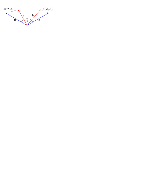
We will quantify how well π’œπ’œ\mathcal{A} approximates 𝒫𝒫\mathcal{P} using two different distances d​(𝒫,π’œ)π‘‘π’«π’œd(\mathcal{P},\mathcal{A}) in the next sections. We then solve the following problem: for a fixed distance111Observable π’œπ’œ\mathcal{A} is not fixed - we allow all π’œπ’œ\mathcal{A} which have the fixed distance from 𝒫𝒫\mathcal{P}. d​(𝒫,π’œ)π‘‘π’«π’œd(\mathcal{P},\mathcal{A}), find the smallest possible distance d​(𝒬,ℬ)𝑑𝒬ℬd(\mathcal{Q},\mathcal{B}) such that π’œπ’œ\mathcal{A} and ℬℬ\mathcal{B} are jointly measurable. The task is summarized in Fig.Β 1.

Refer to caption

Figure 1. The observables 𝒫𝒫\mathcal{P} and 𝒬𝒬\mathcal{Q} are parametrized by unit vectors 𝐩𝐩\mathbf{p} and πͺπͺ\mathbf{q} making an angle ΞΈπœƒ\theta. Two jointly measurable POVM approximations π’œπ’œ\mathcal{A} and ℬℬ\mathcal{B} are parametrized by vectors 𝐚𝐚\mathbf{a} and 𝐛𝐛\mathbf{b}. The smaller is the distance d​(𝒫,π’œ)π‘‘π’«π’œd(\mathcal{P},\mathcal{A}), the better π’œπ’œ\mathcal{A} approximates 𝒫𝒫\mathcal{P}.

3. Statistical distance

One possible way to quantify the distance between π’œπ’œ\mathcal{A} and 𝒫𝒫\mathcal{P} is to compare the probabilities that these observables give for states. There are at least two reasonable choices: we can calculate the worst possible deviation or the average deviation between the probability distributions on the outcomes. For the worst possible deviation we get

(4) supΟβ€‹βˆ£tr​[ρ​P]βˆ’tr​[ρ​A]∣=12β€‹β€–π©βˆ’πšβ€–+12​|1βˆ’Ξ±|.subscriptsup𝜌delimited-∣∣trdelimited-[]πœŒπ‘ƒtrdelimited-[]𝜌𝐴12norm𝐩𝐚121𝛼\textrm{sup}_{\rho}\mid\textrm{tr}\left[\rho P\right]-\textrm{tr}\left[\rho A\right]\mid=\tfrac{1}{2}\left\|\mathbf{p}-\mathbf{a}\right\|+\tfrac{1}{2}|1-\alpha|\,.

On the other hand, the average deviation can be calculated using pure states ψ𝐫subscriptπœ“π«\psi_{\mathbf{r}} parametrized by the points 𝐫𝐫\mathbf{r} in the unit sphere in ℝ3superscriptℝ3\mathbb{R}^{3}, and we get222For 𝐩=𝐚𝐩𝐚\mathbf{p}=\mathbf{a} the right hand side of (5) is 12​|1βˆ’Ξ±|121𝛼\tfrac{1}{2}|1-\alpha| and the following analysis still holds.

(5) 14β€‹Ο€β€‹βˆ«π«βˆˆS2∣⟨ψ𝐫|Pβ€‹Οˆπ«βŸ©βˆ’βŸ¨Οˆπ«|Aβ€‹Οˆπ«βŸ©βˆ£β€‹π‘‘π«=14β€‹β€–π©βˆ’πšβ€–+(1βˆ’Ξ±)24β€‹β€–π©βˆ’πšβ€–.14πœ‹subscript𝐫superscript𝑆2delimited-∣∣inner-productsubscriptπœ“π«π‘ƒsubscriptπœ“π«inner-productsubscriptπœ“π«π΄subscriptπœ“π«differential-d𝐫14norm𝐩𝐚superscript1𝛼24norm𝐩𝐚\frac{1}{4\pi}\int_{\mathbf{r}\in S^{2}}\mid\left\langle\,\psi_{\mathbf{r}}\,|\,P\psi_{\mathbf{r}}\,\right\rangle-\left\langle\,\psi_{\mathbf{r}}\,|\,A\psi_{\mathbf{r}}\,\right\rangle\mid d\mathbf{r}=\frac{1}{4}\left\|\mathbf{p}-\mathbf{a}\right\|+\frac{(1-\alpha)^{2}}{4\left\|\mathbf{p}-\mathbf{a}\right\|}\,.

Clearly, in both cases the choice Ξ±=1𝛼1\alpha=1 makes the distance smallest independently on 𝐚𝐚\mathbf{a}. Moreover, as shown in Ref.Β [2] the joint measurability condition for π’œπ’œ\mathcal{A} and ℬℬ\mathcal{B} is the least restrictive when Ξ±=Ξ²=1𝛼𝛽1\alpha=\beta=1. Therefore, we can restrict ourselves to this case in the search for optimal approximations and in the rest of this section we set Ξ±=Ξ²=1𝛼𝛽1\alpha=\beta=1 .

With Ξ±=1𝛼1\alpha=1 the two different ways (4) and (5) to compare A𝐴A to P𝑃P give the same value, up to a factor 1212\tfrac{1}{2}. As the scale of the distance is not important for our purposes, we define

(6) ds​(𝒫,π’œ):=12β€‹β€–π©βˆ’πšβ€–.assignsubscriptπ‘‘π‘ π’«π’œ12norm𝐩𝐚d_{s}(\mathcal{P},\mathcal{A}):=\frac{1}{2}\left\|\mathbf{p}-\mathbf{a}\right\|\,.

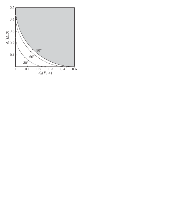
With the definition of distance in Eq.Β (6), the possible jointly measurable approximations to sharp observables 𝒫𝒫\mathcal{P}, 𝒬𝒬\mathcal{Q} are shown in Fig.Β 2. Taking the case of ΞΈ=90βˆ˜πœƒsuperscript90\theta=90^{\circ} first, the shaded area represents points where jointly measurable approximations π’œπ’œ\mathcal{A} and ℬℬ\mathcal{B} exist, with the distance from 𝒫𝒫\mathcal{P} and 𝒬𝒬\mathcal{Q} given on the xπ‘₯x and y𝑦y axis, respectively. The non-shaded area in the left down corner represents points where the requirement on the approximation is too high such that no jointly measurable approximations π’œπ’œ\mathcal{A} and ℬℬ\mathcal{B} exist. Moving from the left down corner to the right we relax our requirements on how closely π’œπ’œ\mathcal{A} approximates 𝒫𝒫\mathcal{P} until finaly we reach the boundary of the shaded region where some jointly measurable approximations exist. Similarly, moving up in the figure, we allow less strict approximation for 𝒬𝒬\mathcal{Q}. The boundary of the shaded area thus represents the optimal choice of jointly measurable approximations. Moving along the boundary curve one sees an expected trade off – if we require π’œπ’œ\mathcal{A} to better approximate 𝒫𝒫\mathcal{P}, we have to loosen our requirements on ℬℬ\mathcal{B} to preserve joint measurability. We also give boundary curves for the cases ΞΈ=60βˆ˜πœƒsuperscript60\theta=60^{\circ} and 30∘superscript3030^{\circ}. All these curves have been calculated numerically. Again, the region up right from these boundaries is the area where jointly measurable approximations exist. With decreasing ΞΈπœƒ\theta, the boundary moves towards the left down corner, which we could interpret as the two sharp observables 𝒫𝒫\mathcal{P} and 𝒬𝒬\mathcal{Q} becoming more easily jointly measurable. In the limit case ΞΈ=0βˆ˜πœƒsuperscript0\theta=0^{\circ}, the whole area would be shaded – we can find jointly measurable approximations with any desirable accuracy since the two sharp observables 𝒫𝒫\mathcal{P} and 𝒬𝒬\mathcal{Q} are then the same.

Refer to caption

Figure 2. Curves represent boundaries for jointly measurable approximations π’œπ’œ\mathcal{A} and ℬℬ\mathcal{B} of 𝒫𝒫\mathcal{P} and 𝒬𝒬\mathcal{Q} for different choices of angle ΞΈπœƒ\theta between the vectors 𝐩𝐩\mathbf{p} and πͺπͺ\mathbf{q}. The gray-shaded region represents the area where there exist jointly measurable pairs π’œπ’œ\mathcal{A} and ℬℬ\mathcal{B} for ΞΈ=90βˆ˜πœƒsuperscript90\theta=90^{\circ}.

The same problem has been studied analytically in Ref.Β [2] where the optimal solution was found in the case ds​(𝒫,π’œ)=ds​(𝒬,ℬ)subscriptπ‘‘π‘ π’«π’œsubscript𝑑𝑠𝒬ℬd_{s}(\mathcal{P},\mathcal{A})=d_{s}(\mathcal{Q},\mathcal{B}); the corresponding points in Fig.Β 2 are denoted by black dots. It was proved that the optimal π’œπ’œ\mathcal{A} and ℬℬ\mathcal{B} are then given by

(7) 𝐚=λ​𝐩+πͺ‖𝐩+πͺβ€–+(1βˆ’Ξ»)β€‹π©βˆ’πͺβ€–π©βˆ’πͺβ€–,𝐛=λ​𝐩+πͺ‖𝐩+πͺβ€–βˆ’(1βˆ’Ξ»)β€‹π©βˆ’πͺβ€–π©βˆ’πͺβ€–,formulae-sequenceπšπœ†π©πͺnorm𝐩πͺ1πœ†π©πͺnorm𝐩πͺπ›πœ†π©πͺnorm𝐩πͺ1πœ†π©πͺnorm𝐩πͺ\mathbf{a}=\lambda\frac{\mathbf{p}+\mathbf{q}}{\left\|\mathbf{p}+\mathbf{q}\right\|}+(1-\lambda)\frac{\mathbf{p}-\mathbf{q}}{\left\|\mathbf{p}-\mathbf{q}\right\|},\quad\mathbf{b}=\lambda\frac{\mathbf{p}+\mathbf{q}}{\left\|\mathbf{p}+\mathbf{q}\right\|}-(1-\lambda)\frac{\mathbf{p}-\mathbf{q}}{\left\|\mathbf{p}-\mathbf{q}\right\|}\,,

where Ξ»=12​(1+cos⁑θ2βˆ’sin⁑θ2)πœ†121πœƒ2πœƒ2\lambda=\tfrac{1}{2}(1+\cos\frac{\theta}{2}-\sin\frac{\theta}{2}). If ΞΈ=90βˆ˜πœƒsuperscript90\theta=90^{\circ}, then 𝐚=12β€‹π©πš12𝐩\mathbf{a}=\frac{1}{\sqrt{2}}\mathbf{p} and 𝐛=12​πͺ𝐛12πͺ\mathbf{b}=\frac{1}{\sqrt{2}}\mathbf{q}. Otherwise 𝐚𝐚\mathbf{a} and 𝐛𝐛\mathbf{b} are not parallel to 𝐩𝐩\mathbf{p} and πͺπͺ\mathbf{q} but they are somewhere between them as sketched in Fig.1.

4. Root-mean-square noise

In a series of recent articles [3, 4, 5] Ozawa has investigated noise and disturbance in quantum measurements. Assume that we try to measure an observable 𝒫𝒫\mathcal{P} (described by a selfadjoint operator σ𝐩subscript𝜎𝐩\sigma_{\mathbf{p}}) but we actually perform a measurement of π’œπ’œ\mathcal{A}. A precise measurement of 𝒫𝒫\mathcal{P} would mean that π’œ=π’«π’œπ’«\mathcal{A}=\mathcal{P}. Otherwise it is thought that we have a measurement of 𝒫𝒫\mathcal{P} with some noise. Ozawa defines the so-called root-mean-square noise Ο΅r​m​ssubscriptitalic-Ο΅π‘Ÿπ‘šπ‘ \epsilon_{rms} by the following formula [3]:

(8) Ο΅r​m​s​(𝒫,π’œ;ρ):=tr​[(π’œβ€‹[2]βˆ’π’œβ€‹[1]2+(Οƒπ©βˆ’π’œβ€‹[1])2)​ρ]12.assignsubscriptitalic-Ο΅π‘Ÿπ‘šπ‘ π’«π’œπœŒtrsuperscriptdelimited-[]π’œdelimited-[]2π’œsuperscriptdelimited-[]12superscriptsubscriptπœŽπ©π’œdelimited-[]12𝜌12\epsilon_{rms}(\mathcal{P},\mathcal{A};\rho):=\textrm{tr}\left[\left(\mathcal{A}[2]-\mathcal{A}[1]^{2}+(\sigma_{\mathbf{p}}-\mathcal{A}[1])^{2}\right)\rho\right]^{\tfrac{1}{2}}\,.

Here ρ𝜌\rho is an input state and π’œβ€‹[1]π’œdelimited-[]1\mathcal{A}[1] and π’œβ€‹[2]π’œdelimited-[]2\mathcal{A}[2] are the first and the second moment operators of π’œπ’œ\mathcal{A}, respectively.

Let now π’œπ’œ\mathcal{A} be a two outcome observable with outcomes Β±1plus-or-minus1\pm 1 and A𝐴A as in (2). A short calculation shows that if Ξ±=1𝛼1\alpha=1 then Ο΅r​m​s​(𝒫,π’œ;ρ)subscriptitalic-Ο΅π‘Ÿπ‘šπ‘ π’«π’œπœŒ\epsilon_{rms}(\mathcal{P},\mathcal{A};\rho) is a state independent number and we can define

(9) dr​m​s​(𝒫,π’œ):=Ο΅r​m​s​(𝒫,π’œ;ρ)=2​(1βˆ’πšβ‹…π©).assignsubscriptπ‘‘π‘Ÿπ‘šπ‘ π’«π’œsubscriptitalic-Ο΅π‘Ÿπ‘šπ‘ π’«π’œπœŒ21β‹…πšπ©d_{rms}(\mathcal{P},\mathcal{A}):=\epsilon_{rms}(\mathcal{P},\mathcal{A};\rho)=\sqrt{2(1-\mathbf{a}\cdot\mathbf{p})}\,.

Generally (i.e. Ξ±β‰ 1𝛼1\alpha\neq 1) we define dr​m​ssubscriptπ‘‘π‘Ÿπ‘šπ‘ d_{rms} to be the worst deviation over all input states. However, it can be shown that the optimal solutions are to be found among the operators having Ξ±=1𝛼1\alpha=1, so we again restrict our study to this case.

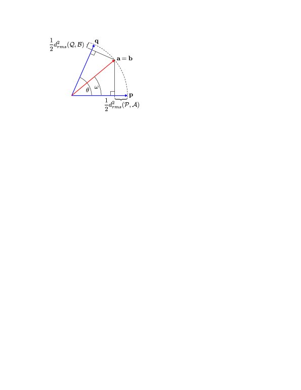
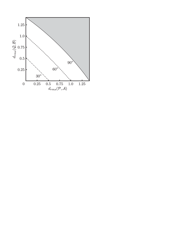
Assume that dr​m​s​(𝒫,π’œ)subscriptπ‘‘π‘Ÿπ‘šπ‘ π’«π’œd_{rms}(\mathcal{P},\mathcal{A}) is fixed and we are looking for the smallest possible number dr​m​s​(𝒬,ℬ)subscriptπ‘‘π‘Ÿπ‘šπ‘ π’¬β„¬d_{rms}(\mathcal{Q},\mathcal{B}) such that π’œπ’œ\mathcal{A} and ℬℬ\mathcal{B} are jointly measurable. According to Eq. (9), vectors 𝐚𝐚\mathbf{a} (𝐛𝐛\mathbf{b}) ending on the line perpendicular to 𝐩𝐩\mathbf{p} (πͺπͺ\mathbf{q}) have the same distance dr​m​s​(𝒫,π’œ)subscriptπ‘‘π‘Ÿπ‘šπ‘ π’«π’œd_{rms}(\mathcal{P},\mathcal{A}) (dr​m​s​(𝒬,ℬ)subscriptπ‘‘π‘Ÿπ‘šπ‘ π’¬β„¬d_{rms}(\mathcal{Q},\mathcal{B})). Going through all the possible pairs 𝐚𝐚\mathbf{a} and 𝐛𝐛\mathbf{b} satisfying the joint measurability condition (3), it can be shown that the optimal situation corresponds to the choice 𝐚=π›πšπ›\mathbf{a}=\mathbf{b}, where 𝐚𝐚\mathbf{a} is a unit vector and the angle Ο‰πœ”\omega between 𝐚𝐚\mathbf{a} and 𝐩𝐩\mathbf{p} is Ο‰=arccos⁑(1βˆ’12​dr​m​s​(𝒫,π’œ)2)πœ”112subscriptπ‘‘π‘Ÿπ‘šπ‘ superscriptπ’«π’œ2\omega=\arccos(1-\tfrac{1}{2}d_{rms}(\mathcal{P},\mathcal{A})^{2}); see Fig.Β 3. This solution means that in order to perform an optimal joint measurement, we measure spin in the direction 𝐚=π›πšπ›\mathbf{a}=\mathbf{b}. This is then regarded as an approximate version of both σ𝐩subscript𝜎𝐩\sigma_{\mathbf{p}} and Οƒπͺsubscript𝜎πͺ\sigma_{\mathbf{q}}. Combinations of dr​m​s​(𝒫,π’œ)subscriptπ‘‘π‘Ÿπ‘šπ‘ π’«π’œd_{rms}(\mathcal{P},\mathcal{A}) and dr​m​s​(𝒬,ℬ)subscriptπ‘‘π‘Ÿπ‘šπ‘ π’¬β„¬d_{rms}(\mathcal{Q},\mathcal{B}), for which jointly measurable approximations π’œπ’œ\mathcal{A} and ℬℬ\mathcal{B} exist, are shown in Fig.Β 4.

Refer to caption

Figure 3. For a fixed distance dr​m​s​(𝒫,π’œ)subscriptπ‘‘π‘Ÿπ‘šπ‘ π’«π’œd_{rms}(\mathcal{P},\mathcal{A}), the smallest distance dr​m​s​(𝒬,ℬ)subscriptπ‘‘π‘Ÿπ‘šπ‘ π’¬β„¬d_{rms}(\mathcal{Q},\mathcal{B}) is obtained when 𝐚=π›πšπ›\mathbf{a}=\mathbf{b} is the unit vector shown in the picture.

Refer to caption

Figure 4. Curves represent boundaries for jointly measurable approximations π’œπ’œ\mathcal{A} and ℬℬ\mathcal{B} of 𝒫𝒫\mathcal{P} and 𝒬𝒬\mathcal{Q} for different choices of angle ΞΈπœƒ\theta between the vectors 𝐩𝐩\mathbf{p} and πͺπͺ\mathbf{q}. The gray-shaded region represents the area where there exist jointly measurable pairs π’œπ’œ\mathcal{A} and ℬℬ\mathcal{B} for ΞΈ=90βˆ˜πœƒsuperscript90\theta=90^{\circ}.

The difference between the conclusions obtained here and in Section 3 can be explained by observing that while dssubscript𝑑𝑠d_{s} quantifies the accuracy of how π’œπ’œ\mathcal{A} approximates 𝒫𝒫\mathcal{P}, dr​m​ssubscriptπ‘‘π‘Ÿπ‘šπ‘ d_{rms} contains also a term which depends only on π’œπ’œ\mathcal{A}. Indeed,

(10) dr​m​s​(𝒫,π’œ)2=β€–π©βˆ’πšβ€–2+1βˆ’β€–πšβ€–2.subscriptπ‘‘π‘Ÿπ‘šπ‘ superscriptπ’«π’œ2superscriptnorm𝐩𝐚21superscriptnorm𝐚2d_{rms}(\mathcal{P},\mathcal{A})^{2}=\left\|\mathbf{p}-\mathbf{a}\right\|^{2}+1-\left\|\mathbf{a}\right\|^{2}\,.

The first part β€–π©βˆ’πšβ€–2superscriptnorm𝐩𝐚2\left\|\mathbf{p}-\mathbf{a}\right\|^{2} is related to the statistical distance dssubscript𝑑𝑠d_{s} while the second part 1βˆ’β€–πšβ€–21superscriptnorm𝐚21-\left\|\mathbf{a}\right\|^{2} can be interpreted as a quantification of the intrinsic unsharpness of π’œπ’œ\mathcal{A}.

Acknowledgements

This work was supported by projects CONQUEST, QAP and APVV.

References

  • [1] P.Β Busch. Unsharp reality and joint measurements for spin observables. Phys. Rev. D, 33:2253–2261, 1986.
  • [2] P.Β Busch and T.Β Heinonen. Approximate joint measurements of qubit observables. arXiv:0706.1415v1, 2007.
  • [3] M.Β Ozawa. Uncertainty relations for joint measurements of noncommuting observables. Phys. Lett. A, 320:367–374, 2004.
  • [4] M.Β Ozawa. Uncertainty relations for noise and disturbance in generalized quantum measurements. Ann. Physics, 311:350–416, 2004.
  • [5] M.Β Ozawa. Universal uncertainty principle in the measurement operator formalism. J. Opt. B Quantum Semiclass. Opt., 7(12):S672–S681, 2005.

Β