Determination of Dalitz plot slopes and asymmetries with the KLOE detector.
Abstract:
We have studied, with the KLOE detector at the DANE -Factory, the dynamics of the decay using mesons from the decay for an integrated luminosity = 450 . From a fit to the Dalitz plot density distribution we obtain a precise measurement of the slope parameters. An alternative parametrization relates the slopes to that for showing the consistency of KLOE results for both channels. We also obtain the best confirmation of the -invariance in the decay.
1 Introduction
The decay violates iso-spin invariance. Electromagnetic contributions to the process are very small [1] and the decay is induced dominantly by the strong interaction via the mass difference. The decay is therefore an ideal laboratory for testing chiral perturbation theory, ChPT. A three body decay222Both and are spinless, therefore there is no preferred direction. is fully described by two variables. We can choose two of the pion energies () in the rest frame, two of the three two pion masses squared () also called (). Note that is linear in and so on, cyclically. We use the Dalitz variables, which are linear combinations of the pion energies:
|
|
(1) |
where is the decay “-value”. The decay amplitude is given in [2] as:
| (2) |
where and is the average quark mass. MeV is the pion decay constant and must come from theory. From eq. 2 it follows that the decay rate for is proportional to . The transition is therefore very sensitive to if the amplitude M were known. At lowest order in ChPT:
| (3) |
From eq. 3, [2] one finds eV to be compared with the measured width of eV [3]. A one-loop calculation within conventional chiral perturbation theory (ChPT) [4], improves considerably the prediction:
| (4) |
but is still far from the experimental value. Higher order corrections [5] help but do not yet bring agreement with measurements of both total rate and Dalitz plot slopes. Good agreement is found combining ChPT with a non perturbative coupled channels approach using the Bethe Salpeter equation [6].
Therefore a precision study of the Dalitz plot, DP, is highly desirable. The amplitude squared is expanded around in power of and
| (5) |
The parameters ( ) can be obtained from a fit to the observed DP density and should be computed by the theory. Any odd power of in implies violation of charge conjugation.
2 The KLOE detector
Data were collected with the KLOE detector at DAΦNE [7], the Frascati collider, which operates at a center of mass energy MeV . The electron and positron beams collide with a crossing angle of mrad, resulting in a small momentum ( 13 MeV/c in the horizontal plane) of the produced mesons. The KLOE detector consists of a large cylindrical drift chamber (DC), surrounded by a fine sampling lead-scintillating fibers electromagnetic calorimeter (EMC) inserted in a 0.52 T magnetic field.
The DC [8], 4 m diameter and 3.3 m long, has full stereo geometry and operates with a gas mixture of 90% helium and 10% isobutane. Momentum resolution is . Position resolution in is 150 m and 2 mm. Charged tracks vertices are reconstructed with an accuracy of 3 mm.
The EMC [9] is divided into a barrel and two endcaps, for a total of 88 modules, and covers 98% of the solid angle. Arrival times of particles and space positions of the energy deposits are obtained from the signals collected at the two ends of the calorimeter modules, with a granularity of (4.4 x 4.4) cm2, for a total of 2240 cells arranged in five layers. Cells close in time and space are grouped into a calorimeter cluster. The cluster energy is the sum of the cell energies, while the cluster time and its position r are energy weighted averages. The respective resolutions are and .
The KLOE trigger [10] is based on the coincidence of at least two energy deposits in the EMC above a threshold that ranges between 50 and 150 MeV. In order to reduce the trigger rate due to cosmic rays crossing the detector, events with a large energy release in the outermost calorimeter planes are vetoed.
3 Signal selection and efficiency
This analysis refers to 450 pb-1 collected at DAΦNE in years 2001/02 corresponding to mesons produced.
At KLOE mesons are produced through the radiative decay . Accounting for the product of BR’s: we expect about four millions of events. A larger Monte Carlo (MC) sample corresponding to about times the amount of data has been used to study efficiencies and backgrounds.
Note that the recoil photon is almost monochromatic, with MeV, well separated from the softer photons from decay.
A photon is defined as an EMC cluster not associated to a DC track. We further require that , where is the arrival time at the EMC, is the distance of the cluster from interaction point, IP, is speed of light. The events selection is performed through the following steps:
-
1.
Events are first selected by a very loose offline filter to remove machine background (FILFO) and an event selection procedure (EVCL) assigning events into categories [11].
-
2.
We then require two opposite curvature tracks intersecting at a point (vertex) inside a cylinder with cm, cm centered at the IP. We require also three photons with and MeV. The angle between any photon pair must be to remove split showers.
-
3.
-
4.
A constrained kinematic fit is performed imposing 4-momentum conservation and for each photon. We retain events with a probability %, corresponding to . The fit significantly improves the photon energy resolution. The distribution is in reasonable agreement with MC prediction, as shown in fig.1; varying the cut on in the range [ 0.01, 0.15] has no significant effect on the analysis results, see section 5.
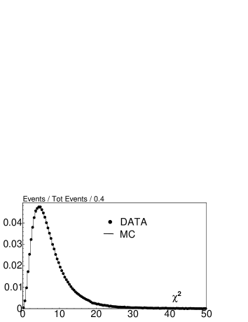
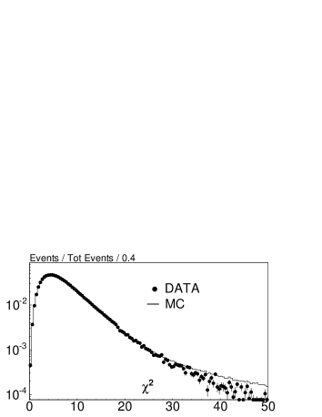
Figure 1: distribution for the kinematic fit. Left: linear scale. Right: log scale. -
5.
Finally we require:
-
(a)
320 MeV 400 MeV for the recoil photon, to reduce residual background from events.
-
(b)
550 MeV, to reduce residual background from events.
-
(c)
() for the two softest photons must satisfy 110160 MeV, to reduce residual background from decays with and from with ; and to eliminate the residual background from events with .
-
(a)
The selection efficiency is determined with the MC program [11] and checked with data control samples. In particular:
-
1.
The trigger efficiency evaluated by MC is %, with excellent data-MC agreement for the trigger sectors multiplicities.
-
2.
The effects of EVCL and FILFO are evaluated using a downscaled set of non filtered data with less stringent cuts in order to get a “minimum bias“ sample. On signal events the efficiency of the minimum bias selection is 99.88%. We have found that the EVCL procedure introduces a signal loss of 1.5%, as expected also from MC. The corresponding bias on the Dalitz plot parameters has been included in the systematic error. No bias is introduced by the FILFO procedure.
-
3.
The tracking and vertexing efficiencies have been estimated from the data-MC ratio observed in a sample of events with charged pion momenta in the same range as those from the decay [12]. These events can be selected with low background requiring the detection of the photons associated to the in the EMC and only one track in the DC and thus are suited to study on data the single charged track reconstruction efficiency, , and the charged vertex reconstruction efficiency, : This ratio is constant for all momenta, introducing no bias in the Dalitz plot distribution. All variables used in the fit are evaluated in the rest frame, which in the laboratory has a momentum of 363 MeV. Therefore to each momentum bin in the rest frame corresponds a wider interval in the lab; MC-data discrepancies are further diluted by this effect.
-
4.
A correction to the MC detection efficiency for low energy photons has been obtained by comparing the photon energy spectrum of a data subsample to the expected MC spectrum; the average correction factor is 0.964.
The overall selection efficiency, taking into account all the data-MC corrections is found to be %. The expected background contamination, obtained from MC simulation is 0.3%.
After background subtraction we remain with events.
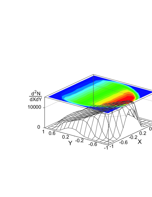
The Dalitz plot density is shown in fig.2.
The signal selection efficiency as function of the DP point is obtained by MC, for each bin, as the ratio:
| (6) |
where are respectively the reconstructed and generated DP populations. This approach accounts for resolution effects as long as the MC correctly reproduces the Dalitz plot shape; a first estimate of the Dalitz plot parameters to be used in the final MC was obtained from a preliminary fit to a data subsample. The efficiency has a smooth behavior all over the entire DP. The projections of are shown in fig.3.
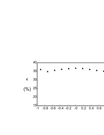
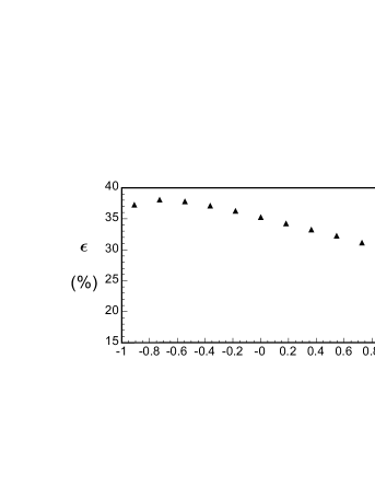
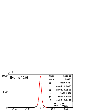
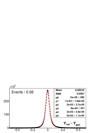
While the efficiency appears to be rather flat on (and symmetric as expected), it decreases approximately linearly with . In fact a large Y value means a low-momentum in the decay to which corresponds a lower tracking/vertexing efficiency. The resolutions from MC on the DP variables are shown in fig.4. The variable, which is proportional to the kinetic energy, is evaluated [13] as the average between the “direct” determination obtained from the energy and direction of the two clusters associated to the decay and the “indirect” determination : . Due to our excellent momentum resolution for charged tracks, the core of both distributions in fig.4 can be fitted with a gaussian with .
4 Fit of Dalitz plot
The expected Dalitz density is taken as:
| (7) |
with N being a normalization constant. The fit to the Dalitz plot is done in two dimensions, minimizing the function. Bins intersecting the Dalitz plot boundary are not included in the fit. The fit procedure has been tested on MC by verifying that the fit reproduces in output the same input values of the DP parameters.
The fit results for different forms of and for ==0.125 (154 bins fitted) are shown in Table 1. A fit with only quadratic terms gives a very low C.L. of or less. Including cubic terms as
| (8) |
results in much better fits with C.L. 70 %. In particular the coefficients of the term and of the term are clearly required while the other ones () turn out to be consistent with zero.
| dof | CL | ||||||
| 147 | 73% | 10905 | 1246 | 23 | 576 | 67 | 14010 |
| 149 | 74% | 10905 | 1246 | 576 | 14010 | ||
| 150 | 10695 | 1045 | 13010 | ||||
| 150 | 10413 | 1456 | 506 | ||||
| 151 | 10263 | 1256 |
As expected from -invariance and are consistent with zero. Ignoring them in the fit does not affect the other parameters.
Our final results for the Dalitz plot parameters are those shown in second
row of the table. The corresponding correlation coefficients are shown in eq.(16).
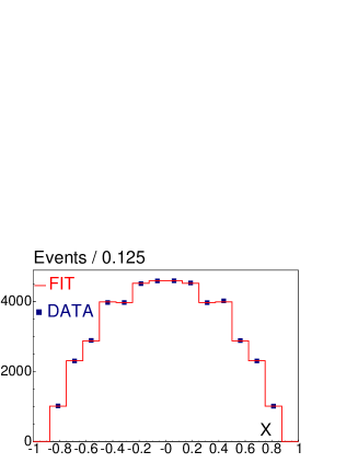
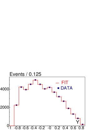
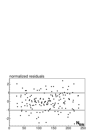
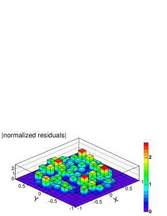
Fig 5 and Fig 6 show respectively a comparison
between fit and data for the projections in or and the normalized residuals as function of bin number (left) and DP variables (right).
5 Systematic uncertainties
We have estimated the systematics errors due to the following sources:
- Analysis cuts
-
We have moved separately the following cuts: in the range with a step of , in the range [0.01, 0.15] with a step of 0.05, in the range with a step of 5 MeV and in the range MeV with a step of 10 MeV. We find a negligible effect on the parameter estimates.
- Efficiency
-
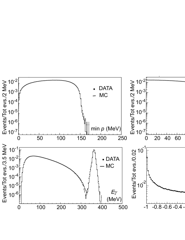
All reconstruction efficiencies have been checked with data, using control samples. We find excellent agreement between data and MC for various kinematical distributions (see fig.7). Concerning the photon detection efficiency we have checked that the error with which we estimate the ratio has a negligible impact on the estimate DP slope parameters. Only the EVCL procedure gives observable effects, as verified with the minimum bias sample.
- Resolution and binning
-
Energy resolution for the photons is checked by comparing Eγ distributions after the kinematic fit on data and MC. We find good agreement over the entire distributions. The drift chamber momentum resolution and absolute scale is checked run by run with the reconstructed mass from events. Binning size was changed up to a factor of two: .
- Background contamination
-
The main source of backgrounds are: with , and with . Changing the cut on in a wide range, corresponding to a background change from 0.7% to 0.2% , we find small changes for the parameter values.
- Stability with respect to data taking conditions
-
We have divided our data sample in 9 periods of about 50 each. We find that the results for each parameter are consistent with no change.
- Radiative corrections
-
We have generated decays, according to ref. [14]. The bin by bin ratio of the DP density for decays to that for decays can be fitted with a constant with /dof = corresponding to a CL of 46%.
The results are shown in Table 2.
| Source | ||||
|---|---|---|---|---|
| EVCL | 0.017 | 0.005 | 0.012 | 0.01 |
| binning | 0.008 +0.006 | 0.006 +0.006 | 0.007 +0.001 | 0.02 +0.02 |
| background | 0.001 +0.006 | 0.008 +0.006 | 0.007 +0.007 | 0.01 |
| Total | 0.019 +0.008 | 0.010 | 0.016 +0.007 | 0.02 |
For each effect mentioned above the systematic error has been estimated as the maximum parameter variation with respect to the reference value; the total systematic error is the sum in quadrature of the different contributions.
6 An alternative parametrization of the decay amplitude
We have also fitted the Dalitz plot with a different parametrization which takes into account the final state - rescattering. Since strong interactions are expected to mix the two isospin = 1 final states of the decay, it is possible to introduce a unique rescattering matrix which mixes the corresponding =1 decay amplitudes [15] , for which we have:
| (9) |
where:
| (10) |
According to ref. [15], the rescattering phases depend on the and variables333 We define and as: and with for and as
|
|
(11) |
where , , , are obtained from [16] after proper rescaling from kaon to mass. The complete amplitudes, keeping the expansion in powers of and up to quadratic terms, are then given by:
|
|
(12) |
and
| (13) |
We have fitted the Dalitz plot with the above parametrization and the fit results are given in Table 3.
| dof | 1000 | 1000 | 1000 | 1000 | |
|---|---|---|---|---|---|
| 150 | 71.120.07 | 13.710.04 | 0.460.03 | 0.760.02 |
7 Asymmetries
While the polynomial fit of the Dalitz plot density gives valuable information on the matrix element, integrated asymmetries are very sensitive in assessing the possible presence of violation in amplitudes of given . In particular left-right asymmetry - related to the parameter in our fit - tests violation with no specific constraint; quadrants asymmetry tests violation for and sextants asymmetry (for a definition see ref. [18]) tests violation for .
For this measurement care must be taken of possible slight differences between and reconstruction efficiencies. To this aim we estimate the MC efficiency separately for each region of the Dalitz plot, as the ratio between reconstructed and generated events in the region. This definition takes into account the resolution effects as well. From a sample of MC events we get:
| (quad.) | ||
| (sext.) |
We have checked these values estimating the asymmetries on Monte Carlo: these turn out to be all compatible with zero. We then evaluate the asymmetries on data by subtracting the MC expected background and correcting the “raw” asymmetries with the above efficiencies. We obtain:
Systematic uncertainties on the asymmetries are obtained from studying: a) sensitivity to background, by varying cuts, b) event selection (EVCL) by use of the minimum bias sample and c) MC-data comparison using events. In particular the tracking efficiency has been evaluated separately for the two charges, since in the MC a small but statistically significant difference in left and right efficiencies is evident. The above difference is due to a slightly different tracking efficiency vs for positive and negative pions because of nuclear interactions.
Since we require both tracks to be reconstructed the absolute value of the efficiency is not important for the asymmetry, but rather its dependence upon the pion momentum. The good data-MC agreement has been already demonstrated for both charges on the signal. We here use the control sample to check the agreement between data and MC for the and efficiencies as a function of momentum (see fig.8).
The control sample agrees well with MC within errors, and the data-MC ratio is well fitted by a constant.
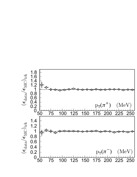
In order to assess the possible systematic uncertainties connected with the tracking efficiencies we adopt a conservative approach: we estimat the maximum positive or negative linear slopes compatible within one sigma with the fit of the distributions shown in fig.8. Then we have assumed that the two charges behave with opposite slopes. This gives us two possibilities: with positive slope and with negative slope or vice-versa. We have then reweighted the events according to these two possibilities and used the maximum difference observed in the asymmetries as the corresponding systematic error. The systematics connected with the asymmetries are shown in Table 4.
| Syst. Effect | Left-Right | Quadrant | Sextant |
|---|---|---|---|
| Background | |||
| EVCL | |||
| Efficiency | |||
| Total |
Therefore the final results for the asymmetries are:
|
|
where the first (second) is the statistical (systematic) error.
8 Conclusions
The results including the statistical uncertainties coming from the fit and the estimate of systematics are:
|
|
(15) |
Below we give the normalized correlation coefficients for the DP parameters.
| (16) |
The following comments are in order:
-
1.
the fitted value for the quadratic slope in is almost one half of the simple current algebra prediction (), thus calling for significant higher order corrections;
-
2.
the quadratic term in is unambiguously different from zero;
-
3.
similarly for the large cubic term in ;
-
4.
the fit results show correlations between the DP parameters. This should be properly taken into account for a correct error estimate when integrating the amplitude over phase space to get the decay width;
-
5.
fitting the Dalitz plot with an alternative parametrisation we obtained a prediction for the slope which is consistent with the PDG average and the KLOE measurement;
-
6.
we do not observe any evidence for violation in the decay since the and parameters of the Dalitz plot and the charge asymmetries are all perfectly consistent with zero.
Acknowledgements
We thank G. D’Ambrosio for many fruitful discussions. We thank the DAFNE team for their efforts in maintaining low background running conditions and their collaboration during all data-taking. We want to thank our technical staff: G.F. Fortugno and F. Sborzacchi for their dedicated work to ensure an efficient operation of the KLOE Computing Center; M. Anelli for his continuous support to the gas system and the safety of the detector; A. Balla, M. Gatta, G. Corradi and G. Papalino for the maintenance of the electronics; M. Santoni, G. Paoluzzi and R. Rosellini for the general support to the detector; C. Piscitelli for his help during major maintenance periods. This work was supported in part by EURODAPHNE, contract FMRX-CT98-0169; by the German Federal Ministry of Education and Research (BMBF) contract 06-KA-957; by the German Research Foundation (DFG), ’Emmy Noether Programme’, contracts DE839/1-4; by INTAS, contracts 96-624, 99-37; and by the EU Integrated Infrastructure Initiative HadronPhysics Project under contract number RII3-CT-2004-506078.
References
- [1] J.S. Bell and D.G. Sutherland, Current algebra and , Nucl. Phys. B 4 (1968) 315
- [2] For a review see J. Bijnens and J. Gasser, Eta Decays and Beyond in Chiral Perturbation Theory, Physica Scripta T99, (2002) 34.
- [3] Particle Data Group Collaboration, W. M. Yao et al., J. Phys. G 33 (2006) 1.
- [4] J. Gasser and H. Leutwyler, Chiral perturbation Theory to one loop, Annals Phys. 158 (1984) 142; Eta to 3 to one loop, Nucl. Phys. B 250 (1985) 539.
- [5] J. Bijnens and K. Ghorbani, at Two Loops in Chiral Perturbation Theory, J. High Energy Phys. 0711 (2007) 030.
- [6] B. Borasoy and R. Nissler, Hadronic and decays, Eur. Phys. J. A 26 (2005) 383.
- [7] DAFNE Collaboration, M. Zobov et al., DAFNE status and upgrade plans, arXiv: \arXivid0709.3696.
- [8] KLOE Collaboration, M. Adinolfi et al., The tracking detector of the KLOE experiment, Nucl. Instrum. Meth. A488 (2002) 51.
- [9] KLOE Collaboration, M. Adinolfi et al., The KLOE electromagnetic calorimeter, Nucl. Instrum. Meth. A 482 (2002) 364.
- [10] KLOE Collaboration, M. Adinolfi et al., The trigger system of the KLOE experiment, Nucl. Instrum. Meth. A 492 (2002) 134.
- [11] KLOE Collaboration, F. Ambrosino et al., Data handling, reconstruction, and simulation for the KLOE experiment, Nucl. Instrum. Meth. A 534 (2004) 403.
- [12] C. Di Donato, KLOE Note 214, $Φ→η' γ$ in $π^+ π^- 7 γ$ at KLOE.
- [13] F. Ambrosino, T. Capussela, F. Perfetto, KLOE Note 215, Dynamics of $$η→$π^+$$π^-$$π^0 $$$.
- [14] C. Gatti, Monte Carlo simulation for radiative kaon decays, Eur. Phys. J. C 45 (2005) 417.
- [15] G. D’Ambrosio, G. Isidori, CP violation in kaon decays, Int. J. Mod. Phys. A 13 (1998) 1.
- [16] G D’Ambrosio, G. Isidori, A. Pugliese and N. Paver, Strong rescattering in decays and low-energy meson interactions, Phys. Rev. D 50 (1994) 5767.
- [17] KLOE Collaboration, F. Ambrosino et al., Measurement of the slope parameter for the decay at KLOE, \arXivid0707.4137.
- [18] J. G. Layter et al., Measurement of the charge Asymmetry in the decay , Phys. Rev. Lett. 29 (1972) 316.