Cosmological Information in the Gravitational Lensing of Pregalactic HI

Abstract

We study the constraints which the next generation of radio telescopes could place on the nature of dark energy, dark matter and inflation by studying the gravitational lensing of high redshift 21 cm emission, and we compare with the constraints obtainable from wide-angle surveys of galaxy lensing. If the reionization epoch is effectively at $z\sim 8$ or later, very large amounts of cosmological information will be accessible to telescopes like SKA and LOFAR. We use simple characterizations of reionization history and of proposed telescope designs to investigate how well the two-dimensional convergence power spectrum, the three-dimensional matter power spectrum, the evolution of the linear growth function, and the standard cosmological parameters can be measured from radio data. The power spectra can be measured accurately over a wide range of wavenumbers at $z\sim 2$, and the evolution in the cosmic energy density can be probed from $z\sim 0.5$ to $z\sim 7$. This results in a characterization of the shape of the power spectra (i.e. of the nature of dark matter and of inflationary structure generation) which is potentially more precise than that obtained from galaxy lensing surveys. On the other hand, the dark energy parameters in their conventional parametrization ($\Omega_{\Lambda},w_{o},w_{a}$) are somewhat less well constrained by feasible 21 cm lensing surveys than by an all-sky galaxy lensing survey. This is because dark energy is felt primarily at relatively low redshifts in this model; 21 cm surveys would be more powerful than galaxy surveys for constraining models with “early” dark energy. Overall, the best constraints come from combining surveys of the two types. This results in extremely tight constraints on dark matter and inflation, and improves constraints on dark energy, as judged by the standard figure of merit, by more than an order of magnitude over either survey alone.

1 introduction

The now widely accepted cold dark matter (CDM) model combines with inflation-inspired scale-invariant primordial density fluctuations to provide a consistent explanation for cosmic microwave background (CMB) fluctuations, for type Ia supernova luminosity distances, for the clustering of galaxies in redshift surveys, for the galaxy cluster abundance and its evolution, and for the statistics both of weak gravitational lensing and of Ly$\alpha$ forest absorption in quasar spectra. This success comes at the cost of introducing several mysterious and apparently ad hoc constituents. Most of the matter is supposed to be dark, a weakly interacting neutral particle so far detected only through its gravitational effects. All structure is supposed to have originated during a very early period of accelerated expansion driven by an inflaton field which has been posited purely for this purpose. Finally the energy density of the Universe is apparently dominated today by a different and even more unexpected field, dark energy, which is similarly accelerating the present cosmic expansion. The nature of the dark energy and its relation to the rest of physics are unknown. Detailed measurements of the recent expansion history and of the corresponding gravitationally driven growth of structure provide the only known route to narrow down the possibilities. The techniques mentioned above can measure the expansion precisely out to $z\sim 4$ and the growth of structure out to $z\sim 1.5$. In this paper we investigate a new technique that complements, refines and greatly increases the precision of these methods by directly constraining both cosmic expansion and structural growth out to $z\sim 6$.

The spin temperature of neutral hydrogen during and before the epoch of reionization ($8\lower 2.15277pt\hbox{$\;\buildrel<\over{\sim}\;$}z\lower 2.15277pt\hbox{$\;\buildrel<\over{\sim}\;$}300$) fell out of thermal equilibrium with the CMB radiation, resulting in the absorption and emission of 21 cm radiation. There has been a great deal of interest in the prospect of detecting and mapping this radiation using low-frequency radio telescopes, Several suitable instruments are now under construction or in planning stages (see Furlanetto et al., 2006, for an extensive review). This radiation provides an excellent source for gravitational lensing studies. Structure is expected in the 21 cm emission down to arcsecond scales, and at each point on the sky there will be $\sim 1000$ statistically independent regions, separated in redshift (and thus frequency) that can in principle be observed. Gravitational lensing coherently distorts the 21 cm brightness temperature maps at different frequencies. This coherent distortion can be distinguished from intrinsic structure in the HI gas if enough independent redshifts are observed. In this way a map of the foreground density can be constructed (Zahn & Zaldarriaga, 2006; Metcalf & White, 2007; Hilbert et al., 2007; Lu & Pen, 2007).

Observing the 21 cm radiation at high redshift will be challenging. It will require large arrays of radio telescopes working at low frequencies ( $\sim 100$ to 200 MHz). At these frequencies foregrounds – terrestrial, galactic and extragalactic – are very large and will need to be subtracted by complex and as yet untested procedures (Furlanetto et al., 2006). This challenge is currently being addressed by several observational teams (see section 6).

In addition to the noise associated with mapping the brightness temperature, the lensing signal has an additional intrinsic noise component which comes from the unknown intrinsic structure of the 21 cm brightness temperature distribution. This noise cannot be reduced by increasing the collecting area of the telescope, by increasing the integration time or by improving the removal of foregrounds. Metcalf & White (2007) showed that if the signal-to-noise in the brightness temperature map at each frequency is greater than one, then the noise in the mass map will be close to the intrinsic value. Increasing the frequency resolution of the radio observations increases the number of effectively independent regions along the line-of-sight until the bandwidth becomes smaller than the correlation length in the redshift direction of the brightness temperature distribution. If the bandwidth is matched to the correlation length, the intrinsic noise is minimized. The correlation length in turn depends on beam size, and is smaller for smaller beams. Thus unlike galaxy lensing surveys, the intrinsic noise for 21 cm lensing decreases with increasing telescope resolution. In practice, there is a trade-off because smaller bandwidth means less flux, but this can be compensated by increasing collecting area and/or integration time. The noise is also affected by the range of frequency (i.e. redshift) over which the 21 cm radiation can be detected. The low-frequency limit is set by the telescope and/or the ability to subtract foregrounds. The high-frequency limit is typically set by the reionization of the universe, after which the amount of intergalactic HI is small.

In Hilbert et al. (2007) we simulated how well an idealized optimal telescope would be able to map the 2 dimensional distribution of matter. In this paper, we study how well radio telescopes with specifications similar to those of instruments currently being built or planned will be able to constrain cosmological parameters, in particular those related to the nature of dark matter, dark energy and inflation.

This paper is organized as follows. The next two sections introduce the formalism we use to study lensing in general and lensing of the 21 cm radiation in particular. In section 4 we develop a formalism for extracting cosmological information and density maps from such lensing data. In section 5 we discuss the relevant aspects of reionization and the simple reionization model we use to make quantitative predictions. The telescope parameters used in our predictions are given in section 6. Section 7 contains predictions for the noise levels in various quantities. A summary of our results and of future prospects is given in the last section.

2 lensing preliminaries

Gravitational lensing shifts the observed position of each point in the image of a distant source. Take the observed angular position on the sky to be $\vec{\theta}$ and the position in the absence of lensing to be $\vec{\beta}$. The first-order distortion in the image is expressed by the derivatives of the mapping between these angles. The distortion matrix is commonly decomposed into the convergence $\kappa$ and two components of shear, $\bf\gamma$, defined by

$$\left[\frac{\partial\beta}{\partial\theta}\right]=\left(\begin{array}[]{ccc}1-\kappa+\gamma_{1}&\gamma_{2}\\ \gamma_{2}&1-\kappa-\gamma_{1}\end{array}\right).$$ (1)

To lowest order and to an excellent approximation (Vale & White, 2003) the convergence is related directly to the distribution of matter through

$$\kappa\left(\vec{\theta},z_{s}\right) =\frac{3}{4}H_{o}\Omega_{m}\int_{0}^{\infty}dz~{}\frac{(1+z)}{E(z)}g\left(z,z_{s}\right)\delta\left(\vec{\theta},z\right)$$ (2)

$$\simeq\frac{3}{4}H_{o}\Omega_{m}\sum_{i}\delta\left(\vec{\theta},z_{i}\right)\int_{z_{i}-\delta z}^{z_{i}+\delta z}dz~{}\frac{(1+z)}{E(z)}g\left(z,z_{s}\right)$$

$$=\sum_{i}G(z_{i},z_{s})\delta\left(\vec{\theta},z_{i}\right)$$ (3)

with

$$g(z,z_{s})=\int_{z}^{\infty}dz^{\prime}~{}\eta\left(z^{\prime},z_{s}\right)\frac{D(z,0)D(z^{\prime},z)}{D(z^{\prime},0)}.$$ (4)

The weighting function for the source distance distribution, $\eta(z)$, is normalized to unity. $D(z^{\prime},z)$ is the angular size distance between the two redshifts and $\delta(\vec{x},z)$ is the fractional density fluctuation at redshift $z$ and perpendicular position $\vec{x}$. The function

$$E(z)=\sqrt{\Omega_{m}(1+z)^{3}+\Omega_{\Lambda}(1+z)^{3f(z)}+(1-\Omega_{m}-\Omega_{\Lambda})(1+z)^{2}},$$ (5)

where $\Omega_{m}$ and $\Omega_{\Lambda}$, are the present day densities of matter and dark energy measured in units of the critical density. The function describing the evolution of dark energy with redshift can be written

$$f(z)=\frac{-1}{\ln(1+z)}\int^{0}_{-\ln(1+z)}\left[1+w(a)\right]~{}d\ln a$$ (6)

where $w(a)$ is the equation of state parameter for the dark energy – the ratio of the of its pressure to its density – and $a=(1+z)^{-1}$ is the scale parameter. Where not otherwise mentioned, we will assume the universe is flat, $\Omega_{m}+\Omega_{\Lambda}=1$, and $w(a)=-1$.

Equation (2) shows that $\kappa$ can be interpreted as a kind of projected dimensionless surface density. For our purposes it is convenient to express equation (3) as a matrix equation,

$${\it\bf K}={\rm\bf G}\boldsymbol{\delta},$$ (7)

where the the components of ${\bf K}$ are the convergences running over all position angles $\vec{\theta}$ and source redshifts, $z_{s}$. The components of the vector $\boldsymbol{\delta}$ run over all position angles and foreground redshifts $z_{i}$. The matrix ${\rm\bf G}$ is a function of most of the global cosmological parameters – $\Omega_{m}$, $\Omega_{\Lambda}$, $w$, etc – and is independent of position on the sky. The latter property makes these equations equally valid when $\kappa$ and $\delta$ are transformed from angular space to spherical harmonic space or to the $u$-$v$ plane where interferometer observations are carried out.

When considering 21 cm lensing we will make the approximation $\eta(z,z_{s})=\delta^{D}(z-z_{s})$, a Dirac delta function, for each band observed corresponding to a frequency of $\nu=1420(1+z_{s})^{-1}$ MHz. This is reasonable because angular size distances vary little within a single band, but it is not true in the case of galaxy lensing which we address in section 7.4.

3 lensing of pregalactic HI

Many convergence estimators are possible and can be expressed either in real-space (which is more easily visualised) or in Fourier-space (which is more easily related to interferometer observations in visibility-space). Metcalf & White (2007) gave a real-space estimator for $\kappa$ that has some advantages, but to simplify the present exposition we here use a Fourier-space estimator based on that introduced by Hu & Okamoto (2002) for the case of CMB lensing, and extended by Zahn & Zaldarriaga (2006) (and in the appendix of Metcalf & White (2007)) to allow estimation of the 2-dimensional $\kappa$ field from 3-dimensional 21 cm data. Our treatment here parallels this earlier work, although with some significant differences in the source redshift weighting.

In the appendix of Metcalf & White (2007)) we applied the Hu & Okamoto (2002) estimator for the Fourier transform of the convergence, $\kappa(\boldsymbol{\ell},\nu)$, to each frequency band and then combined them optimally to find a final estimate for $\kappa(\boldsymbol{\ell})$. This has the disadvantage of requiring that an optimal bandwidth be found numerically which will be a function of both $|\boldsymbol{\ell}|$ and frequency. An alternative method for combining frequencies is developed in Zahn & Zaldarriaga (2006). They use the Fourier transform of $T(\ell,\nu)$ in the frequency direction as well as the angular directions and then find a convergence estimator of the form

$$\hat{\kappa}\left(\boldsymbol{\ell}\right)=\int d^{2}\boldsymbol{\ell}^{\prime}\sum_{k_{1}}\sum_{k_{2}}~{}\chi(\boldsymbol{\ell}^{\prime},\boldsymbol{\ell},k_{1},k_{2})T^{*}(\boldsymbol{\ell}^{\prime},k_{1})T^{*}(\boldsymbol{\ell}^{\prime}-\boldsymbol{\ell},k_{2})$$ (8)

where $\boldsymbol{\ell}$ is the Fourier dual of the angle and $k$ is the discrete Fourier mode in the radial direction. The kernel $\chi(\boldsymbol{\ell}^{\prime},\boldsymbol{\ell},k_{1},k_{2})$ is found by minimizing the noise while constraining the average to be the convergence. This has the apparent advantage that the bandwidth does not come into the calculation, but, in practice, an equally arbitrary frequency scale will need to be imposed. In deriving the noise in their estimator Zahn & Zaldarriaga (2006) make the implicit assumption that the temperature field is statistically homogeneous in frequency. This assumption results in the Fourier modes being uncorrelated which greatly simplifies the calculation. In practice the temperature field will be inhomogeneous because the noise will be a strong function of frequency and because of the evolution of structure and ionization. As a result their estimator will not be optimal for a finite range in frequency only for $\Delta\nu/\nu\ll 1$. This problem was avoided in our method.

In this paper we will adopt a hybrid method for estimating the convergence that avoids many of the shortcomings the previous two methods. We use the Zahn & Zaldarriaga (2006) estimator within frequency bands which are larger than our previous bandwidths and the minimum band width of the telescope, but small enough that no significant inhomogeneity in the noise and brightness temperature structure is expected. This avoids having to find the optimal bandwidth. We then linearly combine these $\kappa(\boldsymbol{\ell},\nu)$ estimates in optimal ways as described in detail in section 4. We show that the correlations between convergence estimates at different frequencies is not significant if the bands widths are taken to be $\sim 1$ MHz.

The optimal kernel for estimator (8) under the assumption of homogeneity and Gaussianity within the band is

$$\chi(\boldsymbol{\ell}^{\prime},\boldsymbol{\ell},k_{1},k_{2},\nu)=\omega(\boldsymbol{\ell},\nu)|\boldsymbol{\ell}|^{2}\delta_{k_{1}k_{2}}~{}~{}~{}~{}~{}~{}~{}~{}~{}~{}~{}~{}~{}~{}~{}~{}~{}~{}~{}~{}~{}~{}~{}~{}~{}~{}~{}~{}~{}~{}~{}$$

$$~{}~{}~{}~{}~{}~{}~{}~{}\times\frac{\left[\boldsymbol{\ell}\cdot\boldsymbol{\ell}^{\prime}\,C_{\nu}(\ell^{\prime},k_{1})+\boldsymbol{\ell}\cdot(\boldsymbol{\ell}-\boldsymbol{\ell}^{\prime})\,C_{\nu}(|\boldsymbol{\ell}^{\prime}-\boldsymbol{\ell}|,k_{1})\right]}{C^{T}_{\nu}(\ell^{\prime},k_{1})C^{T}_{\nu}(|\boldsymbol{\ell}^{\prime}-\boldsymbol{\ell}|,k_{1})}$$ (9)

where $C^{T}_{\nu}(\ell,k)$ is the power spectrum of the actual temperature, while $C_{\nu}(\ell,k)=C^{T}_{\nu}(\ell,k)+C^{N}_{\nu}(\ell,k)$ is the observed power spectrum which includes noise. The normalization is

$$\omega(\boldsymbol{\ell},\nu)=~{}~{}~{}~{}~{}~{}~{}~{}~{}~{}~{}~{}~{}~{}~{}~{}~{}~{}~{}~{}~{}~{}~{}~{}~{}~{}~{}~{}~{}~{}~{}~{}~{}~{}~{}~{}~{}~{}~{}~{}~{}~{}~{}~{}~{}~{}~{}~{}~{}~{}~{}~{}~{}~{}~{}~{}~{}$$

$$\frac{1}{2}\left[\sum_{k}\int d^{2}{\ell}^{\prime}\frac{\left[\boldsymbol{\ell}\cdot\boldsymbol{\ell}^{\prime}\,C_{\nu}(\ell^{\prime},k)+\boldsymbol{\ell}\cdot(\boldsymbol{\ell}-\boldsymbol{\ell}^{\prime})\,C_{\nu}(|\boldsymbol{\ell}^{\prime}-\boldsymbol{\ell}|,k)\right]^{2}}{C^{T}_{\nu}(\ell^{\prime},k)C^{T}_{\nu}(|\boldsymbol{\ell}^{\prime}-\boldsymbol{\ell}|,k)}\right]^{-1}.$$ (10)

In the limit of an infinitely large beam the correlation between modes is

$$\left\langle\hat{\kappa}\left({\bf L},k_{1}\right)\hat{\kappa}^{*}\left({\bf L}^{\prime},k_{2}\right)\right\rangle=2(2\pi)^{4}\delta^{D}\left({\bf L}-{\bf L}^{\prime}\right)\delta_{k_{1}k_{2}}~{}~{}~{}~{}~{}~{}~{}~{}~{}~{}~{}$$

$$\times\int d^{2}{\ell}^{\prime}~{}\chi\left(\boldsymbol{\ell}^{\prime},{\bf L},k_{1}\right)^{2}C^{T}_{\nu}(\ell^{\prime},k_{1})C^{T}_{\nu}(|\boldsymbol{\ell}^{\prime}-{\bf L}|,k_{1})$$ (11)

$$=(2\pi)^{2}\delta^{D}\left({\bf L}-{\bf L}^{\prime}\right)\delta_{k_{1}k_{2}}N^{\hat{\kappa}}(L,\nu)$$ (12)

To simplify analysis, it has here been assumed that the temperature (i.e. the 21 cm emissivity) is Gaussian distributed so that the fourth moment can be written as products of second moments. The actual temperature distribution will be non-Gaussian because of non-uniform spin temperature, peculiar velocities, nonlinear structure formation, and non-uniform ionization. The importance of nonlinear structure formation in this context has been highlighted by Lu & Pen (2007). Some of these non-Gaussian effects, such as non-uniform ionization, cannot be usefully quantified at this time. The Gaussian approximation should be valid at least before significant reionization occurs and is probably good while the reionized regions are significantly smaller than the resolution of the telescope.

The finite telescope beam will cause correlations in the noise, $\langle\kappa(\boldsymbol{\ell})\kappa^{*}(\boldsymbol{\ell}+\delta\boldsymbol{\ell})\rangle\neq 0$, when $\delta\ell\lower 2.15277pt\hbox{$\;\buildrel<\over{\sim}\;$}2\pi\sigma_{u}$ where $\sigma_{u}$ is the width of the beam in $u$-$v$ space (Metcalf & White, 2007). These correlations can be taken into account, but for simplicity they will not be considered here.

The noise in $\hat{\kappa}(\ell,\nu)$ within one frequency band is

$$N^{\hat{\kappa}}(\ell,\nu)=\frac{(2\pi)^{2}}{2}~{}~{}~{}~{}~{}~{}~{}~{}~{}~{}~{}~{}~{}~{}~{}~{}~{}~{}~{}~{}~{}~{}~{}~{}~{}~{}~{}~{}~{}~{}~{}~{}~{}~{}~{}~{}~{}~{}~{}~{}~{}~{}~{}~{}~{}~{}~{}~{}~{}~{}~{}~{}~{}~{}~{}$$

$$\times\left[\sum_{k}\int d^{2}\ell^{\prime}~{}\frac{\left[\boldsymbol{\ell}\cdot\boldsymbol{\ell}^{\prime}\,C_{\nu}(\ell^{\prime},k)+\boldsymbol{\ell}\cdot(\boldsymbol{\ell}-\boldsymbol{\ell}^{\prime})\,C_{\nu}(|\boldsymbol{\ell}^{\prime}-\boldsymbol{\ell}|,k)\right]^{2}}{C^{T}_{\nu}(\ell^{\prime},k)C^{T}_{\nu}(|\boldsymbol{\ell}^{\prime}-\boldsymbol{\ell}|,k)}\right]^{-1}$$ (13)

Because the estimator (8) is a sum over all the observed pairs of visibilities, it will (by the central limit theorem) be close to Gaussian distributed even though it is quadratic in the visibilities. In the remainder of this paper this property will be assumed. The intrinsic noise limit corresponds to the case where $C_{\nu}(\ell)=C^{T}_{\nu}(\ell)$.

In real data the temperature distribution will not be Gaussian, the foregrounds will not be perfectly subtracted and will produce spurious frequency correlations, there will be holes in the area surveyed around bright point sources, there will be a finite and irregular beam, and the coverage of the $u$-$v$ plane will not be complete. It is also true that the convergence estimator was derived in the weak lensing limit ($\kappa\ll 1$) which will not be valid in all regions of the sky. All these complications make it unclear at the present time what estimator will be optimal for a real experiment. We nevertheless believe that the above relatively simple assumptions should give a good indication of what can be expected.

4 parameter estimation and density mapping

The noise in $\hat{\kappa}(\ell,z)$ for different bands and different $\ell$ will, to a good approximation, be statistically independent. The data vector will be defined as

$${\bf D} =\hat{\bf K}-{\bf K}$$ (14)

$$=\hat{\bf K}-{\bf G}\boldsymbol{\delta}$$ (15)

where the components run over all the combinations of $z_{i}$ and $\ell$ that are measured.

In this case the log of the likelihood function can be written

$$\ln{\mathcal{L}}=-\frac{1}{2}{\bf D}^{\dagger}{\rm\bf N}^{-1}{\bf D}-\frac{1}{2}|{\rm\bf N}|-H.$$ (16)

An additional function $H$ has been added to represent a prior distribution on the parameters or, in the context of density reconstruction, a regularization. As written so far the free parameters include all the cosmological parameters and all the foreground densities in each redshift bin. The noise covariance matrix is approximately

$${\rm\bf N}_{ij} =I_{ij}N^{\hat{\kappa}}(\ell_{i},\nu_{i})$$ (17)

$$\simeq\delta_{ij}I(\ell_{i},\nu_{i})N^{\hat{\kappa}}(\ell_{i},\nu_{i}).$$ (18)

The matrix $I_{\nu\nu^{\prime}}({\bf L})$ has been introduced to express possible cross-correlations between frequency bands. It will be normalized so that $I_{\nu\nu}({\bf L})=1$. The second line further simplifies this by assuming that the noise is equal in frequency bands that have significant correlation between them. In is case the $I_{\nu\nu^{\prime}}({\bf L})$ matrix can be made into a factor, $I(\ell,\nu)=\sum_{\nu^{\prime}}I_{\nu\nu^{\prime}}(\ell)$. In our studies here $I_{\nu\nu^{\prime}}({\bf L})\simeq\delta_{\nu\nu^{\prime}}$ or $I(\ell,\nu)\simeq 1$ since the correlations between the wide bands used ($\sim 1$ MHz) are small, but it is possible that foreground subtraction in particular might introduce significant correlations between frequency bins. Foreground subtraction will not be discussed in detail here, but we will retain the off-diagonal elements in our formalism. There will also be some off-diagonal elements to ${\bf N}_{ij}$ between different $\ell$ values caused by the finite beam of the telescope. Thses could be incorporated in a future analysis.

The maximum likelihood estimate for any parameter can be found by maximizing (16) with respect to that parameter. The error in this estimator is often forecasted using the Fisher matrix defined as

$${\rm\bf F}_{ij}=-\left\langle\frac{\partial^{2}\ln\mathcal{L}}{\partial p_{i}\partial p_{j}}\right\rangle.$$ (19)

The expected error in the parameter $p_{a}$, marginalized over all other parameters, is $\sigma_{a}^{2}\simeq\left({\rm\bf F}^{-1}\right)_{aa}$. The unmarginalized error estimate (the error when all other parameters are held fixed) is $\left({\rm\bf F}_{aa}\right)^{-1}$.

Often the parameters of physical interest have highly correlated noise, quantified by the off-diagonal elements in ${\bf F}$. As a result $\sigma_{a}$ can be a deceptive measure of how well the data constrains the parameter set as a whole. A way to mitigate this is to find the transformation that diagonalizes ${\bf F}$

$${\rm\bf F}={\bf V}^{\dagger}\boldsymbol{\lambda}{\bf V}.$$ (20)

This defines linear combinations of the parameters ${\bf\hat{p}}={\bf V}{\bf p}$ that are uncorrelated and have variances $\lambda_{aa}^{-1}$. This will be used in section 7.3.

4.1 Tomography

If one is primarily interested in reconstructing the cosmic mass density distribution, the background cosmology can be held fixed and $\mathcal{L}$ can be maximized with respect to the pixelized foreground density. This can be done in 2-D by approximating $\kappa$ as independent of $\nu$, in which case the solution that maximizes (16) is

$$\kappa(\vec{\ell})=\frac{\sum_{\nu\nu^{\prime}}{\bf N}_{\nu\nu^{\prime}}^{-1}(\ell)~{}\hat{\kappa}(\vec{\ell},\nu)}{\sum_{\nu\nu^{\prime}}{\bf N}_{\nu\nu^{\prime}}^{-1}(\ell)},$$ (21)

with corresponding noise,

$$N(\ell) =\frac{1}{\sum_{\nu\nu^{\prime}}{\bf N}_{\nu\nu^{\prime}}^{-1}(\ell)}$$ (22)

$$\simeq\frac{1}{\sum_{\nu}\left[I(\ell,\nu)N(\ell,\nu)\right]^{-1}},$$ (23)

which is uncorrelated between $\vec{\ell}$ values that are separated by more than the resolution of the telescope. Here no regularizing function is used ($H=0$). This is the result derived by Metcalf & White (2007).

A 3-D density reconstruction can be obtained by maximizing (16) with respect to the components of $\boldsymbol{\delta}$. For $H=0$, the solution, after some algebra and taking into account that ${\bf N}$ is symmetric, is

$$\boldsymbol{\delta}=\left[{\bf G}^{\dagger}{\bf N}^{-1}{\bf G}\right]^{-1}{\bf G}^{\dagger}{\bf N}^{-1}\hat{\bf K}.$$ (24)

Essentially the same result was obtained by Hu & Keeton (2002) for density reconstruction using galaxy lensing data in real-space. This requires that the matrix in braces be invertible. In the special case where ${\bf G}$ is invertible the estimator is simply $\boldsymbol{\delta}={\bf G}^{-1}\hat{\bf K}$. The noise covariance matrix for the reconstruction (24) is

$${\bf N}_{\delta}=\left[{\bf G}^{\dagger}{\bf N}^{-1}{\bf G}\right]^{-1}.$$ (25)

This noise will be highly correlated between $\delta$’s.

The regularization function in (16) can be used to improve the density reconstruction at the expense of making some assumptions about the statistical properties of the underlying density distribution. One choice is to assume that this distribution is Gaussian, in which case

$$H =\frac{1}{2}\boldsymbol{\delta}^{\dagger}{\bf C}^{-1}_{\delta}\boldsymbol{\delta}$$ (26)

$$=\frac{1}{2}\sum_{i\ell}\frac{\delta(z_{i},\vec{\ell})^{2}}{C_{\delta}(z_{i},\ell)},$$ (27)

where $C_{\delta}(z,\ell)$ is the angular power spectrum of mass within the redshift bin labeled by $z_{i}$. This is equivalent to a Wiener filter. The optimal estimator (24) and the noise (25) will be modified in this case, but can be derived in the same way. In addition to smoothing the noisy map, regularization provides a well behaved way to deal with missing telescope baselines and with holes in coverage due to foreground sources. Other regularization schemes could include an entropic prior or filters designed to emphasize localized mass lumps (Hu & Keeton, 2002).

4.2 Cosmological parameter estimation

Estimates of cosmological parameters and statistical information about the underlying mass density distribution can be extracted from 21 cm data without constructing density maps. The actual distribution of matter can be marginalized over assuming a suitable prior. This procedure can give surprisingly precise results, even when noise levels are far too high for a meaningful density reconstruction to be possible.

According to the standard model of structure formation, the components of ${\bf K}$ (i.e. $\kappa(\boldsymbol{\ell},\nu)$) will be normally distributed for $\ell$ less than several thousand (Takada & Jain, 2004). In this case a prior $H=\frac{1}{2}{\bf K}^{\dagger}{\bf C}_{\kappa}^{-1}{\bf K}$ can be used and the likelihood function can be integrated over all components of ${\bf K}$ – i.e. over all possible convergence maps. ${\bf C}_{\kappa}$ here is the (cross-)power spectrum of the convergence for two different source redshifts,

$$\left[{\bf C}_{\kappa}\right]_{ij}=\left\langle\kappa(\vec{\ell},z_{i})\kappa(\vec{\ell},z_{j})\right\rangle.$$ (28)

This can be calculated using expression (2) and a model for the matter power spectrum. The resulting likelihood function has the same form as (16)

$$\ln{\mathcal{L}}=-\frac{1}{2}\hat{\bf K}^{\dagger}{\rm\bf C}^{-1}\hat{\bf K}-\frac{1}{2}|{\rm\bf C}|,$$ (29)

where the noise matrix, ${\bf N}$, is now replaced with the covariance matrix,

$${\bf C}={\bf N}+{\bf C}_{\kappa}.$$ (30)

Since $\ell$-modes separated by more than the resolution of the telescope will not be correlated, we can break the likelihood function up into factors representing each resolved region in $\ell$-space (Metcalf & White, 2007). The result is that there are $\sim(2\ell+1)f_{\rm sky}$ independent measured modes for each value of $\ell$, where $f_{\rm sky}$ is the fraction of sky surveyed. The Fisher matrix can then be further simplified to the widely used form,

$${\bf F}_{ab}=\frac{1}{2}\sum^{\ell_{\rm max}}_{\ell=\ell_{\rm min}}(2\ell+1)f_{\rm sky}{\rm tr}\left[{\bf C}^{-1}{\bf C},_{a}{\bf C}^{-1}{\bf C},_{b}\right]~{}.$$ (31)

A quantity of particular interest that will be calculated later in this paper is the noise variance in the 2-D convergence power spectrum estimate. This is easily derived from (31) as

$$\Delta C_{\kappa}(\ell)=\sqrt{\frac{2}{(2\ell+1)f_{\rm sky}}}\,\left[C_{\kappa}(\ell)+N(\ell)\right],$$ (32)

where $N(\ell)$ is given by (22). The first term represents the sample or cosmic variance, and the second the noise in the $\kappa$ estimate itself. To increase the signal-to-noise the average power (known as the band-power) can be estimated within a bin of width $\Delta\ell$ larger than the resolution limit of the survey, $\delta\ell\sim f_{\rm sky}^{-1/2}$. The noise in the band-power is the above divided by the square root of the number of independent measurements within the band,

$$\Delta C_{\kappa}\left(\ell,\Delta\ell\right)\simeq\frac{\Delta C_{\kappa}(\ell)}{f_{\rm sky}^{1/4}\Delta\ell^{1/2}}.$$ (33)

5 reionization model

The fluctuations in the brightness temperature depend on the spin temperature, $T_{s}$, the ionization fraction, $x_{\rm H}$ and the density of HI through

$$\delta T_{b}\simeq 24(1+\delta_{b})x_{\rm H}\left(\frac{T_{s}-T_{\rm CMB}}{T_{s}}\right)\left(\frac{\Omega_{b}h^{2}}{0.02}\right)$$

$$\times\left(\frac{0.15}{\Omega_{m}h^{2}}\frac{1+z}{10}\right)^{1/2}\mbox{ mK}$$ (34)

(Field, 1959; Madau et al., 1997). As is commonly done, we will assume that the spin temperature is much greater than the CMB temperature. This leaves fluctuations in $x_{H}$, and the baryon density $\delta_{b}=(\rho_{b}-\overline{\rho}_{b})/\overline{\rho}_{b}$ as the sources of brightness fluctuations. We will make the simplifying assumption that $x_{\rm H}=1$ until the universe is very rapidly and uniformly reionized at a redshift of $z_{\rm reion}$. Realistically, the reionization process will be inhomogeneous and may extend over a significant redshift range. This will increase $C_{\nu}(\ell)$ by perhaps a factor of 10 on scales larger the characteristic size of the ionized bubbles (Zaldarriaga et al., 2004) and thus might be expected to reduce the noise in the lensing map, $\hat{\kappa}(\vec{\theta})$, significantly. However, the noise, (3), has been derived assuming that the fourth order statistics of $\delta T_{b}$ can be approximated by the values appropriate for a Gaussian random field. If this approximation holds, the lensing noise will indeed be reduced during reionization, but this is uncertain, since the temperature distribution will clearly not be Gaussian at this time, especially when the neutral fraction is low. Incorporating a more realistic ionization history is difficult and requires further work. A definitive resolution of these uncertainties will not, in any case, be possible until the observations are taken.

With real data one will not need to rely on an assumption of Gaussianity. It will be possible to derive the uncertainties by bootstrap techniques, since the higher order statistics of the temperature variations can be estimated directly from the data themselves.

6 model telescopes

In order to forecast the capabilities of future instruments, we will present results assuming several sets of telescope parameters. These are intended to represent the characteristics of facilities currently under construction or in an advanced stage of planning.

Table 1: Parameters for telescope models.

model	$D$ (km)	$f_{\rm cover}$	$t_{o}$ (days)	$\nu_{\rm min}$ (MHz)	$\Delta\nu$ (MHz)	$z_{\rm reion}$	reionization
LOFARII-1yr	2	0.016	30	110	1	7	instantaneous
LOFARII-3yr	2	0.016	90	110	1	7	instantaneous
SKA-1yr	6	0.020	30	100	1	7	instantaneous
SKA-3yr	6	0.020	90	100	1	7	instantaneous
SKA-3yrA	6	0.020	90	100	1	10	instantaneous

The noise in each visibility measurement will have a thermal component and a component resulting from imperfect foreground subtraction. Here we model only the thermal component. If the telescopes in the array are uniformly distributed on the ground, the average integration time for each baseline will be the same and the power spectrum of the noise will be

$$C_{\ell}^{N}=\frac{2\pi}{\Delta\nu t_{o}}\left(\frac{T_{\rm sys}\lambda}{f_{\rm cover}D_{\rm tel}}\right)^{2}=\frac{(2\pi)^{3}T_{\rm sys}^{2}}{\Delta\nu t_{o}f_{\rm cover}^{2}\ell_{\rm max}(\nu)^{2}},$$ (35)

(Zaldarriaga et al., 2004; Morales, 2005; McQuinn et al., 2006) where $T_{\rm sys}$ is the system temperature, $\Delta\nu$ is the bandwidth, $t_{o}$ is the total observation time, $D_{\rm tel}$ is the diameter of the array and $\ell_{\rm max}(\lambda)=2\pi D_{\rm tel}/\lambda$ is the highest multipole that can be measured by the array, as set by the largest baselines. $f_{\rm cover}$ is the total collecting area of the telescopes divided by $\pi(D_{\rm tel}/2)^{2}$, the aperture covering fraction. Other telescope configurations are possible which would result in the noise being unequally distributed in $\ell$, but here we will consider only this uniform configuration. At the relevant frequencies, the overall system temperature is expected to be dominated by galactic synchrotron radiation. We will approximate the brightness temperature of this foreground as $T_{\rm sky}=180\mbox{ K}(\nu/180\mbox{ MHz})^{-2.6}$, as appropriate for regions well away from the Galactic Plane (Furlanetto et al., 2006). This results in larger effective noise for higher redshift measurements of the 21 cm emission.

Several relevant telescopes are currently proposed or under construction. The 21 Centimeter Array (21CMA, formerly known as PAST) has $f_{\rm cover}\sim 0.01$ and $\ell_{\rm max}\sim 10^{3}$ giving it a resolution of about 10 arcmin. The Mileura Widefield Array (MWA) Low Frequency Demonstrator (LFD) will operate in the 80-300 MHz range with $D_{\rm tel}\simeq 1.5$ km and $f_{\rm cover}\sim 0.005$. For LOFAR (the Low Frequency Array) the core array was originally planned to have $f_{\rm cover}\sim 0.016$ and $D_{\rm tel}\sim 2$ km. LOFAR’s extended baselines, reaching to 350 km and possibly farther, will not be useful for high redshift 21 cm observations because of the small $f_{\rm cover}$, although they will be helpful for foreground subtraction. It is anticipated that LOFAR will be able to detect 21 cm emission out to redshift $z\simeq 11.5$, but sensitivity limitations will make mapping very difficult. Recently budget constraints have reduced the initial collecting of the telescope core by about one third. We will use approximations to these original plans for our forecasting and call our mock telescope LOFARII to indicate that it is larger than the first stage of LOFAR being constructed. Plans for the SKA (the Square Kilometer Array) have not been finalized, but it is expected to have $f_{\rm cover}\sim 0.02$ over a diameter of $\sim 6$ km ($\ell_{\rm max}\sim 10^{4}$) and sparse coverage extending out to 1,000-3,000 km. The lowest frequency currently anticipated is $\sim 100$ MHz which corresponds to $z\sim 13$. It is expected that the core will be able to map the 21 cm emission with a resolution of $\Delta\theta\sim 1\mbox{ arcmin}$. For reference, one arcminute (fwhm) corresponds to baselines of 5.8 km at $z=7$ and 11 km at $z=15$.

The various sets of telescope and survey parameters we use below are listed in Table 1. We adopt values appropriate to one or three seasons of observing with the core arrays of LOFARII and SKA, and we assume that reionization occurs instantaneously at $z=7$ or (for one SKA case) at $z=10$.

7 forecasts

In the following subsections the formalism of sections 2 through 4 and the models of sections 5 and 6 are used to forecast how well future projects will be able to estimate various quantities of interest. As background cosmological model we choose $\Omega_{\rm matter}=0.3$ (matter density), $\Omega_{\Lambda}=0.7$ (cosmological constant), $H_{o}=70$ (Hubble parameter), $\sigma_{8}=0.75$ (normalization of the matter power spectrum) and $\Omega_{b}=0.03$ (baryon density). Except in section 7.2 the (nonlinear) matter power spectrum is calculated using the method of Peacock & Dodds (1996). In the following we will make the approximation $I(L,\nu)=1$ which will be further justified.

7.1 Convergence power spectrum

The first objective of a 21 cm lensing survey might be to measure the two-point statistics of the convergence field $\kappa(\vec{\ell},z_{s})$, averaged over $z_{s}$. The expected error in the binned power spectrum $C_{\kappa}$ is given by equations (32) and (33). For purely aesthetic reasons we choose the $\ell$-space bin-widths to be

$$\Delta\ell=\frac{f_{\rm bin}}{f_{\rm sky}}\left[\frac{C_{\kappa}(\ell=10)}{\Delta C_{\kappa}(\ell=10)}\frac{\Delta C_{\kappa}(\ell)}{C_{\kappa}(\ell)}\right]\left(\frac{\ell}{10}\right)^{3/5}.$$ (36)

Here, the bins at $\ell=10$ are $f_{\rm bin}$ times the telescope resolution, where the factors $f_{\rm bin}$ used for figures 1 through 4 are given in the captions.

Figure 1 shows forecasts for a LOFARII-like telescope with observing times of 30 days (approximately one season) and 90 days. Reionization is assumed to occur at $z=7$. It can be seen that the noise per mode is nowhere smaller than the signal per mode, even after three seasons. Thus, LOFARII will be unable to make a high-fidelity map of the density distribution unless reionization is very different than assumed here. Despite this, after three seasons the band-averaged convergence power spectrum can be recovered with good signal-to-noise over a wide range of $\ell$-values.

Figure 2 shows similar forecasts for an SKA-like telescope. Here the noise per mode is below the signal for $\ell\lower 2.15277pt\hbox{$\;\buildrel<\over{\sim}\;$}700$ after 30 days observing, and for $\ell\lower 2.15277pt\hbox{$\;\buildrel<\over{\sim}\;$}2000$ after 90 days, so mapping the convergence on these scales should be possible. This agrees with the conclusions in Metcalf & White (2007), although we used a different criterion for judging a “good” map in that paper. In cases such as this, where the noise per mode is smaller than the expected power in the signal, the uncertainty in an estimate of the power spectrum is dominated by cosmic variance, and the only way to increase the precision of the measurement is to survey a larger fraction of the sky. This can be seen in figure 2 where the noise becomes independent of observing time at small $\ell$. With the parameters assumed here, an SKA-like telescope will clearly be able to make an excellent estimate of the convergence power spectrum.

Figure 1: Forecasts of the 1$\sigma$ uncertainties in estimates of the convergence power spectrum for our LOFARII-1yr (blue) and LOFARII-3yr (red) parameter sets. In the upper panel the solid straight lines give the noise per mode, while the dotted curve is the underlying model power spectrum. We have here assumed that 25% of the sky has been observed (the noise scales as $f_{\rm sky}^{-1/2}$). The band powers are for bins in $\ell$ chosen according to formula (36) with $f_{\rm bin}=10$. The signal-to-noise ratio for the banned power is given in the lower panel.

Figure 2: Forecasts of the 1$\sigma$ uncertainties in estimates of the convergence power spectrum for our SKA-1yr (blue) and SKA-3yr (red) parameter sets. The band powers are for bins in $\ell$ chosen according to formula (36) with $f_{\rm bin}=5$. All other parameters are the same as in Figure 1. Note that below about $\ell\sim 10^{3}$ the uncertainties are dominated by cosmic variance and do not improve for the longer observing time.

Figure 3: Forecasts of the 1$\sigma$ uncertainties in estimates of the convergence power spectrum for our SKA-3yr (red) and SKA-3yrA (blue) parameter sets. The band powers are for bins in $\ell$ chosen according to formula (36) with $f_{\rm bin}=10$. All other parameters are the same as in Figure 1. The difference between these two examples is the reionization redshift, $z_{\rm reion}=7$ for SKA-3yr and $z_{\rm reion}=10$ for SKA-3yrA.

Figure 4: An illustration that increasing the frequency bandwidth of the observations results in increased noise in the $\kappa$ estimate. Red shows results for our SKA-3yr parameters which adopt a bandwidth of 1 MHz, while blue adopts the same parameters except that the bandwidth is taken to be 5 MHz. The band powers here are for $\ell$ bins with $f_{\rm bin}=10$. All other parameters are the same as in Figure 1.

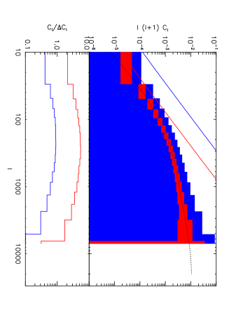
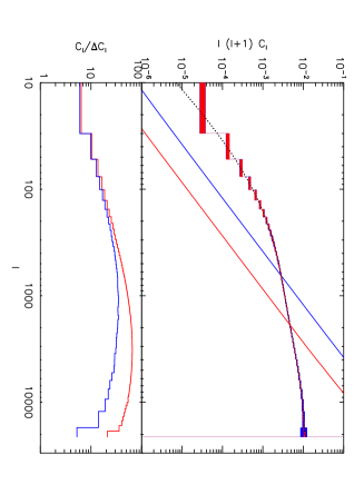
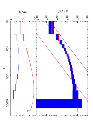
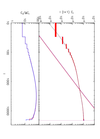
Figure 3 illustrates how uncertainties in the power spectrum estimate depend on the redshift of reionization. We compare results for instantaneous reionization at redshifts of 7 and 10 for 3 years of observation with an SKA-like telescope. When $z_{\rm reion}$ is high, there are fewer independent sources of 21 cm emission in the observable frequency range and the noise goes up significantly. Nevertheless, using only the emission between $z=10$ and 13, a good convergence power spectrum can still be recovered, although mapping the dark matter distribution would no longer be possible. A telescope that goes to lower frequencies could tolerate higher reionization redshifts without such performance degradation. An example is the MWA, although it currently has insufficient collecting area for this project. A LOFAR-like telescope would be unable to obtain a useful power spectrum estimate for $z_{\rm reion}\lower 2.15277pt\hbox{$\;\buildrel>\over{\sim}\;$}9$.

Figure 4 illustrates how the uncertainties depend on the bandwidth. Increasing the bandwidth by a factor of 5 makes little difference to the results. It is assumed here that the statistical properties of the noise and source 21 cm radiation are constant within each band. This result indicates that the correlations between frequency bands when $\delta\nu=1$ MHz are not of relevance since they are fully incorporated when the bandwidth is increased. As discussed before, the estimator is optimized for the case where the statistical properties of the noise and source 21 cm radiation are constant across each band and so it is better to use a smaller bandwidth where this assumption is better justified.

The lensing map of the cosmic mass distribution can have good fidelity while the temperature map of high redshift 21cm emission is noise-dominated on the same scale. This somewhat counter-intuitive situation reflects the fact that it is better to have more independent redshift slices at low signal-to-noise than to make high-quality images of the brightness temperature in a small number of channels.

7.2 Matter power spectrum

Figure 5: Forecast uncertainties in a reconstruction of the matter power spectrum from lensing of high-redshift 21 cm emission for observations with our LOFARII-3yr parameter set. We have taken 7.93 points per decade in the model power spectrum and have used no tomographic information. We assume $f_{\rm sky}=0.25$.

Figure 6: Forecast uncertainties in a reconstruction of the matter power spectrum from lensing of high-redshift 21 cm emission for observations with our SKA-3yr parameter set. We have taken 15.87 points per decade in the model power spectrum and have used no tomographic information. We assume $f_{\rm sky}=0.25$.

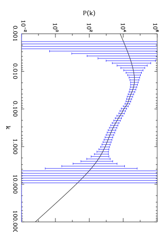
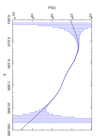
Two-dimensional $\hat{\kappa}(\ell)$ measurements can also be used to estimate the power spectrum of matter fluctuations directly, if the background cosmology (and thus the evolution with redshift of the matter fluctuations) is assumed to be known. To show this, we model the matter power spectrum by linearly interpolating between points that are evenly spaced in $\ln k$. The $\ln P(k)$ values are treated as the model parameters in this case. Equation (31) can then be used to find the expected uncertainties in the power spectrum reconstruction. For this latter calculation we assume purely linear evolution with redshift and fix the shape of the power spectrum to be that given by the CAMB computer code (Lewis et al., 2000).

The uncertainties in these $P(k)$ measurements at different $k$ values will be correlated, and their values will depend on the number of points used to represent the power spectrum – the more points the better the $k$-space resolution, but the larger the noise per point. Figures 5 and 6 show forecast uncertainties for two of our observational parameter sets. The matter power spectrum should be extremely well determined with 3 years of SKA data, and using tomographic information would improve the estimate still further.

The comoving scales which contribute most to 21 cm lensing can be seen clearly in figures 5 and 6. This technique is complementary to CMB fluctuation measurements which probe structure on scales with $10^{-4}<k<0.1$ (Spergel et al., 2007). The scales probed by 21 cm lensing and by galaxy clustering surveys overlap partly, but in the former case the mass is probed directly with no bias uncertainties, and the effective redshift of the measurement is much higher (see the next section) so that uncertainties due to nonlinearities are also reduced. Baryon acoustic oscillations can be seen in the power spectrum in figures 5 and 6 in the range $k=0.04$ – $0.4~{}\mbox{Mpc}^{-1}$. They would be well measured in the SKA-3yr case. These features would provide additional leverage when estimating cosmological parameters, but we do not take this into account in section 7.4 below.

7.3 Tomographic information

Figure 7: The uncorrelated modes in a decomposition of an estimate of the structure growth function for the LOFARII-3yr case. The upper panel shows the redshift dependence of the two modes which are expected to yield estimates with signal-to-noise above 1, while the lower panel gives the signal-to-noise values forecast for the 10 best constrained modes. The $x$-axis is simply the mode number. Corresponding modes are indicated using the same colour in each panel. The growth function is discretized into 20 points spaced evenly in $\log(z)$ and $\kappa(\ell,z_{s})$ are binned into 20 evenly spaced $z_{s}$ bins. We assume $f_{\rm sky}=0.25$.

Figure 8: The uncorrelated modes in a decomposition of an estimate of the structure growth function for the SKA-3yr case. The upper panel shows the redshift dependence of the five modes which are expected to yield estimates with signal-to-noise above 1, while the lower panel gives the signal-to-noise values forecast for the 10 best constrained modes. Corresponding modes are indicated using the same colour in each panel. The growth function is discretized into 50 points spaced evenly in $\log(z)$ and the $\kappa(\ell,z_{s})$ are binned into 20 evenly spaced $z_{s}$ bins. We assume $f_{\rm sky}=0.25$.

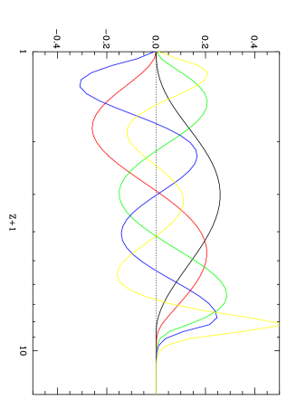
As discussed in section 4, there is tomographic information in the measured $\kappa(\ell,z_{s})$. This makes it possible, in principle, to measure how $P(k)$ evolves with redshift, and so to probe dark energy through its indirect effects on the growth rate of linear fluctuations.

Table 2: Forecast constraints on cosmological parameters for full sky surveys. All constraints scale with sky coverage as $f_{\rm sky}^{-1/2}$ except that the dark energy figure of merit, FOM, scales as $f_{\rm sky}$. The quantities in parentheses are the marginalized uncertainties for constant $w$ ($w_{a}=0$). Both the high redshift 21 cm emission and the lensed galaxy population are assumed to have been binned into ten disjoint redshift intervals when making the corresponding parameter estimates.

		$\ln A$	$n_{s}$	$\Gamma$	$\Omega_{\Lambda}$	$w_{o}$	$w_{a}$	FOM
	assumed values	-9.6 ($\sigma_{8}=0.75$)	1	0.19	0.3	-1.0	0
LOFARII-3yr	marginalized	2.2	0.22	0.11	0.64	3.0 (1.3)	11	0.075
	unmarginalized	0.0047	0.0021	0.00038	0.0025	0.027	0.17
LOFARII-3yr	marginalized	0.036	0.0036	0.0012	0.0060	0.43 (0.053)	1.6	12
+ Planck	unmarginalized	0.0049	0.0016	0.00011	0.00047	0.0066	0.023
LOFARII-3yr	marginalized	0.032	0.0045	0.0017	0.0033	0.028 (0.0087)	0.087	1300
+ galaxies	unmarginalized	0.00032	0.00030	$2.2\times 10^{-5}$	0.00015	0.0011	0.0053
LOFARII-3yr	marginalized	0.0086	0.0033	0.00053	0.0021	0.018 (0.0050)	0.056	3600
+ galaxies + Planck	unmarginalized	0.00034	0.00030	$2.1\times 10^{-5}$	0.00014	0.0011	0.0052
SKA-3yr	marginalized	0.029	0.011	0.0016	0.013	0.044 (0.026)	0.12	310
	unmarginalized	0.00020	0.00023	$1.3\times 10^{-5}$	0.00024	0.0018	0.011
SKA-3yr	marginalized	0.012	0.0036	0.00068	0.0027	0.036 (0.011)	0.12	760
+ Planck	unmarginalized	0.00020	0.00023	$1.3\times 10^{-5}$	0.00022	0.0017	0.0097
SKA-3yr	marginalized	0.017	0.0029	0.00096	0.0022	0.018 (0.0031)	0.054	6000
+ galaxies	unmarginalized	0.00018	0.00019	$1.1\times 10^{-5}$	0.00012	0.00083	0.0039
SKA-3yr	marginalized	0.0074	0.0027	0.00046	0.0017	0.014 (0.0020)	0.046	11000
+ galaxies + Planck	unmarginalized	0.00018	0.00019	$1.1\times 10^{-5}$	0.00012	0.00082	0.0039
galaxy lensing	marginalized	0.045	0.0052	0.0024	0.0036	0.030 (0.010)	0.10	970
	unmarginalized	0.00034	0.00030	$2.2\times 10^{-5}$	0.00015	0.0011	0.0053

While density perturbations are small they grow linearly, $\delta(\boldsymbol{\ell},z)=D_{g}(z)\delta(\boldsymbol{\ell},z=z_{o})/D_{g}(z_{o})$ where $z_{o}$ is some initial redshift. Within General Relativity the linear growth function $D_{g}(z)$ is directly related to the cosmic expansion history $a(z)$ and so through the Friedmann equation to the history of the various contributions to the cosmic energy density. In other theories of gravity $D_{g}(z)$ and $a(z)$ are independent (Peebles, 1980; Bertschinger, 2006). A comparison of precise measurements of the two can thus be used to test Einstein’s theory.

Although structure growth is not precisely linear for all the $\ell$ values and for the full range of redshifts probed by 21 cm lensing, it is probably a good approximation for the modes that are probed with high signal to noise. Without a specific theory for the nature and amount of dark energy the exact form of $D_{g}(z)$ is unknown. In this section we model $D_{g}(z)$ as piecewise linear between a set of interpolation redshifts at which we treat its values as unknown parameters to be estimated. Note that this implies more freedom than is physically allowed, since $D_{g}(z)$ should, for example, decrease smoothly and monotonically with redshift. Technically our approach is not fully self-consistent since the angular size distances in $\kappa(\vec{\ell},z_{s})$ [equation (2)] depend on the cosmic expansion history and so should change when $D_{g}(z)$ changes. Such effects are weaker than those coming from the growth function itself, so we neglect them here. In section 7.4 below, we investigate an alternative approach in which we parameterize the equation of state of dark energy and then use the Friedmann and linear growth equations to calculate its consequences for $a(z)$ and $D_{g}(z)$.

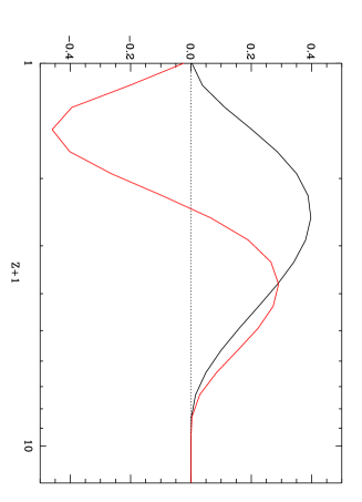
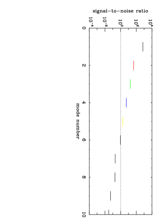
The Fisher matrix for the uncertainties in the estimated values of $D_{i}=D_{g}(z_{i})$ is highly non-diagonal, showing that these parameters cannot all be estimated independently. To understand what properties of the growth function can actually be constrained, it is useful to decompose $D_{g}(z)$ into modes that diagonalize the Fisher matrix, as in equation (20). Figures 7 and 8 show the well constrained modes in such decompositions, together with forecasts of their signal-to-noise ratios for surveys corresponding to our LOFARII-3yr and SKA-3yr cases. We choose the $z_{i}$ to be evenly spaced in $\ln(1+z)$ because we find this to give the best results with the fewest points, but we have tried several other spacings and the results are, as expected, nearly independent of this choice.

In the LOFARII-3yr case (figure 7), estimates for two modes are forecasted to have signal-to-noise above 2. The best measured mode can be interpreted as the normalization of the power spectrum at $z\sim 2$, while the higher order modes measure the rate , acceleration and higher derivatives of structure growth over the redshift range, $z\sim 0.5$ to 4.

In the SKA-3yr case (figure 8), five modes should have amplitude estimates with signal-to-noise greater than 1. It should thus be possible to map the growth function for $z\lower 2.15277pt\hbox{$\;\buildrel>\over{\sim}\;$}0.5$. In standard $\Lambda$CDM $D_{g}(z)$ is characterized by only two parameters, $\Omega_{\rm matter}$ and $\Omega_{\Lambda}$, while four or five could be measured in this way, providing a test of the consistency of this simple model and an opportunity to discover something new.

The complete 3-dimensional density field could also, in principle, be reconstructed. Unlike the case of growth function reconstruction, there is no longer any sample variance, since this part of the “noise” is now the signal. The procedure for doing such reconstructions is described in section 4.1, but we will not investigate it further in this paper since it does not probe the background cosmology directly.

7.4 Cosmological parameters

Within any particular model for dark energy, the standard cosmological parameters can be constrained directly, as described in section 4.2. We here investigate constraints on a set of six parameters $\{\ln A,n_{s},\Gamma,\Omega_{\Lambda},w_{o},w_{a}\}$. $A$ is the dimensionless normalization of the primordial power spectrum and $n_{s}$ is its spectral index. $\Gamma$ is the power spectrum shape parameter (Efstathiou et al., 1992) given by $\Gamma\simeq\Omega_{m}h\exp(-2\Omega_{b})$ (Peacock & Dodds, 1994). The first three parameters only affect the shape and amplitude of the matter power spectrum. The other three determine the expansion history $a(z)$ and the linear growth function $D_{g}(z)$. In this parameterization the lensing results are independent of $H_{o}$ (although the CMB constraints are not) and, as a result, many of the parameter degeneracies which can cause numerical instabilities when inverting the Fisher matrix are avoided. We assume the Universe to be flat, $\Omega_{m}+\Omega_{\Lambda}=1$. This parameter set conforms to that used by the Dark Energy Task Force (DETF) in their investigation of the relative merits of different observational probes of dark energy. The dark energy equation of state parameter is here assumed to evolve as $w(a)\equiv p/\rho=w_{o}+(1-a)w_{a}$, where $a=(1+z)^{-1}$. This is an arbitrary, but useful model that has become popular in the literature.

Table 3: As Table 2 except that the sky coverage of the 21 cm lensing surveys is taken to be 25% and that of the galaxy lensing survey to be 48%.

		$\ln A$	$n_{s}$	$\Gamma$	$\Omega_{\Lambda}$	$w_{o}$	$w_{a}$	FOM
	assumed values	-9.6 ($\sigma_{8}=0.75$)	1	0.19	0.3	-1.0	0
LOFARII-3yr	marginalized	0.052	0.0068	0.0028	0.0049	0.041 (0.013)	0.13	570
+ galaxies	unmarginalized	0.00049	0.00043	$3.2\times 10^{-5}$	0.00021	0.0016	0.0076
SKA-3yr	marginalized	0.029	0.0046	0.0016	0.0036	0.029 (0.0048)	0.091	2300
+ galaxies	unmarginalized	0.00032	0.00032	$2.0\times 10^{-5}$	0.00019	0.0013	0.0064
SKA-3yr	marginalized	0.0098	0.0035	0.00061	0.0022	0.020 (0.0028)	0.064	5600
+ galaxis + Planck	unmarginalized	0.00032	0.00032	$2.0\times 10^{-5}$	0.00018	0.0013	0.0062
galaxies	marginalized	0.065	0.0075	0.0034	0.0053	0.043 (0.014)	0.15	470
	unmarginalized	0.00049	0.00044	$3.2\times 10^{-5}$	0.00021	0.0016	0.0077

Table 2 shows forecasts of the uncertainties in estimates of these parameters both unmarginalized and marginalized over all other parameters in the set. The difference between the marginalized and unmarginalized values indicates the importance of parameter degeneracies. For ease of comparison, these forecasts (unrealistically) assume full sky coverage for the 21 cm and galaxy lensing surveys; the quoted uncertainties scale as $f_{sky}^{-1/2}$ for lower sky coverage accept when CMB constraints are included. The first four parameters are constrained even in the LOFARII-3yr case, but the same is not true for the parameters of the dark energy equation of state. This reflects the fact that, in the model we are assuming, dark energy is insignificant for the growth of structure at $z\lower 2.15277pt\hbox{$\;\buildrel>\over{\sim}\;$}1$, while, as demonstrated in section 7.3, 21 cm lensing is most sensitive to structure growth above $z\sim 1$.

The DETF introduced a figure of merit (FOM) in order to compare the power of different observational techniques to constrain dark energy. The figure of merit is inversely proportional to the area of the error ellipse in the $w_{o}$–$w_{a}$ plane after marginalizing over the other parameters. These values are given in the last column of Table 2.

The parameter degeneracies in 21 cm lensing can be significantly reduced by incorporating information at low redshift from galaxy lensing surveys. The noise in power spectrum estimates from such surveys can be written as $N_{\kappa}(\ell)=\sigma^{2}_{\epsilon}/n_{\rm g}$ where $n_{\rm g}$ is the angular number density of background galaxies and $\sigma_{\epsilon}$ is the root-mean-square intrinsic ellipticity of those galaxies. This neglects all systematic errors as well as photometric redshift uncertainties. The latter can be important for tomographic measurements. Following standard assumptions, we model the redshift distribution of usable galaxies as $\eta(z)\propto z^{2}e^{-(z/z_{o})^{1.5}}$, where $z_{o}$ is set by the desired median redshift, and we adopt $\sigma_{\epsilon}=0.25$. The proposed satellite SNAP is expected to achieve a usable galaxy density of $n_{\rm g}\simeq 100\mbox{ arcmin}^{-2}$ with a median redshift $z\sim 1.23$, but it would only survey $\sim 2\%$ of the sky at this depth. The DUNE mission proposes to survey almost the whole extragalactic sky to a usable density of $n_{\rm g}\simeq 35\mbox{ arcmin}^{-2}$ with a median redshift of $z\sim 0.9$. Several planned ground-based surveys – LSST, PanSTARRS, VISTA will cover comparable areas to DUNE at a similar depth. Since the larger sky coverage more than outweighs the reduced depth when constraining cosmological parameters, we adopt the ”DUNE” parameter set when comparing the power of 21 cm, galaxy, and combined lensing surveys. In order to use tomographic information, we divide the galaxies into 10 redshift bins each containing the same number of galaxies.

We also include the predicted constraints from CMB observations with the Planck Surveyor Satellite. This is done by adding the Fisher matrix for the lensing surveys to the Planck Fisher matrix as calculated in Rassat et al. (2008). The CMB alone puts almost no constraint on $w_{o}$ and $w_{a}$, but the parameter degeneracies in the lensing surveys are greatly reduced by including CMB information. Our lensing Fisher matrix computer code was tested against that of Amara & Refregier (2007) in order to ensure the accuracy of the uncertainties we forecast for parameter estimates.

Table 2 compares the uncertainties forecast for a 21 cm lensing survey alone with those forecast for the galaxy lensing survey alone, and for combinations of surveys. A full-sky 21 cm survey with LOFARII-3yr parameters would not constrain these parameters as well as a full-sky ”DUNE” survey. The full-sky SKA-3yr survey would produce constraints that are similar to the galaxy survey on this parameter set. As noted above, all the action occurs at relatively low redshift for this particular dark energy model. When the two types of surveys are combined they give much tighter constraints than either survey alone. Even the seemingly insensitive LOFARII-like observations can improve the dark energy constraints (a factor of 1.3 in the FOM) when combined with the galaxy survey. Combining a survey with SKA-like sensitivity with a galaxy lensing survey improves the FOM by a factor of $\sim 6$ and when CMB data is included the improvement is more than on order of magnitude.

In practice, 21 cm lensing surveys are not likely to be full-sky, whereas at least half the sky could be covered by a satellite-based galaxy lensing survey (regions at low Galactic latitude are unusable). In Table 3 we combine 21 cm lensing surveys covering 25% of the sky with a galaxy lensing survey covering half the sky and the Planck CMB constraints. Even with this reduced size the combination of the two surveys results in a drastic improvement in the dark energy FOM and in other parameter constraints when compared with any of the surveys by itself.

It is important to recognize that the constraints on dark energy found here for 21 cm surveys alone are in large part a consequence of the particular parameterization adopted for the dark energy equation of state. It could be that the energy density of dark energy is still significant above $z\sim 1$ or that the rate of structure formation is otherwise significantly modified at such redshifts. This is the case in many more physically motivated models, for example, early dark energy models (Ratra & Peebles, 1988; Caldwell et al., 1998), 4-D gravity (Dvali et al., 2000), coupled scalar field theories (Amendola, 2000) and some possible modifications of the underlying theory of gravity (Carroll et al., 2004, for example). In some of these models the growth factor could differ from the standard one by a factor of 2 at $z=2$. Galaxy lensing alone would not able to distinguish between many of these theories, because of the poor leverage it offers on the high redshift Universe. As shown in section 7.3, 21 cm lensing could probe the energy density evolution back to $z\simeq 7$.

8 conclusions

We have shown that a very large amount of cosmological information could be extracted from the gravitational lensing of pregalactic 21 cm radiation. The planned low-frequency radio telescopes, an upgraded LOFAR or SKA, will already have sufficient sensitivity to do this successfully as long as reionization occurs sufficiently late, foreground contamination can be accurately removed, and enough sky can be observed. Under these conditions, the matter power spectrum should be well measured in two and three dimensions, and the growth of structure will be probed from $z=0.5$ to $z=7$. Such observations would constrain many cosmological quantities, in particular the form of the primordial power spectrum and presence of early dark energy, to unprecedented accuracy.

Combining 21 cm lensing surveys with surveys of lensing of foreground galaxies would dramatically improve constraints on structure growth at $z\lower 2.15277pt\hbox{$\;\buildrel<\over{\sim}\;$}1$ where the strongest effects occur in the most popular parameterizations of dark energy. Increasing the collecting area of the telescopes by a factor of $\sim 2$ would also dramatically increase their sensitivity to lensing, as would extending their frequency range to lower values, if foregrounds permit.

Acknowledgments

We would like to thank Adam Amara for allowing use of his own software to compare with results from our own parameter constraint codes. We would like than J. Weller for help in calculating the expected fisher matrix for the Planck satellite mission.

References

- Amara & Refregier (2007) Amara, A. & Refregier, A. 2007, ArXiv e-prints, 710
- Amendola (2000) Amendola, L. 2000, MNRAS, 312, 521
- Bertschinger (2006) Bertschinger, E. 2006, ApJ, 648, 797
- Caldwell et al. (1998) Caldwell, R. R., Dave, R., & Steinhardt, P. J. 1998, Physical Review Letters, 80, 1582
- Carroll et al. (2004) Carroll, S. M., Duvvuri, V., Trodden, M., & Turner, M. S. 2004, Phys.Rev.D, 70, 043528
- Dvali et al. (2000) Dvali, G., Gabadadze, G., & Porrati, M. 2000, Physics Letters B, 485, 208
- Efstathiou et al. (1992) Efstathiou, G., Bond, J. R., & White, S. D. M. 1992, MNRAS, 258, 1P
- Field (1959) Field, G. B. 1959, ApJ, 129, 536
- Furlanetto et al. (2006) Furlanetto, S. R., Oh, S. P., & Briggs, F. H. 2006, Phys.Rep., 433, 181
- Hilbert et al. (2007) Hilbert, S., Metcalf, R. B., & White, S. D. M. 2007, MNRAS, 382, 1494
- Hu & Keeton (2002) Hu, W. & Keeton, C. R. 2002, Phys.Rev.D, 66, 063506
- Hu & Okamoto (2002) Hu, W. & Okamoto, T. 2002, ApJ, 574, 566
- Lewis et al. (2000) Lewis, A., Challinor, A., & Lasenby, A. 2000, ApJ, 538, 473
- Lu & Pen (2007) Lu, T. & Pen, U.-L. 2007, ArXiv e-prints, 710
- Madau et al. (1997) Madau, P., Meiksin, A., & Rees, M. J. 1997, ApJ, 475, 429
- McQuinn et al. (2006) McQuinn, M., Zahn, O., Zaldarriaga, M., Hernquist, L., & Furlanetto, S. R. 2006, ApJ, 653, 815
- Metcalf & White (2007) Metcalf, R. B. & White, S. D. M. 2007, MNRAS, 381, 447
- Morales (2005) Morales, M. F. 2005, ApJ, 619, 678
- Peacock & Dodds (1994) Peacock, J. A. & Dodds, S. J. 1994, MNRAS, 267, 1020
- Peacock & Dodds (1996) —. 1996, MNRAS, 280, L19
- Peebles (1980) Peebles, P. J. E. 1980, The Large-Scale Structure of the Universe (Princeton, NJ: Princeton University Press)
- Rassat et al. (2008) Rassat, A., Amara, A., Amendola, L., Castander, F. J., Kitching, T., Kunz, M., Refregier, A., Wang, Y., & Weller, J. 2008, ArXiv e-prints
- Ratra & Peebles (1988) Ratra, B. & Peebles, P. J. E. 1988, Phys.Rev.D, 37, 3406
- Spergel et al. (2007) Spergel, D. N., Bean, R., Doré, O., Nolta, M. R., Bennett, C. L., Dunkley, J., Hinshaw, G., Jarosik, N., Komatsu, E., Page, L., Peiris, H. V., Verde, L., Halpern, M., Hill, R. S., Kogut, A., Limon, M., Meyer, S. S., Odegard, N., Tucker, G. S., Weiland, J. L., Wollack, E., & Wright, E. L. 2007, ApJ Sup., 170, 377
- Takada & Jain (2004) Takada, M. & Jain, B. 2004, MNRAS, 348, 897
- Vale & White (2003) Vale, C. & White, M. 2003, ApJ, 592, 699
- Zahn & Zaldarriaga (2006) Zahn, O. & Zaldarriaga, M. 2006, ApJ, 653, 922
- Zaldarriaga et al. (2004) Zaldarriaga, M., Furlanetto, S. R., & Hernquist, L. 2004, ApJ, 608, 622