Metallicity and Physical Conditions in the Magellanic Bridge

Abstract

We present a new analysis of the diffuse gas in the Magellanic Bridge (RA $\gtrsim 3^{\rm h}$) based on HST/STIS E140M and FUSE spectra of 2 early-type stars lying within the Bridge and a QSO behind it. We derive the column densities of H I (from Ly $\alpha$), N I, O I, Ar I, Si II, S II, and Fe II of the gas in the Bridge. Using the atomic species, we determine the first gas-phase metallicity of the Magellanic Bridge, $[{\rm Z/H}]=-1.02\pm 0.07$ toward one sightline, and $-1.7<[{\rm Z/H}]<-0.9$ toward the other one, a factor 2 or more smaller than the present-day SMC metallicity. Using the metallicity and $N($H I$)$, we show that the Bridge gas along our three lines of sight is $\sim$70–90% ionized, despite high H I columns, $\log N($H I$)\simeq 19.6$–20.1. Possible sources for the ongoing ionization are certainly the hot stars within the Bridge, hot gas (revealed by O VI absorption), and leaking photons from the SMC and LMC. From the analysis of C II*, we deduce that the overall density of the Bridge must be low ($<0.03$–0.1 cm^-3). We argue that our findings combined with other recent observational results should motivate new models of the evolution of the SMC-LMC-Galaxy system.

1. Introduction

The evolution of galaxies is closely coupled to the interactions between them. Encounters between galaxies are frequent and were certainly habitual in the early epoch of galaxy formation (e.g., Barnes & Hernquist, 1992; Larson & Tinsley, 1978; Maller et al., 2006). These encounters reshape the galaxies and transfer mass, energy, metals between the galaxies, and may even create new sites of star formation within the newly produced gaseous features between the galaxies or new burst of star-formations in the colliding galaxies (Larson & Tinsley, 1978; Barton et al., 2007; de Mello et al., 2007). These galactic interactions are not believed to be a major contributor to the pollution of the intergalactic medium (e.g., Aguirre et al., 2001), but they nonetheless affect the metal content and physics of the galaxies themselves and their halos, and therefore the evolution of the galaxies and their surroundings.

In our galactic neighborhood, interactions between the Magellanic clouds and the Galaxy are believed to have produced several large gaseous features: The Magellanic Bridge linking the Small Magellanic Cloud (SMC) and the Large Magellanic Cloud (LMC), the Magellanic Stream and the Leading Arm apparenly linking the Clouds and our Galaxy (e.g., Mathewson et al., 1974; Putman, 2000; Brüns et al., 2005). The Magellanic Bridge is believed to have been produced through an interaction between the SMC and LMC, while the Stream and Leading arm may have arisen through an interaction between the Galaxy and the Clouds (e.g. Gardiner & Noguchi, 1996), although the origin of these latter gaseous features is far from settled (Nidever et al., 2007; Besla et al., 2007). The proximity of these gaseous features and the global view of the Magellanic System with little line-of-sight confusion allow us to study the result of interacting galaxies in a way not otherwise possible. The Magellanic Bridge (hereafter Bridge) is the focus of the present work.

In the past few years, multi-wavelength observations of the Bridge have revealed some key characteristics. Radio H I observations have shown that approximately 2/3 of the H I gas surrounding the Clouds is found in the Magellanic Bridge, while only 25% and 6% are found in the Stream and the Leading Arm, respectively (Brüns et al., 2005). Some of the Bridge gas appears even to build-up and feed the Stream via an Interface Region (Brüns et al., 2005). Far-ultraviolet observations have shown multiple gas phases in the Bridge including not only the well known neutral gas, but also a significant amount of ionized gas and a small H₂ content (Lehner et al., 2001; Lehner, 2002, this paper). Dense molecular clouds were also subsequently identified in form of CO (Muller et al., 2003; Mizuno et al., 2006) (although these CO surveys were realized in the SMC Wing, a much denser region in stars and gas content of the Bridge). Optical studies have revealed massive hot stars throughout the Bridge (Demers & Battinelli, 1998). The ages of these stars are $\sim$10 to 40 Myr, implying that star formation is ongoing within the Bridge gas since these stars could not migrate from the SMC during their lifetimes, although Harris (2007) suggests that star formation in the Bridge may have been more important 200–300 Myr ago.

The N-body numerical simulation of the Galaxy-SMC-LMC system by Gardiner & Noguchi (1996) have reproduced some of the observed characterics of the Bridge (principally the H I column density and velocity distributions), along with those of the Stream. In this paper, we still use their numerical simulation as a basis, although we note that the hypotheses and validity of this model and other recent numerical simulations (e.g., Yoshizawa & Noguchi, 2003) has been put recently in question in view of the new Hubble Space Telescope (HST) measurements of the proper motions of the LMC and SMC (Kallivayalil et al., 2006a, b; Besla et al., 2007, and see §5.3). Gardiner & Noguchi’s model predicts that the Bridge was formed from tidally-stripped gas pulled from the SMC during a close encounter between the SMC and the LMC some 200 Myr ago. The new calculations of the LMC and SMC orbits still suggest that the closest approach between these two galaxies occured some 200 Myr ago (Kallivayalil et al., 2006a), and therefore the new proper motions may only affect the interpretation of the origins of the Stream and Leading Arm. Nevertheless, there appear to be some challenges to these models.

Tidal models predict that both gas and stars are pulled from the SMC, and yet search for an old stellar population in the Bridge has so far failed (Harris, 2007). Furthermore, material pulled from the SMC should have a somewhat similar metallicity that the SMC some 200 Myr ago. But this appears in conflict with the B-type star abundances in the Bridge that imply an extremely low Bridge metallicity, $-1.1$ dex from solar (Rolleston et al., 1999; Lee et al., 2005), a factor of 3 and 5 metal deficiency with respect to the SMC and LMC, respectively. The metallicity in the sparse regions of the Bridge is also at odds with those measured in the SMC wing, also known as the Western end of the Bridge, where the metallicity of B-type stars is found to be SMC-like (Lee et al., 2005). These metallicity estimates complicate the origin of the Bridge and suggest different evolutions or origins for the sparse and dense stellar regions of the Bridge.

An estimate of the present-day metallicy of the Bridge that is independent of stellar measurements is therefore critical. In this work, we present an estimate of the absolute gas-phase abundances of the Bridge toward two stars situated in relatively low H I column density regions. We compare the column densities of the neutral species (N I, O I, Ar I) observed in absorption in the Space Telescope Imaging Spectrograph (STIS) and Far Ultraviolet Spectroscopic Explorer (FUSE) spectra to those for H I Ly$\alpha$ lines toward two early-type stars, i.e. our metallicity estimate is mostly independent of ionization correction. The Bridge Ly$\alpha$ absorption is heavily blended with the Galactic component, but we show that it is feasible to retrieve the Bridge H I column density. Using the metallicity and the amount of H I along these sightlines, we can for the first time quantify the amount of ionized gas in the Bridge; ionized gas is revealed to be a major component of the Bridge, yet this gas-phase is mostly ignored in numerical simulations.

Our paper is organized as follows. In §2 we briefly discuss the previous STIS and FUSE observations, and the new FUSE observations of DGIK 975 and DI 1388. In §3 we discuss our measurements of the metals and the H I colum densities. We present in §4 the first metallicity estimate of the Bridge gas and the fraction of neutral, ionized, and molecular gas. From the C II* diagnostic, we estimate the electron density and cooling rate in the Bridge. In §5 we discuss our results (in particular address the possible origins for the low metallicity and ionization sources of Bridge) and the current observational challenges to numerical simulations. Finally, in §6 we summarize our key findings.

2. Observations

In Fig. 1 we show the locations of our targets on an H I map of the Magellanic System from Brüns et al. (2005) (more properties about the stars can be found in Lehner 2002). DI 1388 and PKS 0312–77 are situated approximately midway between the SMC and LMC, and DGIK 975 lies at the eastern end of the Bridge near the LMC halo, allowing us to probe different regions of the Bridge (see Fig. 1). All these sightlines are outside the SMC Wing that is approximately delimited by the box in Fig. 1.

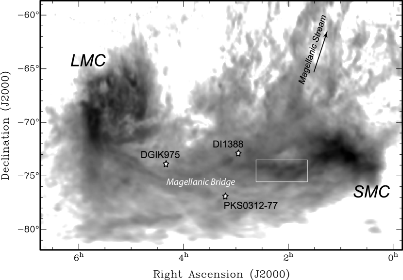
Figure 1.— Location of our targets superimposed on the H I column density distribution from Brüns et al. (2005) (darker regions represent higher $N($H I$)$, see Brüns et al. for the detailed $N($H I$)$ scale). Our sightlines and major features of the Magellanic system are indicated. The box highlights a region known as the SMC Wing or Western end of the Magellanic Bridge.

The two stars were observed with FUSE, HST/STIS E140M, and the Anglo-Australian 3.9-m telescope (AAT). The QSO PKS 0312–77 was observed with STIS E140M and FUSE, but the STIS and FUSE data are of too poor quality for a detailed metal-line absorption analysis. Unfortunately, the FUSE program F018 (PI: Lehner) to obtain a good quality FUV spectrum of this QSO was not completed before the failure of FUSE and only 16% of the requested time was observed. However, the STIS data can be rebinned and used to study the Ly$\alpha$ absorption. For the STIS E140M and AAT observations of DGIK 975 and DI 1388, we refer the reader to Lehner et al. (2001) and Lehner (2002). The previous FUSE observations of these two stars are also described in Lehner (2002). New FUSE observations were obtained for DI 1388 (program U106 non-proprietary re-observations of science targets) and DGIK 975 (program G050, PI: Lehner), adding another 10 ks and 29 ks exposure time, respectively. (Note that the total time for the program U106 is 30 ks, but about half the exposures have no signal.) The total FUSE exposure times are therefore 28 ks for DI 1388 and 52 ks for DGIK 975.

All the FUSE data were recalibrated using the newest calfuse version (v3.2, Dixon et al. 2007). The extracted spectra associated with the separate exposures were aligned by cross-correlating the positions of absorption lines, and then co-added. The oversampled FUSE spectra were binned to a bin size of 0.027 Å (4 pixels), providing about three samples per $\sim$20 ${\rm km\,s}^{-1}$ resolution element. In order to achieve the optimum signal-to-noise, segments with overlapping wavelengths were coadded for the DGIK 975 FUSE spectra. However, we ensured before coadding the various spectra that none of the absorption lines of interest was affected by fixed-pattern noise, by comparing the interstellar profiles in multiple detector segments. The zero point in the final FUSE wavelength scale was established by shifting the average FUSE velocity to the STIS 140M velocity of the same species (e.g., O I, N I, Fe II). STIS data reductions provide an excellent wavelength calibration, with a velocity uncertainty of $\sim$1 ${\rm km\,s}^{-1}$.

3. Analysis

3.1. Metals

The continuum levels near the metal absorption lines were modeled by fitting Legendre polynomials within about $[-300,600]$ ${\rm km\,s}^{-1}$ of each absorption line. Low-order polynomials were generally adopted, but in some cases high-order polynomials were necessary (e.g. Fe III is blended with the stellar photospheric and wind lines). For weak lines, several continuum placements were tested to be certain that the continuum error was robust (see Sembach & Savage, 1992). In Figs. 2 and 3, we show the normalized spectra for the interstellar metal-line transitions in DI 1388 and DGIK 975, respectively (see also Lehner et al., 2001; Lehner, 2002). Selected transitions have no serious blends with other features.

In order to estimate the column density we adopted the apparent optical depth (AOD) method of Savage & Sembach (1991). In this method the absorption profiles are converted into apparent column densities per unit velocity $N_{a}(v)=3.768\times 10^{14}\ln[F_{c}/F_{\rm obs}(v)]/(f\lambda)$ cm^-2 (${\rm km\,s}^{-1}$)^-1, where $F_{c}$ is the continuum flux, $F_{\rm obs}(v)$ is the observed flux as a function of velocity, $f$ is the oscillator strength of the absorption and $\lambda$ is in Å (atomic parameters were adopted from Morton 2003). The total column density was obtained by integrating over the absorption profile $N_{a}=\int N_{a}(v)dv$. According to Savage & Sembach (1991), this method is adequate for data with $b_{\rm line}\gtrsim 0.25$–$0.50b_{\rm inst}$, where $b_{\rm line}$ is the intrinsic $b$-value of the line and $b_{\rm instr}$ is the $b$-value of the instrument. Since $b\equiv$ FWHM$/1.667$, for STIS E140M, $b_{\rm inst}\simeq 4$ ${\rm km\,s}^{-1}$ and for FUSE, $b_{\rm inst}\approx 12$ ${\rm km\,s}^{-1}$. Therefore, we assume that a negligible fraction of the gas has $b\ll 1$ ${\rm km\,s}^{-1}$, an assumption made implicitly in most ISM abundance analyses using these instruments. Yet, we note that if the apparent column densities of a species with similar transitions estimated by both intruments are similar, this implies that there must be little or no unresolved saturation.

The reader should be aware that signatures of cold gas in the Bridge have been found toward DI 1388 and PKS 0312–77. The fraction of cold gas with respect to the warmer gas is unknown. We note that Lehner (2002) derived $b\simeq 2.6$ ${\rm km\,s}^{-1}$ for the H₂ in the Bridge toward DI 1388 using a curve of growth with a single component. If a typical temperature of the molecular gas is $T\sim 100$–200 K, turbulent motions would dominate the broadening of the H₂ lines. Hence even though there may be cold gas, turbulent motions may be important enough to keep the broadening of the atomic and ionic lines greater than 1 ${\rm km\,s}^{-1}$. Because the investigated gas is multiphase (Lehner et al., 2001; Lehner, 2002), the AOD method is favored over the curve-of-growth (COG) or profile fitting methods because the AOD does not make any a priori on the kinematical distribution of the gas along the sightline. Finally, we note that our estimates are also based on non-detection of a line: these strict limits are consistent with our AOD estimates (see below), given us confidence in the results presented here.

When $\tau_{a}\ll 1$ (which is the case for several transitions used in this work), unresolved saturation should not be problematic as long as $b$ is not much smaller than 1 ${\rm km\,s}^{-1}$. For stronger lines, unresolved saturated structure can be identified by comparing the lines of the same species with different $f\lambda$ . Following Savage & Sembach (1991), the difference in $f\lambda$ must be a factor of 2 (or 0.3 dex) or more to be able to detect unresolved saturation. The $f\lambda$ values are summarized in Table 1. If some moderate saturation exists, we can correct for it using the procedure described in Savage & Sembach (1991). For various cases of blending and line broadening, they found a tight relation between the difference of the true column density and the apparent column density of the weaker line versus the difference of the strong line and weak line apparent column densities. The correction to the apparent column density of the weak line for a given difference between the strong- and weak-line apparent column densities are summarized in their Table 4.

In cases where we have only reliable information on a single line, we only quote a lower limit on the apparent column density. However, we note that due to the low metallicity of the Bridge, the peak apparent optical depths of metal lines are generally less than 1. Even strong transitions such as O I $\lambda$1302 and N II $\lambda$1083, which have line profiles that are usually completely saturated in the diffuse gas of Galactic or SMC/LMC environments with similar H I column densities, do not reach zero flux (at least toward DI 1388).

When no absorption is observed for a given species, we measured the equivalent width (and $1\sigma$ error) over the same velocity range found from similar species that are detected. The 3$\sigma$ upper limit on the equivalent width is defined as the 1$\sigma$ error times three. The 3$\sigma$ upper limit on the column density was then derived assuming the absorption line lies on the linear part of the curve of the growth.

Table 1Apparent Column Densities of the Metals

Species	$\lambda$	$\log f\lambda$	$\log N_{a}$
	(Å)
DI 1388
O I	1302.168	1.795	$(>)14.77\pm 0.03$
O I	1039.230	0.974	$(>)14.97\pm 0.06$
O I	950.885	0.176	$15.33\pm 0.10$
O I	936.630	0.534	$15.26\,^{+0.13}_{-0.16}$
O I	924.950	0.154	$15.32\pm 0.13$
N I	1200.710	1.715	$(>)14.07\pm 0.04$
N I	1200.223	2.018	$(>)13.89\pm 0.04$
N I	1134.980	1.674	$(>)14.00\pm 0.08$
N I	964.626	0.882	$(\leq)14.32\,^{+0.13}_{-0.20}$
N I	954.104	0.582	$<14.45$
Ar I	1066.660	1.857	$<13.17$
Ar I	1048.220	2.440	$12.80\pm 0.15$a
Si II	1526.707	2.308	$14.14\pm 0.07$
Si II	1304.370	2.051	$14.18\pm 0.02$
S II	1253.805	1.136	$14.25\pm 0.10$
S II	1250.578	0.832	$14.27\pm 0.07$
Fe II	1608.451	1.970	$13.95\pm 0.02$
Fe II	1144.939	1.980	$13.93\pm 0.05$
Fe II	1143.226	1.341	$13.95\pm 0.10$
Fe II	1055.262	0.812	$(\leq)14.05\,^{+0.15}_{-0.25}$
DGIK 975
O I	1039.230	0.974	$(>)15.20\pm 0.04$
N I	1134.980	1.674	$(\leq)13.88\,^{+0.12}_{-0.16}$
Ar I	1048.220	2.440	$<12.92$
Si II	1020.699	1.225	$(\leq)14.54\,^{+0.14}_{-0.20}$
Fe II	1144.939	1.980	$14.18\pm 0.03$
Fe II	1143.226	1.341	$14.36\pm 0.07$
Fe II	1125.448	1.245	$14.44\pm 0.10$
Fe II	1093.877	1.555	$14.34\pm 0.05$
Fe II	1055.262	0.812	$(\leq)14.60\,^{+0.10}_{-0.16}$

Note. — Atomic parameters are from Morton (2003). $N_{a}$ is the apparent column density in cm^-2, except when the “$(<)$” sign is present, which is a 3$\sigma$ upper limit; “$(\leq)$ indicates that the detection is barely 3$\sigma$, and “$(>)$” indicates that the line is likely saturated (see text for more details). $a$: We note that Lehner (2002) found a column density twice smaller for Ar I. N. Lehner revisited the original reduced data (calfuse v2.0.5) and concludes that the measurement was made using solely LiF 1A, which appears to suffer from fixed-pattern noise contamination (see Fig. 2 in Lehner 2002) but has been corrected with the new calibration. Indeed the LiF 1A and LiF 2B segments reduced with calfuse v3.2 give consistent results, and those are consistent with $N($Ar I$)$ determined with LiF 2B calfuse v2.0.5 data.

Figure 2.— Normalized profiles against the LSR velocity near the Bridge velocities of neutral and singly ionized species in the STIS E140M and FUSE spectra of DI 1388. The Bridge absorption occurs between about 160 and 220 ${\rm km\,s}^{-1}$ toward this line of sight. The “x” shows part of the spectrum that is contaminated by other absorbing features.

Figure 3.— Normalized profiles against the LSR velocity near the Bridge velocities of neutral and singly ionized species in the STIS E140M and FUSE spectra of DGIK 975. The Bridge absorption occurs between about 100 and 200 ${\rm km\,s}^{-1}$ toward this line of sight. The “x” shows part of the spectrum that is contaminated by other absorbing features.

In Table 1, we present our estimates of the apparent column densities for DI 1388 and DGIK 975. Below, we review each sightline separately:

DI 1388: In Table 1, we present our raw measurements of the apparent column densities for DI 1388. Each considered species have at least 2 transitions with $\Delta\log(f\lambda)\gtrsim 0.3$.
Singly-ionized species: In Fig. 4, we show the apparent column density profiles of Si II $\lambda$$\lambda$1304, 1526 and the integrated column densities agree remarkably well, especially at $\sim$198 ${\rm km\,s}^{-1}$ where the absorption is the strongest. The continuum near Si II $\lambda$1526 is somewhat more complicated than for Si II $\lambda$1304, which results in a larger uncertainty. A similar agreemeent is found for S II, although we note that the continuum near the blue side of S II $\lambda$1253 is more complicated. For Fe II, the data are from FUSE and STIS. There is again an excellent agreement between the weak and strong transisitions. Furthermore, Fe II $\lambda$$\lambda$1608 (STIS), 1144 (FUSE) have similar strengths and apparent column densities. Therefore the coarser spectral resolution of FUSE does not seem to affect our apparent column estimates. Hence for the singly-ionized species, there is no evidence of saturation for the lines summarized in Table 1.

Ar I: The transition at 1066.66 Å is a 3$\sigma$ upper limit. This is a firm upper limit irrespective of the intrinsic broadening of the line. Ar I $\lambda$1048 is detected and its apparent column density is consistent with the weaker transition. If the strong transition has some unresolved saturation, it is likely less that 0.1 dex.

N I: The transitions at 1200.71 and 1134.98 Å have similar strengths, but the agreement in the $N_{a}$ of these two lines is not as good as for Fe II, even though the $N_{a}$ estimates of these two lines overlap within 1$\sigma$. This suggests that there may be some unresolved saturation. The apparent column density of N I $\lambda$1200.22 is 0.18 dex smaller than N I $\lambda$1200.711 (see also Fig. 4). Therefore $N_{a}($N I $\lambda$1200.711$)$ needs to be corrected for saturation. Using the results of Savage & Sembach (1991), we find that the correction is 0.27 dex. The corrected column density of N I is therefore $\log N($N I$)=14.34\pm 0.08$ (where the errors include statistical and saturation correction uncertainties). This result can be directly tested with the weak N I $\lambda$964 transition, a 2.8–3.1$\sigma$ dectection, which yields $\log N_{a}=14.32\,^{+0.13}_{-0.20}$ dex, in excellent agreement with our above corrected column density (note that this N I line has a similar strength to O I $\lambda$924 described below but the continuum placement is much more straightforward for the O I line, explaining the difference in the errors). The upper limit on N I $\lambda$954 is also consistent with our estimate.

O I: The strong transitions at 1302.17 and 1039.23 Å give much smaller apparent column densities than the weak lines, and are therefore saturated. There are also two weak transitions at 924.95 and 950.89 Å that are 3.0–3.2$\sigma$ and 4.2–4.5$\sigma$ detections, respectively. Near the weakest transitions O I $\lambda$924 there is a contaminating feature on the blue side of the line, while there is a very weak contaminant on the red side of O I $\lambda$950 (see Fig. 2). However, the apparent column densities of O I $\lambda$924 and $\lambda$950 are consistent with each other. We also tested this by measuring half the O I $\lambda$924 profile known to be free of contamination and the resulting $N_{a}\times 2$ is consistent with the value reported in Table 1. The continua near these lines are well modeled with a straight line. O I $\lambda$$\lambda$924,950 have $\tau_{a}\ll 1$ and similar $f\lambda$. O I $\lambda$936 is about 0.3 dex stronger than these lines and can be used to test for any unresolved structures. However, this line is partially blended with H I $\lambda$937, complicating the continuum placement, which results in a larger error. Within the errors, the apparent column densities of the three lines are consistent. Nevertheless, to be cautious, we adopted the weighted average of the apparent column densities of O I $\lambda$$\lambda$924,950 and added an error in quadrature of $+$0.07 dex to include any possible weak saturation. Our adopted O I column density is $\log N($O I$)=15.33\,^{+0.11}_{-0.08}$.

DGIK 975: The STIS data are of lower quality than those for the DI 1388 and the peak apparent optical depths are greater than 1 for all the detected species (see Fig. 3). We therefore use only the FUSE data. Unfortunately, the FUSE stellar spectrum is not as well behaved as the one of DI 1388, and we often have to rely on a single line. Stellar contamination and amount of H I  are more important (see §3.2), so that none of the weak O I and N I lines can be used. The $\lambda$1039 transition is the only available O I line and is likely saturated, providing a firm lower limit. (The apparent column density of O I $\lambda$ cannot be estimated because the signal-to-noise is too low and its absorption reaches zero-flux). Ar I $\lambda$1048 is not detected and provides a firm 3$\sigma$ upper limit. N I $\lambda$1134 is a $2.8$–$3.2\sigma$ detection, and therefore the estimate of the apparent column should be considered as an upper limit. The same applies for Si II $\lambda$1020 (the measurement of this line being complicated by the uncertain continuum placement). Only for Fe II, several transitions can be measured. Following the above method, we estimate the average column density using the weak lines (i.e. excluding Fe II $\lambda$1144), and add a systematic error to take into account possible unresolved structures.

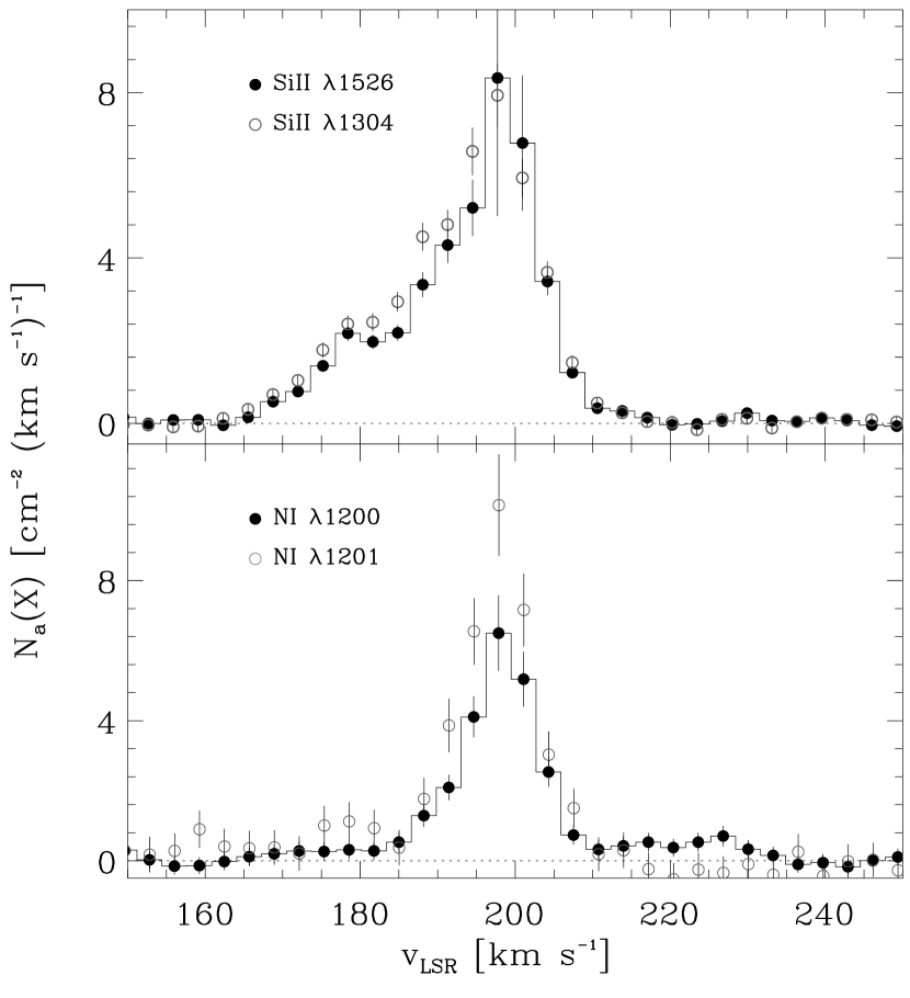
Figure 4.— Comparison of the apparent column density profiles for Si II and N I for the DI 1388 sightline. The Si II lines are essentially fully resolved while N I shows some unresolved saturation.

Table 2Adopted column densities of the Metals

Species	$\log N$
DI 1388
O I	$15.33\,^{+0.11}_{-0.08}$
N I	$14.34\pm 0.08$
Ar I	$12.80\pm 0.15$
Si II	$14.17\pm 0.02$
S II	$14.26\pm 0.06$
Fe II	$13.95\pm 0.02$
DGIK 975
O I	$>15.20$
N I	$\leq 13.88\,^{+0.12}_{-0.16}$
Ar I	$<12.92$
Si II	$\leq 14.54\,^{+0.14}_{-0.20}$
Fe II	$14.38\,^{+0.12}_{-0.05}$

Note. — See §3.1 for more details.

Our adopted column densities for neutral and singly-ionized species are summarized in Table 2. There is an overall agreement with previous column density estimates (Lehner et al., 2001; Lehner, 2002), in particular if in Lehner (2002) the O I and N I column densities estimated in the DI 1388 spectrum are systematically smaller than presently, they nonetheless overlap within $1.5\sigma$. The main difference is that he relies on a single-component curve-of-growth analysis using both weak and strong lines, which depends on an assumed velocity distribution that is likely more complex than one Gaussian component. We believe using the AOD method is a better approach to determine the most reliable column densities and errors in view of the complexity of the velocity distribution in these sightlines.

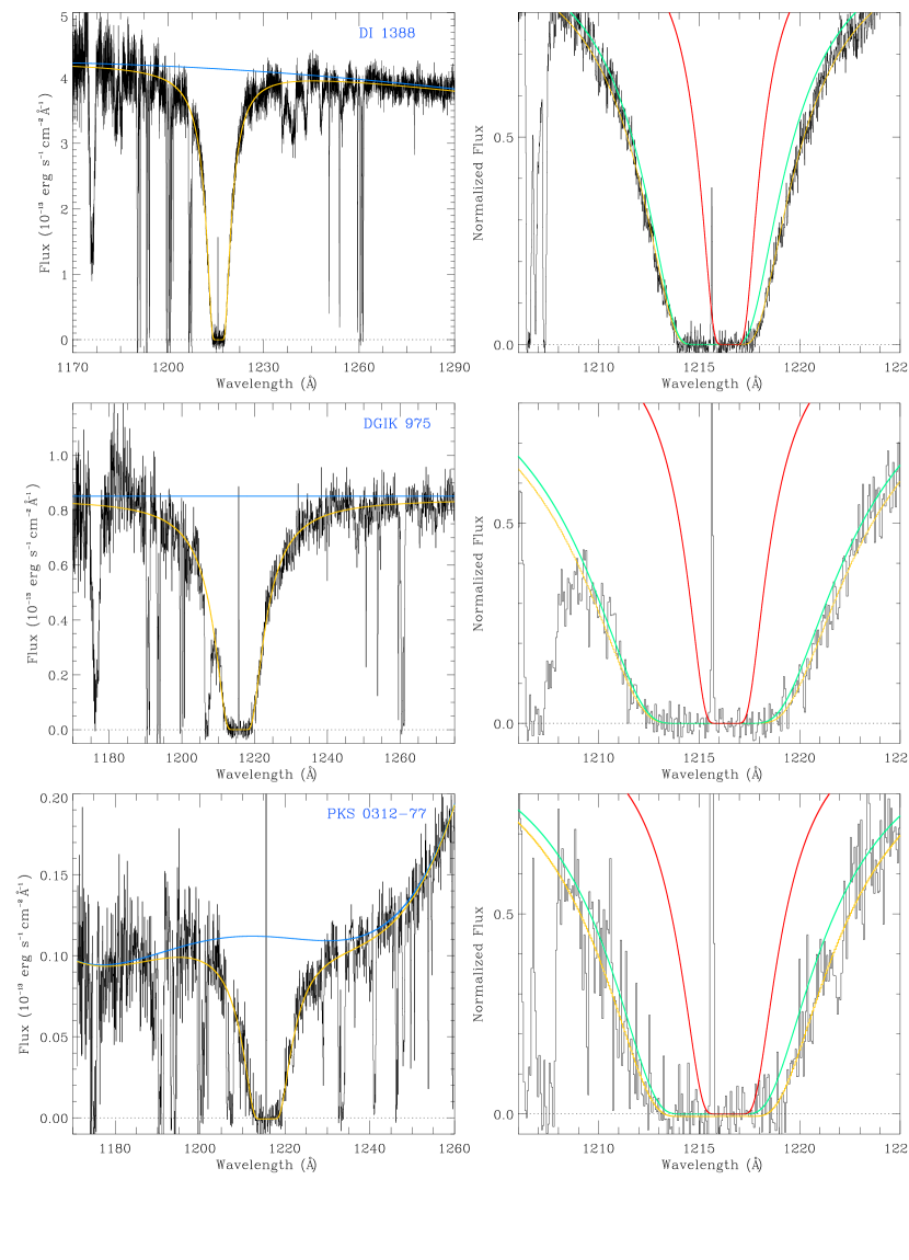
Figure 5.— Left panels: The Ly $\alpha$ profiles in the STIS E140M spectra of DI 1388 (top), DGIK 975 (middle), and PKS 0312–77 (bottom). The blue line shows the continuum and the yellow is the two-component fit to the interstellar Ly $\alpha$ profile. Right panels: A zoom in on the core of the normalized Ly $\alpha$ profiles is shown for each line of sight. The yellow line is the two-component fit, while the green and red lines show only the Galactic and Bridge components, respectively.

3.2. Neutral Hydrogen

Table 3H I Column Density

Sightline/	$v_{\rm LSR}$	$\log N$	$\log N^{\star}$	$\log N_{\rm f}$
Component	(${\rm km\,s}^{-1}$)
DI 1388 G	$-5$	$20.41\pm 0.02$	$\cdots$	$20.41\pm 0.02$
DI 1388 B	$195$	$19.67\pm 0.07$	$18.58$	$19.63\pm 0.07$
DGIK 975 G	$-5$	$20.95\pm 0.08$	$\cdots$	$20.95\pm 0.08$
DGIK 975 B	$160$	$19.95\pm 0.30$	$18.98$	$19.90\pm 0.30$
PKS 0312–77 G	$5$	$20.78\pm 0.06$	$\cdots$	$20.78\pm 0.06$
PKS 0312–77 B	$210$	$20.12\pm 0.30$	$\cdots$	$20.12\pm 0.30$

Note. — “G”: Galactic component; “B”: Bridge component The LSR velocities are fixed and are estimated from the O I absorption profiles. $N$ is the observed column density, $N^{\star}$ is the estimated stellar H I contribution for the H$\beta$ profiles (see text for more details), and $N_{\rm f}$ was corrected for the stellar component in the Bridge component. Note that the errors include different choices of continuum placement and polynomial degree for the continuum, and velocity shifts of $\pm 5$ ${\rm km\,s}^{-1}$.

Here we discuss our derivation of the Bridge H I column based on the analysis of the Ly $\alpha$ absorption. The H I column density is more complicated to derive because both the Galaxy and Bridge contribute to the absorption. H I 21-cm emission observations toward the stars are of little use for the Bridge component because the stars are embedded in the Bridge with an unknown depth. We therefore need to derive $N($H I$)$ from the Ly $\alpha$ absorption. To do so, we fit each damped Ly $\alpha$ absorption line profile with two components that correspond to the Galactic and Magellanic Bridge components. The blue-ward wing of the profile is due primarily to the Galactic component, but the Galactic component cannot completely account for the absorption in the red-ward wing, indicating the need for a Bridge component. By fixing the velocities of the Galactic and Bridge components, we can determine the H I column densities. We note that the amount of H I gas between the Galaxy and the Bridge is negligible, since the H I 21-cm data do not show any emission toward these two lines of sight at a level of $10^{18.3}$ cm^-2, too small to affect the damping wings of Ly $\alpha$. O I is the best metal proxy for H I since its ionization potential and charge exchange reactions with hydrogen ensure that the ionization of H I and O I are strongly coupled. We can therefore use the kinematics of O I to infer those for H I. While the O I profiles show multiple structures in both the Galactic and Bridge components, we only use the average velocities to fix the values for each component. These are listed in Table 3. Below we detail our fitting results for each star.

DI 1388: This line of sight is our best case because the continuum of the star is well behaved and the Galactic H I column density is not so large that it fills the absorption in the red part of the Ly $\alpha$ profile to a large degree. In Fig. 5, we show the profile of Ly $\alpha$ with its continuum and the fit with the two components (top-left panel). On the top-right panel, we show part of the normalized Ly $\alpha$ profile with the two-component fit in yellow, in red the Bridge component, and in green the Milky Way component. This shows that while the Galactic component nearly fits the blue part of the Ly $\alpha$ absorption, there is extra absorption in the red part that is missed by the Galactic component. In Table 3, we summarize the derived column density for each component in the third column. To test the robustness of our fit, we undertook many simulations where the velocity centroids were changed by $\pm 5$ ${\rm km\,s}^{-1}$, the placement of the continuum was varied, and the continuum was modeled by a range of polynomials of degree of 1 to 4. The errors reported in Table 3 were estimated to reflect the 1$\sigma$ distribution between all the trials.

DGIK 975: This line of sight is more complicated because the Galactic H I component is much stronger than toward DI 1388. For the latter, the Galactic H I component is about a factor 5 stronger than the Bridge component, while toward DGIK 975, we found the Galactic component is $\sim$10 times stronger than that of the Bridge. The Si III $\lambda$1206 line is also very strong and removes some information in the blue part of the Ly $\alpha$ absorption. Finally the STIS E140M DGIK 975 spectrum has a much lower S/N; we therefore rebinned these data by 5 pixels before fitting. In Fig. 5, we show our resulting best fit overplotted on the Ly $\alpha$ profile (middle-left panel), where the continuum is well behaved and can be modeled by a straight line. The normalized profile (middle-right panel) indeed shows that the difference between the two-component fit and the single Galactic component fit is small, which results in a large error in $N($H I$)$ of the Bridge feature. However, as for DI 1388, at $1219\lesssim\lambda\lesssim 1222$ Å, where the optical depth is more important, the Galactic component does not properly fit the red part of the absorption without the Bridge component. We also undertook several trials in order to derive the 1$\sigma$ error reported in Table 3.

The H I 21-cm emission data can help to evaluate the solution from our fits, at least for the Galactic component; indeed, since the whole column of Galactic gas is probed in both emission and absorption toward the stars, the infered column densities derived from absorption and emission spectra can be compared. The main uncertainty that arises from such a comparison is that the beam that collected the H I 21 cm emission data is much larger than the pencil-like beam of the absorption observations. Therefore the beam of the radio telescope only represents an average column density of the region near the line-of-sight. Wakker et al. (2001) studied this effect for low-, intermediate-, and high-velocity clouds by comparing $N($H I$)$ measured via a beam of 36′, 9′, 1′, and through Ly $\alpha$ absorption. They found that the “beam-effect” was less important for the low-velocity gas where the range of ratio of $N($H I$)$ measured with a 9′ versus a 36′ is 0.9 to 1.4 than for the HVCs where the range of ratio is 0.3 to 2.1. This difference is because the physical sizes probed by the H I 21 cm data are naturally smaller in nearby gas and therefore less likely to have large angular/spatial variations. Hence H I 21-cm emission observations observed through a 15′ beam should provide reliable $N($H I$)$ within a beam error of about $\pm 0.10$ dex (see also Lehner et al. 2004) for the low-velocity Galactic gas that can be compared to the results from the profile fitting of the Ly $\alpha$ absorption.

With H I 21-cm emission observations from the Parkes 64 m radio telescope with a 15′ beam and 1 ${\rm km\,s}^{-1}$ spectral resolution (M.E. Putman, 1999, private communication) we derive the H I column density for the Galactic component where we make the usual assumption that the medium is optically thin: $\log N($H I$)=20.44\pm 0.11$ toward DI 1388 and $\log N($H I$)=20.85\pm 0.11$ toward DGIK 975. Using the 21-cm emission data from the 36′ Leiden-Argentine-Bonn survey within $\sim$1° from the star’s coordinates (LAB, Kalberla et al., 2005; Bajaja et al., 2005), we find Galactic H I column densities that are systematically similar to those quoted above within the errors. Within $1\sigma$, the H I column densities of the Galactic component derived from emission and absorption observations are consistent.

Finally, we also consider the QSO PKS 0312–77 sightline: since both the UV and radio observations probe the full depth of the Bridge, we can compare the resulting H I column densities measured with both observations with the caveat that we have to assume that small-scale variations in the 15′ beam (corresponding to about 240 pc at 55 kpc) are small enough in the direction of PKS 0312–77. Kobulnicky & Dickey (1999) detected H I 21-cm emission for the Bridge component with the Parkes telescope toward this line-of-sight. They derived a Bridge H I column density of $\log N($H I$)=20.09\pm 0.13$, where the errors include statistical error and systematics associated with the beam that is larger than our pencil beam for the UV observations (see above). We note that the LAB data give systematically larger $N($H I$)$ for the Bridge but with relatively small variations within a radius (in the $l,b$ plane) of $\sim$40′: the closest LAB pointing is 4′ away where $\log N($H I$)=20.23\pm 0.25$ and the range of $\log N($H I$)$ is between 20.18 to 20.34 dex (toward the two stars, the variation in $N($H I$)$ is quite larger – a factor 2–3 – within the same radius).

The Ly $\alpha$ profile of PKS 0312–77 is shown in Fig. 5 (bottom-left panel) and is clearly more challenging to model than those for the two stars, as the S/N is lower (the data shown were rebinned by 5 pixels) and the red part of the continuum is heavily affected by emission lines from the QSO (emission from Ly $\beta$, O VI, and O I), complicating the continuum placement. The Galactic component is also strong, but because the whole Bridge gas is probed along this line of sight, this results in a higher H I Bridge column density than toward the two stars. In Fig. 5, we show one of our best fits, and as for the other lines of sight, the errors reflect many trials. However, because of the complexity of the continuum, the degree of the polynomial was allowed to vary between 2 and 7; a 5^th degree polynomial is shown in the figure. The Galactic component again cannot account for absorption at $\lambda\gtrsim 1219$ Å. Table 3 summarizes the results and while the error is large, the measured value of $\log N($H I$)=20.12\pm 0.30$ is quite consistent with the H I 21-cm column density derived by Kobulnicky & Dickey (1999). These authors do not provide $N($H I$)$ for the Galactic component, but using the LAB data we estimate that it is $\log N($H I$)=20.83\pm 0.17$, consistent with the Ly $\alpha$ absorption estimate in the Galactic component.

The general agreement between the $N($H I$)$ estimates from absorption and emission measurements gives further confidence in our fits to the Ly $\alpha$ absorption observed along each lines of sight. The error estimates were systematically estimated via several fit trials and we believe that we are conservative in our error estimates. The stellar sightlines need to be, however, corrected for contributions from the stellar photospheres. We follow the method originally presented by Diplas & Savage (1991) and expanded by Howk et al. (1999) to estimate the stellar Ly $\alpha$ contribution, which involves measuring the photospheric H$\beta$ equivalent width of each star and using the equation A7 in Howk et al. to estimate $W($Ly $\alpha$$)$. The stellar H I column density density is then derived via $\log N($H I$)=18.27+W($Ly $\alpha$$)$. Using our AAT spectra, we estimate that $W({\rm H\beta})=2.1\pm 0.2$ Å for DGIK 975 and $W({\rm H\beta})=2.1\pm 0.2$ Å for DI 1388. These correspond to stellar H I logarithm column density of 18.58 and 18.98 for DI 1388 and DGIK 975, respectively. The correction is larger for DGIK 975 because the temperature of the star is lower than the temperature of DI 1388. The last column of Table 3 report the Bridge H I column densities corrected for the stellar contribution.

4. Abundances and Physical Conditions in the Magellanic Bridge

4.1. Metallicity

In Fig. 6, we show the ratio of the apparent column densities of O I and N I to $N_{a}($S II$)$ normalized to the solar abundances for the DI 1388 sightline. Sulphur is our reference because it is not depleted into dust. Also note that throughout the text we use the following notation ${\rm[X^{i}/Y^{j}]}=\log N({\rm X}^{i})/N({\rm Y}^{j})-\log({\rm X/Y})_{\odot}$, and we adopt the solar abundances of Asplund et al. (2006). We explicitly retain the ionization state information to emphasize the impact of ionized gas on these measurements. As already discussed by Lehner et al. (2001), the Bridge gas toward DI 1388 has two main components, one mostly ionized ($165\leq v_{\rm LSR}\leq 193$ ${\rm km\,s}^{-1}$), the other one partially ionized ($193<v_{\rm LSR}\leq 215$ ${\rm km\,s}^{-1}$). The extremely ionized gas is illustrated by $[$O I/S II$]\simeq-1$ for $170\leq v_{\rm LSR}\leq 193$ ${\rm km\,s}^{-1}$ (S II is a important in both neutral and ionized gas, but O I arises only in neutral gas). Toward DGIK 975, the normalized profiles shown in Fig. 3 suggest a similar pattern: two main components are observed and the higher velocity component is more neutral than the lower velocity component as revealed by the stronger absorption in O I and N I and weaker Fe II at 175 km and the opposite pattern is observed at $140$ ${\rm km\,s}^{-1}$. Therefore singly-ionized species cannot be directly used to estimate the metallicity of the gas because they contain a significant contribution from ionized gas.

Table 4Gas-Phase Abundances of the Magellanic Bridge

Species	[X/H]
DI 1388
N I	$-1.07\pm 0.11$
O I	$-0.96\,^{+0.13}_{-0.11}$
Ar I	$-1.01\,^{+0.16}_{-0.17}$
DGIK 975
N I	$(\leq)-1.75\,^{+0.31}_{-0.38}$
O I	$>-1.36(\pm 0.30)$
Ar I	$<-1.16(\pm 0.30)$

Note. — The adopted solar abundances are from Asplund et al. (2006): N: $-4.22$; O: $-3.34$; Ar: $-5.82$. The uncertainties in the solar abundances are not taken into account in the errors listed in the table. A “$<$” sign means a 3$\sigma$ upper limit.

Figure 6.— Relative gas-phase abundance of O I and N I with respect to S II  (where $\lambda$1250) for the DI 1388 sightline. At $v_{\rm LSR}\gtrsim 193$ ${\rm km\,s}^{-1}$, O I and N I absorption suffers from saturation.

On the other hand, the ionization of oxygen and hydrogen are strongly coupled, and oxygen is only mildly depleted into dust grains (up to $-0.16$ dex using the updated O I abundance – see below – Meyer et al., 1998), implying that the O I/H I ratio is the best indicator of the metallicity of the Bridge gas. We note that both the H I column densities and molecular fraction in Meyer et al. (1998) are typically much larger than those in the Bridge gas. The oxygen measurements in the Local Bubble imply a depletion of $-0.12$ dex (Oliveira et al., 2005). Therefore the depletion of O in the Bridge is likely to be less than $-0.1$ dex. We find that the Bridge gas oxygen abundance is $[$O I/H I$]=-0.96\,^{+0.13}_{-0.11}$ toward DI 1388. Toward DGIK 975, only a lower limit is derived (see Table 4). We note that the solar abundance of O has changed quite significantly over the years and the new value may still be controversial. Prior measurements to Asplund et al. (2006) gave a solar O abundance $+0.17$ dex larger (Grevesse & Sauval, 1998), i.e the Bridge O abundance would be further below.

The solar Ar and N abundances appear more settled, with litte changes between those listed in Grevesse & Sauval (1998) and Asplund et al. (2006). Furthermore, Ar and N are not depleted into dust grains (Sofia & Jenkins, 1998; Meyer et al., 1997), and Ar I and N I  behave like O I in gas with large H I column density (see Fig. 6 in Lehner et al., 2003), i.e., the ionization fractions of these elements are coupled with the ionization fraction of H via a resonant charge-exchange reaction. Toward DI 1388, the values of the N and Ar abundances summarized in Table 4 show an excellent agreement with those of O. This might appear puzzling at first glance since O I is clearly detected in both components, while Ar I and N I absorption is mostly absent in the 180 ${\rm km\,s}^{-1}$ component. However, the neutral gas is clearly dominated by the component at 198 ${\rm km\,s}^{-1}$, since the column density in the 180 ${\rm km\,s}^{-1}$ component is only about 10% of the total O I column density (where we estimate $\log N($O I$)\simeq 14.22$ in the 180 ${\rm km\,s}^{-1}$ from a profile fit to the O I $\lambda$$\lambda$1302, 1039, 963 lines).

The AOD estimate of S II for $193\leq v_{\rm LSR}\leq 215$ ${\rm km\,s}^{-1}$ is $\log N($S II$)=13.98\pm 0.08$. Assuming that 90% of the observed H I is in this component (based on O I) yields $[$S II/H I$]\simeq-0.8$. Since absorption of C III, N II, Si III is found in this velocity range, this component is partially ionized. Therefore, the $[$S II/H I$]$ provides a strict upper limit to the abundance of S since the gas is partially ionized in this component.

We mentioned above that O could be slightly depleted into dust. If we assume an oxygen depletion of 0.05 dex (which is still consistent with the S abundance in Bridge and about 25% ionized gas in this component), $[$Ar I/O I$]\sim-0.1$ and $[$N I/O I$]\sim-0.2$. In low metallicity gas, N is generally found deficient (e.g., Henry & Prochaska, 2007) (although we note for a metallicity of $-1$ dex, $[$N/O$]$ is more typically $-0.5$ dex), and this could explain the lower abundance of N. Nucleosynthesis history is unlikely to affect the Ar/O ratio since they are both $\alpha$-elements. But Ar I may be deficient because of photoionization (see Fig. 6 in Lehner et al., 2003), although with $\log N($H I$)=19.6$ one would likely expect a deficiency less than 0.1 dex (except possibly if a hard ionization source overionizes the edge of the neutral gas). (The Grevesse & Sauval (1998) value gives a large O depletion, but the $[$N I/O I$]$ would be less deficient). The errors can accommodate a slight O depletion (as compared with Ar and N) or none; we therefore use a weighted average of the abundances of O I, N I, Ar I to derive the metallicity of the gas within the Bridge: $[{\rm Z/H}]=-1.02\pm 0.07$.

Although the errors are large toward DGIK 975, the limits on Ar I and N I suggest an extremely low metallicity as well. Using Ar I and O I (both $\alpha$-elements), we can bracket the metallicity of the Bridge gas toward DGIK 975: $-1.7<[{\rm Z/H}]<-0.9$. We note that toward this sightlines N may appear more defficient than the $\alpha$-elements.

Our gas-phase metallicity is in agreement with the metallicity derived from 3 Bridge B-type stars, where the average is $-1.1\pm 0.1$ dex (Rolleston et al., 1999; Lee et al., 2005). Since the interstellar and stellar abundance measurements are made using different techniques and have different systematics, the present-day metallicity of the Bridge is now secure with an average value $[{\rm Z/H}]=-1.05\pm 0.06$ dex. This is about a factor $\sim$3 times smaller than the SMC abundance of $-0.6$ dex solar (see, e.g., Welty et al. 1997, Russel & Dopita 1992, and references therein). In §5 we discuss the implication of the metallicity results.

4.2. Ionization and Molecular Fraction

Using the measurement of H I along our two stellar sightlines, one can estimate the fractions of neutral, ionized, and molecular gas. Assuming an average Bridge metallicity from the stellar and interstellar measurements of about $-1$ dex solar, we can use the singly and doubly ionized species to estimate the amount of ionized gas. Toward DI 1388, we use sulphur since this element is not depleted into dust and has the same nucleosynthetic history as O and Ar since these are all $\alpha$-elements. Using the total column densities listed in Table 1, we find that the total hydrogen column density (H $=$ H I$+$H II$+{\rm H_{2}}$) is $\log N({\rm H})=\log[N($S I$)+N($S II$)+N($S III$)]-\log(Z_{\rm MB}/Z_{\odot})-\log({\rm S/H}_{\odot})\simeq 20.2$ dex (where we estimate $\log N($S III$)=13.63\,^{+0.11}_{-0.15}$ from the line at 1012.495 Å using the AOD method and $N($S I$)$ is negligible). Lehner (2002) derived $\log N({\rm H}_{2})=15.45$ toward DI 1388. The fraction of neutral gas is therefore $f($H I$)=N($H I$)/N({\rm H})=0.27$, while the fraction of molecular gas is $f({\rm H}_{2})=2N({\rm H}_{2})/N({\rm H})=3.6\times 10^{-5}$. Therefore, about 70% of the gas toward DI 1388 is ionized. As we discussed above the lower velocity Bridge gas is nearly fully ionized ($\sim$95%) while the higher velocity Bridge is partially ionized ($\sim$53%, assuming O is not depleted into dust and the O abundance from Asplund et al. 2006).

The near absence of N I and Ar I in the low velocity gas of the Bridge toward DI 1388 can be mostly explained by photoionization. Indeed if steady photionization dominates, Ar I  is deficient because the photoionization cross section of Ar is about 10 times that of H over a broad range of energy. In our Galaxy, Ar I  has been found to be deficient with respect to O I  (Sofia & Jenkins, 1998; Jenkins et al., 2000; Lehner et al., 2003). In partially ionized gas, N also behaves more like Ar than O (Jenkins et al., 2000; Lehner et al., 2003). Ionization is unlikely to affect the higher velocity gas because the $N($H I$)$ is large enough to shield the gas against ionizing photons. Since there are hot early-type stars in the Bridge, a potential source for ionization is the photoionization by these objects. In §5.1 we discuss further the possible sources of ionization. We also note that nucleosynthesis may also lower the N abundance. Using the lower limit on N II ($>14.19$ dex) and the H column density derived above, $[{\rm N/H}]>-1.51$ (N III is negligible, see Lehner 2002). It is therefore not clear if N is deficient or not, although it appears less deficient than usually observed for gas with a metallicity of 0.09 solar (Henry & Prochaska, 2007, and references therein).

Using the same arguments to that above for DGIK 975 (and assuming a metallicity of $-1$ dex), but employing Fe II and Fe III (where we estimate $\log N($Fe III$)=14.29\pm 0.06$ from the line at 1122.524 Å and assume that Fe III is not contaminated by the star) and correcting for the depletion of Fe (where we assume it is $-0.6$ dex based on the similarity of the $[$Fe II/Si II$]$ toward both stellar sightlines and that the same depletion applies for Fe II and Fe III), we find $\log N($H$)\sim 20.8$, which implies that $\sim$75–95% of the gas is also ionized along this line of sight. No H₂ has been found toward this sightline, implying $f[{\rm H}_{2}]\lesssim 5\times 10^{-6}$. As for DI 1388, the low velocity component apppears more ionized than the higher velocity cloud (see above), but the Bridge gas toward DGIK 975 appears even more ionized than along the DI 1388 sightline.

Toward PKS 0312–77, we estimate via the AOD method $\log N($S II$)=14.95\pm 0.07$ using the S II $\lambda$$\lambda$1250,1253 lines. From the H I column density derived by Kobulnicky & Dickey (1999), we find that $[$S II/H I$]=-0.29\pm 0.16$. Assuming that the metallicity is $-1$ dex along this sightline, this implies again that about 70–85% of the gas is ionized toward PKS 0312–77. We note that this line of sight probes the whole depth of the Bridge and therefore shows that ionized gas appears significant everywhere. We also note that none of these estimates take into account the highly ionized phase probed by O VI, Si IV, and C IV absorption (see Lehner et al., 2001; Lehner, 2002). The weakly and highly ionized gas are unlikely to probe the same material, and therefore these ionized fractions should be considered as lower limits.

4.3. C II* Diagnostic

C II* can be used to estimate the electron density and radiative cooling rate of the gas (see e.g. Lehner et al., 2004). In ionized gas and cold neutral gas, the C II radiation is a far more important coolant than in warm neutral gas (Wolfire et al., 1995). Toward DI 1388, C II* is detected between 193 and 215 ${\rm km\,s}^{-1}$, i.e in the partially ionized component, but is absent between 165 and 193 ${\rm km\,s}^{-1}$, i.e. in the nearly fully ionized component (see Fig. 7). We find $\log N($C II*$)=12.77\pm 0.11$ with an average velocity of $v_{\rm LSR}=202.8\pm 1.5$ ${\rm km\,s}^{-1}$and a $b$-value $b=4.2\pm 1.1$ ${\rm km\,s}^{-1}$ (obtained from a single-component profile fit), which implies $T<2\times 10^{4}$ K. It is therefore not clear if C II* arises in some ionized gas at $T\sim 10^{4}$ K or in cold neutral gas where the turbulent motions may be important. For the gas observed at $165\leq v_{\rm LSR}\leq 193$ ${\rm km\,s}^{-1}$, we derive a 3$\sigma$ upper limit: $\log N($C II*$)<12.18$. Toward DGIK 975, the 3$\sigma$ upper limit is 13.4 and is not useful.

Figure 7.— Normalized profile of C II* against the LSR velocity. Note the absence of absorption between $\sim$160 and 190 ${\rm km\,s}^{-1}$ where the nearly fully ionized component is observed.

If we assume that the electron collisions dominate the excitation of C II, the electron density within the Bridge can be written as (see Lehner et al., 2004):

$$n_{e}\simeq 0.183\sqrt{T}\,\frac{N({\rm C}^{+*})}{N({\rm C}^{+})}\,{\rm cm}^{-3}\,.$$ (1)

We assume a temperature of $T\sim 10^{4}$ K (typically observed in ionized gas, e.g., Howk et al., 2006). We use S II as a proxy of C II and assume that carbon is 0.25 dex depleted (Cardelli et al., 1996, and using the updated Asplund et al. 2006’s solar C abundance). For gas at $165\leq v_{\rm LSR}\leq 193$ ${\rm km\,s}^{-1}$, we find $\log N($S II$)=13.94\pm 0.08$ and therefore $n_{e}<0.03$ cm^-3 (3$\sigma$) at $T=10^{4}$ K. Since this gas is nearly fully ionized, $n_{e}\approx n_{p}$, and therefore the overall density of the ionized gas is quite low. From S II, $\log N($H$)\sim 19.8$ (including S III would increase this column by at most 0.2 dex); the pathlength of probed ionized gas is $>$0.6 kpc. Since the projected size of the Bridge is about 5 kpc, DI 1388 is likely not deeply embedded in the Bridge (this is consistent with the comparison of the column densities from H I emission and H I absorption). For the gas at $193\leq v_{\rm LSR}\leq 215$ ${\rm km\,s}^{-1}$, we find $n_{e}<0.1$ cm^-3 at $T=10^{4}$ K (here it is an upper limit because of the C II* absorption could possibly arise in cold gas).

Since the H$\alpha$ intensity scales with the square of the density, it is not surprising that most of the current H$\alpha$ observations of the Bridge outside dense H II regions yield no H$\alpha$ detection down to $I[{\rm H}\alpha]<0.5$–2 R (Putman et al., 2003; Muller & Parker, 2007). Lehner et al. (2004) estimated for the Galactic warm ionized medium (WIM) the relationhip between C II* produced in the WIM and the intensity of H$\alpha$. Adapting their relationship (Eqt. 7 in their paper) to the Bridge conditions, $I[{\rm H}\alpha]\simeq 1.5\times 10^{-13}\,N_{\rm WIM}($C II*$)$ Rayleigh (where $N_{\rm WIM}($C II*$)$ is in cm^-2). With our 3$\sigma$ upper limit $\log N($C II*$)<12.18$, we derive $I[{\rm H}\alpha]<0.2$ R, typically smaller than current limits from H$\alpha$ observations. In the partially ionized component $I[{\rm H}\alpha]<0.9$ R. Future deep H$\alpha$ observations with the Wisconsin H-Alpha Mapper (WHAM) currently being installed in Australia should yield important clues on the faint, diffuse H$\alpha$ emission in the Bridge and other tidal structures around the Magellanic Clouds.

The C II radiative cooling rate is expressed as (see Lehner et al., 2004):

$$l_{c}=2.89\times 10^{-20}\frac{N({\rm C}^{+*})}{N({\rm H})}\,\,{\rm erg}\,{\rm s}^{-1}\,({\rm H})^{-1}\,.$$ (2)

As discussed the C II* absorption is only detected in the partially ionized gas. Most of the H I is contained in this component and therefore the C II radiative cooling rate is $4.5\times 10^{-27}$ erg s^-1 (H I)^-1. We can express this as the cooling per nucleon if we use the amount of S II present in this component: we derive $l_{c}<2.8\times 10^{-27}$ erg s^-1 (H)^-1 (it is an upper limit because we neglected S III). Since the cooling rate is directly proportional to the metallicity of the gas for ionized material (e.g., Wolfire et al., 2003), these cooling rates per metal are similar to the Galactic average rate within the 1$\sigma$ dispersion derived by Lehner et al. (2004) at similar $N($H I$)$ or $N({\rm H})$. Where we do not detect C II*, $l_{c}<7\times 10^{-28}$ erg s^-1 (H)^-1, much smaller than those observed in the Milky Way at low $N($H I$)$.

5. Discussion

In Table 5, we summarize the properties of the Bridge derived from this work. The most recent estimate of the H I mass of the Bridge was derived by Brüns et al. (2005), and to estimate the mass of H of the Bridge we assume that the large ionization fraction in the Bridge observed in our 3 lines of sight is characteristic of the Bridge as a whole. Since our sightlines probe very different regions of the Bridge, the hypothesis that the ionization fraction is large in most regions of the Bridge appears reasonable. This mass is $\sim$5 times larger than usually estimated in current models (e.g. Muller & Bekki, 2007). However, since the gas mass fraction of the SMC and LMC and the ratio of the gas disk to the stellar disk of SMC can be adjusted in models, and since the SMC mass is not known to better than a factor two, it is possible that simulations may be able to accommodate a larger Bridge mass.

Table 5Summary of the Properties in the Diffuse Gas of the Magellanic Bridge

Parameter	Value
$[{\rm Z/H}]$a	$-1.05\pm 0.06$
$[$O VI$/$H$]$	$-3.8$ to $-3.3$
$[$O VI$/$H I$]$	$-3.1$ to $-2.3$
Depletion of Si	$-0.45\pm 0.06$
Depletion of Fe	$-0.61\pm 0.06$
Fraction of total H I	$\sim$20%
Fraction of total H II	$\sim$80%
Fraction of H2	$\lesssim 0.004$%
Density $n_{e}\simeq n_{p}$b	$<0.03$–$0.1\sqrt{T_{4}}$ cm-3
Total H massc	$\sim 9\times 10^{8}$ M⊙

Note. — $a$: Average metallicity from the interstellar and B-type stellar estimates. $b$: Density of ionized gas. $T_{4}$ is the temperature in units of $10^{4}$ K. $c$: Adopting a total H I mass of $1.8\times 10^{8}$ M_⊙ (Brüns et al., 2005) and assuming that the fraction of ionized is 80% throughout the Bridge. Note that the total mass of the Bridge should include the H$+$He mass.

5.1. Sources of Ionization of the Magellanic Bridge

One likely source of ionization of the Bridge is the stars within the Bridge. A young population of stars was discovered throughout the Bridge (Irwin, Demers, & Kunkel, 1990; Bica & Schmitt, 1995; Demers & Battinelli, 1998). The density of OB associations is, however, not uniform: the OB-type stars are highly concentrated in the SMC Wing where the H I column densities are the largest (roughly delimited by the box in Fig. 1) and are far more sparse farther away from the SMC (Irwin, Demers, & Kunkel, 1990; Battinelli & Demers, 1992). The rectangle shown in Fig. 1 also corresponds to the CO survey undertaken by Mizuno et al. (2006), where CO emission was discovered, suggesting that conditions might be conducive to star formation. We note that the star-formation history must be quite different from the less dense region of Bridge (see §5.3), since in the SMC Wing, an SMC-like metallicity is derived from the analysis of B-type stars (Lee et al., 2005). Yet, the presence of early-type stars of age 20 Myr old or younger well inside and throughout the Bridge (Demers & Battinelli, 1998; Rolleston et al., 1999) implies ongoing star-formation at some level.

The H$\alpha$ intensity of a cloud can be used to estimate the incident Lyman continuum flux. In our Galaxy, Reynolds (1984, 1993) has used this approach to calculate the power required to ionize the Galactic warm ionized medium up to 2–3 kpc above the plane, comparing it with the power available from OB-type stars. Following Tufte et al. (1998), the incident Lyman continuum flux is $F_{\rm LC}=2.1\times 10^{5}I[{\rm H}\alpha]$ photons s^-1 cm^-2, where $I[{\rm H}\alpha]$ in Rayleigh is assumed to arise solely from photoionization. Using the 3$\sigma$ upper limit derived from C II*, we find for the diffuse ionized gas of the Bridge (outside denser H II regions around OB-type stars) $F_{\rm LC}(\rm MB)<0.4\times 10^{5}$ photons s^-1 cm^-2. This rate is at least 100 times smaller than the one found in the Galaxy at high galactic latitudes (Reynolds, 1984). This rate would increase by a factor four if we used the C II* detection but as discussed above the origin of the excitation is uncertain as both cold neutral and warm ionized could contribute to the observed absorption. We therefore concentrate in this section on the origin of the nearly fully ionized gas.

The flux of Lyman continuum photons from stars is highly dependent on their types (Panagia, 1973). For example, an O6-type star will produce a factor 10 more ionizing photons than an O9. But more importantly the rate of photons drops dramatically for B1 and later types: a B1 compared to an O9 produces 600 times fewer ionizing photons per second. In our Galaxy, surveys of OB-type stars have shown that O-type stars produce 93% of ionizing photons, even though they are much less numerous than B-type stars (Terzian, 1974; Abbott, 1982).

Unfortunately, little is known about the OB-type distribution in the Bridge, especially outside the SMC Wing. Irwin, Demers, & Kunkel (1990) reported an O8 star outside the SMC Wing, and therefore there is likely to be O-type stars in the Bridge. In the SMC Wing, Pierre et al. (1986) estimated that the number of ionizing photons over a very small area (0.1 square degree) is $70\times 10^{6}$ photons s^-1 cm^-2. Such a value would only require 0.1% escaping Lyman continuum photons from the SMC Wing to ionize the Bridge. However, the sample of Pierre et al. (1986) is small and may be not be representative of the OB distribution in the Wing. In particular, 20% of the stars in their sample with types earlier than B0 are O7, which seems quite a larger number (in our Galaxy this number is about 4%, e.g., Terzian 1974); the three O7 stars in their sample contribute to the majority of ionizing photons. A better characterization of the spectral types of the stars in the SMC Wing and Bridge would clearly help to better understand this important source of ionizing photons.

OB stars in the Bridge and Wing will also create an environment that is favorable for the escape of Lyman continuum photons and for sustaining a high level of ionization throughout the Bridge. Indeed, OB associations through the winds and death of massive stars can produce large bubbles and chimneys that can help ionizing photons to travel large distances (e.g., Dove & Shull, 1994; Dove et al., 2000; Norman & Ikeuchi, 1989). Such H I shells and even possibly blow-outs and chimneys were surveyed by Muller et al. (2003), but only in the Wing at RA $<3^{\rm h}$ and some may be only due to projection effect Muller & Bekki (2007). Furthermore, in an overall low density medium, it is likely that signatures of supernova remnants and stellar winds will be difficult to decipher since rather than forming shells as observed in dense H I regions, they might just dilute themselves in their surroundings.

Supernovae could also play a role in the ionization of the Bridge. Since stellar formation has occured for 200–300 Myr (Harris, 2007), it is likely that there have been several supernovae in and near the Bridge. Assuming steady ionization of H (with $\sim$13.6 eV per ionization), our limits on H$\alpha$ require $<9\times 10^{-7}$ erg s^-1 cm^-2. Over the entire Bridge (assuming a thickness of 5 kpc), this corresponds to a constant power input to the gas of $<7\times 10^{38}$ erg s^-1. This power requires a supernova rate of about one every 50,000 yr (see Abbott, 1982). The supernova rate is unknown and, as discussed by Reynolds (1984), only a small fraction ($\sim 17$%) of the kinetic energy injected in the interstellar medium may be converted into ionizing hydrogen. Yet the presence of young, massive stars, supernovae have likely contributed to the ionization and heating of the Bridge.

Highly ionized gas found in the Bridge (Lehner et al., 2001; Lehner, 2002) is an indirect signature of hot gas that is still present in significant amounts (e.g. where the observed high ions are in an interface between the hot and cooler gas) or that was present and is in the process of cooling. Both interfaces and cooling of hot gas can produce photons that may be important sources of photoionization of the environment (Slavin et al., 2000; Borkowski et al., 1990; Knauth et al., 2003). For example, Slavin et al. (2000) modeled the contribution to the photoionization from cooling of hot supernova remnants in the disk of our Galaxy and found that this source was adequate to account for the observed ionization of the Galactic halo. Therefore supernovae in the Bridge and in the SMC and LMC near the Bridge could not only inject energy and heat the Bridge but also their cooling remnants may provide a source of ionization.

While the escaping of ionizing photons from the SMC Wing could be an important source of ionization, the escape of ionizing photons from the Galactic, LMC, and SMC disks (see Bland-Hawthorn & Maloney, 1999; Dove et al., 2000) is also likely to contribute to the ionization of the Bridge. Figure 8 in Putman et al. (2003) shows predicted $I[{\rm H}\alpha]$ near the LMC caused by the escape of ionizing photons from the LMC and the Galactic stellar bulge. The H$\alpha$ emission estimate produced from the leaking photons of the LMC (and Galaxy, but the latter is rather negligible) could reach 0.1 to 0.25 R near the LMC. Thus, such leakage alone is likely an important source of ionizing photons for the Bridge.

While it is not clear which ionizing source is dominant in the Bridge, there appear to be enough photons to maintain the high level of ionization seen in the Bridge. The presence of massive stars in the rarefied environment of the Bridge is likely sufficient in itself for this environment to be largely ionized. Since cooling and recombination times are expected to be longer than in the Galactic environment because the Bridge gas has an extremely low metallicity and density, the ionization is likely to be sustainable for a long time. For example, for a $10^{6}$ K gas with a density $10^{-3}$ cm^-3, the radiative cooling is $t_{\rm cool}\sim 2$–$3\times 10^{9}$ yr for a 0.1 solar metallicity (Gnat & Sternberg, 2007), about 10 times longer than for a solar metallicity environment. Furthermore, according to Harris (2007), star formation has occured in the Bridge for the last 200–300 Myr, with a lower rate over the last $\sim$40 Myr. Therefore, several generations of OB stars could have ionized the Bridge over a long time period.

We finally note that the ionization fraction toward DGIK 975 is not only larger than toward DI 1388, but the gas is also more highly-ionized. Lehner (2002) reported the measurements of O VI, Si IV, and C IV toward these stars. In particular, $N_{\rm DGIK\,975}($O VI$)\simeq 13N_{\rm DI\,1388}($O VI$)$, while $N_{\rm DGIK\,975}($Si II$)\simeq 2N_{\rm DI\,1388}($Si II$)$. One can refer to Fig. 11 in Lehner (2002) to see the dramatic difference in the O VI absorption profiles toward DI 1388 and DGIK 975. Recently, Lehner & Howk (2007) argued for the presence of outflows and even possibly a hot galactic wind from the LMC. Since DGIK 975 is in the outskirts of the LMC and DI 1388 is farther away from the LMC (see Fig. 1), the larger amount of ambient hot gas toward DGIK 975 might be related to the ouflows from the LMC. Perhaps the feedback processes occurring in the LMC inject energy into the Bridge. We note that the amount of metals incorporated into the Bridge gas from the LMC at large distance must be extremely small since neither the interstellar nor stellar abundances ($-1.2\pm 0.2$ dex solar for DGIK 975, see Rolleston et al., 1999; Lee et al., 2005) suggest an increase of the metallicity in this region.

5.2. Metallicity of the Magellanic Bridge

The metallicity of the Bridge is difficult to accommodate with most models of the SMC-LMC-Galaxy interactions (but see below). The present-day low metallicity of the Bridge has, however, a simple explanation in the context of the chemical evolution of the SMC if the Bridge is much older than 200 Myr. Indeed the bursting model for the star formation rate in the SMC described by Pagel & Tautvaisiene (1998) suggests that its metallicity only slowly increased from $-1.4$ to $-1.1$ dex between about 12 and 2.5 Gyr ago. In this model (see also Harris & Zaritsky, 2004; Idiart et al., 2007), it is only in the last $\sim$2.5 Gyr that the SMC metallicity has exceeded the modern Bridge value. This is a large window for forming the Bridge from SMC gas, and suggests that the Magellanic Bridge could be 10 times older than current N-body simulations suggest. Harris (2007) showed that there were several bursts (2.5, 0.4, 0.06 Gyr ago) of star formation in the SMC in the last $\sim$3 Gyr, but the most important one being 2.5 Gyr ago. New bursts of star-formation are believed to be often caused by the effects of close tidal interactions between galaxies (e.g., Larson & Tinsley, 1978; Barton et al., 2007). While Harris (2007) noted that the bursts at 2.5 Gyr and 0.4 Gyr are temporally coincident with past perigalactic passages of the SMC and Galaxy, these epochs also correspond to close encounters between the SMC and LMC (Kallivayalil et al., 2006a). Due to its proximity, the LMC tidal perturbations on the SMC are larger than those of the Galaxy (Lin et al., 1995). However, calculations of the orbits of the SMC and LMC with the updated proper motions of the SMC and LMC still predict two more perigalactic approaches between the SMC and LMC since the 2.2 Gyr close encounter at $\sim$1.4, 0.2 Gyr, the latter being the closest approach (Kallivayalil et al., 2006a). It is therefore unclear if the Bridge could be stable over 2–3 Gyr (Gardiner & Noguchi 1994 argued it could not be stable over a very long time but principally because of the Galaxy’s gravitational field; yet they did not quantify it further).

On the other hand, Gardiner & Noguchi (1996) predicted from their model that the Bridge gas originated primarily from the halo of the SMC, not its disk. Under the assumption that the tidal models are correct, this would mean that despite the steep increase of star formation rate in the SMC disk, the metallicity of the SMC halo would not have been enhanced in the last 2.5 Gyr by any disk material via outflows or else was diluted by an external low-metallicity source. Assuming that the initial mass of the Bridge is $M_{\rm MB}^{i}$ and metallicity is $Z_{\rm MB}^{i}$, and a “diluting” gas with $M_{\rm dil}$ and $Z_{\rm dil}$, the metallicity of the mixed-up gas in the Bridge, $Z_{\rm MB}^{f}$, can be expressed as:

$$Z_{\rm MB}^{f}=\frac{Z_{\rm MB}^{i}M_{\rm MB}^{i}+Z_{\rm dil}M_{\rm dil}}{M_{\rm MB}^{i}+M_{\rm dil}}\,;$$ (3)

and assuming that $Z_{\rm MB}^{i}M_{\rm MB}^{i}\gg Z_{\rm dil}M_{\rm dil}$, we have

$$Z_{\rm MB}^{f}=Z_{\rm MB}^{i}\left(1+\frac{M_{\rm dil}}{M_{\rm MB}^{i}}\right)^{-1}\,.$$ (4)

Therefore, if the metallicity of the tidally disrupted material was present-day SMC like, $Z_{\rm MB}^{i}=0.25Z_{\odot}$, one would need $M_{\rm dil}\approx 2M_{\rm MB}^{i}$ (with $Z_{\rm dil}\lesssim 0.01Z_{\odot}$) to achieve $Z_{\rm MB}^{f}\approx 0.09Z_{\odot}$. In contrast, $Z_{\rm MB}^{i}M_{\rm MB}^{i}\ll Z_{\rm dil}M_{\rm dil}$, $Z_{\rm dil}^{i}=0.09Z_{\odot}$ and $Z_{\rm MB}^{i}=0.25Z_{\odot}$ would require $M_{\rm dil}\gtrsim 200M_{\rm MB}^{i}$ to have $Z_{\rm MB}^{f}=0.09Z_{\odot}$. A determination of the ratio the SMC halo to SMC disk particles that were pulled into the Bridge in simulations would be valuable. This scenario might be plausible since dwarf galaxies can have the H I gas occupying radii quite larger than the stellar component (Salpeter & Hoffman, 1996). This scenario was also proposed by Harris (2007) to explain the absence of evidence of tidally stripped stars in the Bridge. If this envelope was extended enough, it could have reduced the impact of feedbacks from massive stars in the SMC at large distances from the SMC for $\sim$2–3 Gyr.

If the very low metallicity material did not come from an extended halo of gas around the SMC stellar disk (and assuming the Bridge is young), the Bridge could have swept up metal-poor ambient matter over time. For example, measurements of the proper motion of the Fornax dwarf spheroidal galaxy suggest that the orbit of the Magellanic Clouds was crossed by Fornax some 200 Myr ago (Dinescu et al., 2004), a time coincidentally similar to the believed formation epoch of the Bridge. The Fornax has a wide range of metallicity from $-2.0$ to $-0.4$ dex solar, and peak near $-0.9$ dex (Pont et al., 2004). While this is speculative, low-metallicity material from the Fornax or other sources may have mixed-up with Bridge gas.

Bekki & Chiba (2007a,2007b) have recently produced self-consistent chemodynamical models of the LMC-SMC-Galaxy interactions and found a metallicity distribution that peaks at $-0.8$ dex but could extend down to $-0.9$ dex. To the best of our knowledge, this is the only model that attempts to explain the lower metallicity of Bridge. In this model, a low metallicity is reached because the Bridge is mostly formed from the SMC halo gas, where the metallicity is significantly smaller because of an assumed metallicity gradient in the SMC, although it is not clear that there is or has been such a gradient since the present-day metallicity in the SMC Wing (Lee et al., 2005) is similar to the SMC.

5.3. Concluding Remarks

Our analysis provides the first metallicity of the Magellanic Bridge gas and shows for the first time that the Bridge is substantially ionized. As our sample of sightlines is small, it is, however, not certain if large chemical and/or ionization inhomogeneties exist. As we argued above, our three sightlines probe the low H I column density regions of the Bridge (RA $\gtrsim 3^{\rm h}$) at very different locations and depths. The present-day metallicity of the Bridge derived from 3 B-type stars (including DGIK 975) also suggests some chemical homogeneity (Rolleston et al., 1999; Lee et al., 2005). We note that two of the Rolleston et al. stars are close to the SMC Wing, but outside the high H I column density regions. In contrast, Lee et al. (2005) found an SMC-like metallicity for 4 B-type stars well inside the SMC Wing (and in the high H I column density region of the Wing). While the samples are small in each region, it seems very unlikely that current samples probe each an unrepresentative population.

The difference of 0.4–0.5 dex in the metallicity between these two adjacent regions is another puzzle, although we note that Lee et al. (2005) quoted errors of $\pm 0.3$ dex in their abundances and the difference may actually be smaller. These authors also used the same method for the SMC Wing and Bridge stars and found a systematic difference of about 0.5 dex in the abundance of these stars. This difference may be explained (assuming chemical inhomogeneities in each region are small) if the Wing and the low H I column density regions of the Bridge have a different origin or the star-formation rate and initial-mass function were quite different in each region, and/or the Wing was not diluted with extremely-low metallicity gas. In the former scenario, the Wing must be younger than the rest of the Bridge, so that it was formed recently from gas and stars stripped from the SMC that have a present-day SMC metallicity. This would imply that the Bridge itself must be much older and that the star-formation was inefficient over a long period of time or only started in the last 200–300 Myr as the results of Harris (2007) suggest. In the second scenario, at the epoch the Bridge and the Wing were formed, the metallicity should have been around $\lesssim-1.1$ dex in both regions. However, it would seem very unlikely that the metallicity of the Wing has increased by 0.5 dex in the last 200 Myr assuming this is the age of these structures. In the SMC where star formation is more important than in the Wing, about 2–3 Gyr were needed to increase the metallicity from $-1.1$ dex to the present-day metallicity (Pagel & Tautvaisiene, 1998). Therefore the second scenario is not likely if these structures are only 200 Myr old. In the third scenario, the Bridge outside the Wing regions could have been diluted with low metallicity gas, while the Wing was not or at a neglible level, possibly because the star-formation was more efficient or the Wing material comes from deeper regions of the SMC (where the gas has present-day SMC metallicity) than the rest of the Bridge gas. The first and third scenarios are consistent with the findings of evolved stars in the Wing and not anywhere else in the Bridge (Harris, 2007).

Hence despite the fact that current tidal simulations reproduce well the observed H I structures (i.e. the Bridge, Stream, and Leading Arm), they seem to be in conflict with the above conclusions regarding the metallicities. As already mentioned, the velocities of the LMC and SMC adopted in the models of Gardiner & Noguchi (1996) and subsequent models differ from those derived from the recent proper motion estimates of the SMC and LMC by over 100 ${\rm km\,s}^{-1}$ (Kallivayalil et al., 2006a, b). It is also unclear how bound the SMC and LMC are and were (Kallivayalil et al., 2006a). With those updated proper motions, Besla et al. (2007) strongly suggest that existing numerical models of the Clouds may no longer be appropriate, and in particular cannot explain anymore the Stream and Leading Arm. As discussed by Nidever et al. (2007), current simulations may also miss important physics, including feedback processes such as outflows from the LMC that may interact with the Bridge gas. In particular, it is quite important to understand feedback and mixing processes in the SMC disk and halo for the last 3 Gyr if the Bridge is only 200 Myr old and its main origin is the halo of the SMC.

Future theoretical investigations using the updated proper motions of the LMC and SMC should not only try to reproduce the H I properties but also accommodate the low metallicity of the Bridge, the apparent discrepancy of the metallicity between the Bridge and the SMC Wing, its ionization structure, and the apparent lack of old stars in the Bridge (Harris, 2007). Future models should in particular investigage if the Bridge can be stable over a long time (2–3 Gyr) or despite an important burst of star formation within the SMC 2.5 Gyr ago, the SMC halo gas could maintain a very low metallicity. If none of these conditions are satisfied, an important (depending on the chemical homogeneity in the Bridge) amount of matter in the Bridge must come from somewhere else. If the Bridge could survive several perigalactic approaches between the SMC and LMC, it would be interesting to know if the low density and low metallicity regions of the Bridge could have been formed some 2–3 Gyr ago, while the SMC Wing would have been produced at a latter time, some 200 Myr ago during the last and closest approach between the SMC and LMC.

From an observational point of view, a larger stellar and interstellar sample where the abundances can be estimated in the Bridge and the SMC Wing would be extremely valuable. The soon to be installed Cosmic Origins Spectrograph (COS) will be particularly useful for the study of the gas-phases in the Bridge since fainter targets can be observed with it. In particular, to better characterize the ionization structure, future COS and deep H$\alpha$ observations will be invaluable. A better characterization of the stellar population in the Bridge will also help to constrain the origin of the ionization, the star-formation history, and the inital-mass function in the Bridge. Since the Bridge is the closest gaseous and stellar tidal remnant, and since interactions between galaxies are rather common, future observational and theoretical efforts offer the unique opportunity to comprehend the physical processes and origin of such structures.

6. Summary

Using far-UV spectra obtained with FUSE and HST/STIS E140M, we analyse the physical properties and abundances of the Magellanic Bridge gas toward three sightlines that are situated at different locations in the Bridge and probe various depths. These observations provide access to neutral and ionized species at sufficient signal-to-noise and resolution to estimate their column densities and kinematics. In Table 5 we summarize the abundances and physical properties of the Magellanic Bridge determined from our investigation. Our main findings are summarized as follows:

1. Toward one sigthline, we find that the Magellanic Bridge metallicity is $[{\rm Z/H}]=-1.02\pm 0.07$, and toward another one $-1.7<[{\rm Z/H}]<-0.9$. To derive these quantities we compare the column densities of neutral elements (O I, Ar I, N I) to that of H I. The metallicity of the gas in the Bridge is in excellent agreement with the average metallicity determined in B-type stars. There is some evidence that N might be less deficient than usually observed in gas with $[{\rm Z/H}]\approx-1$ and even possibly not deficient with respect to O.

2. The very low present-day metallicity in the Bridge is similar to the SMC before a burst of star formation that occured about 2.5 Gyr ago. This may not only be a pure coincidence since interaction between galaxies are believed to create bursts of star formation within the interacting galaxies. Yet, it is unclear at this time if the Bridge could survive subsequent perigalactic passages of the LMC with the SMC. Hence the Bridge could be much younger as currently predicted by tidal models. In this case, it would require a high level of dilution with an unidentified component with extremely low metallicity; this component must be dominant in order to reach the present-day Bridge metallicity.

3. We determine that the gas of the Bridge is largely ionized toward our 3 sightlines, with only $\sim$20% of the gas being neutral, implying that the largest fraction of the gas mass of the Bridge comes from the ionized gas. Toward two sightlines, we find that there are at least two main components in absorption, and the component with the lower velocity is systematically more ionized. We argue that possible sources for the ionization are the hot stars within and near the Bridge, hot gas (indirectly detected via O VI absorption), and photons leaking from the SMC, LMC, and Milky Way.

4. From the analysis of C II*, we find $n_{e}<0.03\sqrt{T_{4}}$ cm^-3 in the nearly fully ionized gas and $n_{e}<0.1\sqrt{T_{4}}$ cm^-3 in the partially ionized gas. Since the gas is dominantly ionized, our analysis suggests that the overall density of the Bridge gas is extremely low. This is consistent with the absence of detection of H$\alpha$ emission in the diffuse gas of the Bridge with current observations. Denser and less dense regions must also exist in the Bridge on account of the multiphase (cooler and hotter gas) nature of the Bridge.

References

- Abbott (1982) Abbott, D. C. 1982, ApJ, 263,
- Aguirre et al. (2001) Aguirre, A., Hernquist, L., Schaye, J., Katz, N., Weinberg, D. H., & Gardner, J. 2001, ApJ, 561, 521
- Asplund et al. (2006) Asplund, M., Grevesse, N., & Sauval, A. J. 2006, Communications in Asteroseismology, 147, 76
- Bajaja et al. (2005) Bajaja, E., Arnal, E. M., Larrarte, J. J., Morras, R., Pöppel, W. G. L., & Kalberla, P. M. W. 2005, A&A, 440, 767
- Barnes & Hernquist (1992) Barnes, J. E., & Hernquist, L. 1992, ARA&A, 30, 705
- Barton et al. (2007) Barton, E. J., Arnold, J. A., Zentner, A. R., Bullock, J. S., & Wechsler, R. H. 2007, ApJ, in press (arXiv:0708.2912)
- Battinelli & Demers (1992) Battinelli, P., & Demers, S. 1992, AJ, 104, 1458
- Bekki & Chiba (2007a) Bekki, K., & Chiba, M. 2007a, PASA, 24, 21
- Bekki & Chiba (2007b) Bekki, K., & Chiba, M. 2007b, MNRAS, 381, 16
- Besla et al. (2007) Besla, G., Kallivayalil, N., Hernquist, L., Robertson, B., Cox, T. J., van der Marel, R. P., & Alcock, C. 2007, ApJ, 668, 949
- Bica & Schmitt (1995) Bica, E. L. D., & Schmitt, H. R. 1995, ApJS, 101, 41
- Bland-Hawthorn & Maloney (1999) Bland-Hawthorn, J., & Maloney, P. R. 1999, ApJ, 510, L33
- Borkowski et al. (1990) Borkowski, K. J., Balbus, S. A., & Fristrom, C. C. 1990, ApJ, 355, 501
- Brüns et al. (2005) Brüns, C., et al. 2005, A&A, 432, 45
- Cardelli et al. (1996) Cardelli, J. A., Meyer, D. M., Jura, M., & Savage, B. D. 1996, ApJ, 467, 334
- Demers & Battinelli (1998) Demers, S., & Battinelli, P. 1998 AJ, 115, 154
- de Mello et al. (2007) De Mello, D. F., Smith, L. J., Sabbi, E., Gallagher, J.S., Mountain, M., & Harbeck, D. R. 2007, AJ, in press [arXiv:0711.2685]
- Dinescu et al. (2004) Dinescu, D. I., Keeney, B. A., Majewski, S. R., & Girard, T. M. 2004, AJ, 128, 687
- Diplas & Savage (1991) Diplas, A., & Savage, B. D. 1991, ApJ, 377, 126
- Dixon et al. (2007) Dixon, W. V., et al. 2007, PASP, 119, 527
- Dove & Shull (1994) Dove, J. B., & Shull, J. M. 1994, ApJ, 430, 222
- Dove et al. (2000) Dove, J. B., Shull, J. M., & Ferrara, A. 2000, ApJ, 531, 846
- Gardiner & Noguchi (1996) Gardiner, L. T., & Noguchi, M. 1996, MNRAS, 278, 191
- Gnat & Sternberg (2007) Gnat, O., & Sternberg, A. 2007, ApJS, 168, 213
- Grevesse & Sauval (1998) Grevesse, N., & Sauval, A. J. 1998, Space Science Reviews, 85, 161
- Harris (2007) Harris, J. 2007, ApJ, 658, 345
- Harris & Zaritsky (2004) Harris, J., & Zaritsky, D. 2004, AJ, 127, 1531
- Henry & Prochaska (2007) Henry, R. B. C., & Prochaska, J. X. 2007,PASP, 119, 962
- Howk et al. (1999) Howk, J. C., Savage, B. D., & Fabian, D. 1999, ApJ, 525, 253
- Howk et al. (2006) Howk, J. C., Sembach, K. R., & Savage, B. D. 2006, ApJ, 637, 333
- Idiart et al. (2007) Idiart, T. P., Maciel, W. J., & Costa, R. D. D. 2007, A&A, 472, 101
- Irwin, Demers, & Kunkel (1990) Irwin, M. J., Demers, S., Kunkel, W. E. 1990, AJ, 99, 191
- Jenkins et al. (2000) Jenkins, E. B., et al. 2000, ApJ, 538, L81
- Kalberla et al. (2005) Kalberla, P. M. W., Burton, W. B., Hartmann, D., Arnal, E. M., Bajaja, E., Morras, R., Poumlppel, W. G. L. 2005, A&A, 440, 775
- Kallivayalil et al. (2006a) Kallivayalil, N., van der Marel, R. P., & Alcock, C. 2006a, ApJ, 652, 1213
- Kallivayalil et al. (2006b) Kallivayalil, N., van der Marel, R. P., Alcock, C., Axelrod, T., Cook, K. H., Drake, A. J., & Geha, M. 2006b, ApJ, 638, 772
- Knauth et al. (2003) Knauth, D. C., Howk, J. C., Sembach, K. R., Lauroesch, J. T., & Meyer, D. M. 2003, ApJ, 592, 964
- Kobulnicky & Dickey (1999) Kobulnicky, H. A., & Dickey, J. M. 1999, AJ, 117, 908
- Larson & Tinsley (1978) Larson, R. B., & Tinsley, B. M. 1978, ApJ, 219, 46
- Lee et al. (2005) Lee, J.-K., Rolleston, W. R. J., Dufton, P. L., & Ryans, R. S. I. 2005, A&A, 429, 1025
- Lehner (2002) Lehner, N. 2002, ApJ, 578, 126
- Lehner & Howk (2007) Lehner, N., & Howk, J. C. 2007, MNRAS, 377, 687
- Lehner et al. (2003) Lehner, N., Jenkins, E. B., Gry, C., Moos, H. W., Chayer, P., & Lacour, S. 2003, ApJ, 595, 858
- Lehner et al. (2001) Lehner, N., Sembach, K. R., Dufton, P. L., Rolleston, W. J. R., & Keenan, F. P. 2001, ApJ, 551, 781
- Lehner et al. (2004) Lehner, N., Wakker, B. P., & Savage, B. D. 2004, ApJ, 615, 767
- Lin et al. (1995) Lin, D. N. C., Jones, B. F., & Klemola, A. R. 1995, ApJ, 439, 652
- Maller et al. (2006) Maller, A. H., Katz, N., Kereš, D., Davé, R., & Weinberg, D. H. 2006, ApJ, 647, 763
- Mathewson et al. (1974) Mathewson, D. S., Cleary, M. N., & Murray, J. D. 1974, ApJ, 190, 291
- Meyer et al. (1997) Meyer, D. M., Cardelli, J. A., & Sofia, U. J. 1997, ApJ, 490, L103
- Meyer et al. (1998) Meyer, D. M., Jura, M., & Cardelli, J. A. 1998, ApJ, 493, 222
- Mizuno et al. (2006) Mizuno, N., Muller, E., Maeda, H., Kawamura, A., Minamidani, T., Onishi, T., Mizuno, A., & Fukui, Y. 2006, ApJ, 643, L107
- Morton (2003) Morton, D. C. 2003, ApJS, 149, 205
- Muller & Bekki (2007) Muller, E., & Bekki, E. 2007, MNRAS, 381, L11
- Muller & Parker (2007) Muller, E., & Parker, Q. 2007, PASA, 24, 69
- Muller et al. (2003) Muller, E., Staveley-Smith, L., & Zealey, W. J. 2003, MNRAS, 338, 609
- Muller et al. (2004) Muller, E., Stanimirović, S., Rosolowsky, E., & Staveley-Smith, L. 2004, ApJ, 616, 845
- Nidever et al. (2007) Nidever, D. L., Majewski, S. R., & Burton, W. B. 2007, ApJ, submitted, arXiv:0706.1578
- Norman & Ikeuchi (1989) Norman, C. A., & Ikeuchi, S. 1989, ApJ, 345, 372
- Oliveira et al. (2005) Oliveira, C. M., Dupuis, J., Chayer, P., & Moos, H. W. 2005, ApJ, 625, 232
- Pagel & Tautvaisiene (1998) Pagel, B. E. J., & Tautvaisiene, G. 1998, MNRAS, 299, 535
- Panagia (1973) Panagia, N. 1973, AJ, 78, 929
- Pierre et al. (1986) Pierre, M., Viton, M., Sivan, J. P., & Courtes, G. 1986, A&A, 154, 249
- Pont et al. (2004) Pont, F., Zinn, R., Gallart, C., Hardy, E., & Winnick, R. 2004, AJ, 127, 840
- Proffitt et al. (2002) Proffitt, C., et al. 2000, STIS Instrument Handbook, v6.0, (Baltimore:STScI)
- Putman (2000) Putman, M. E. 2000, PASA, 17, 1
- Putman et al. (2003) Putman, M. E., Bland-Hawthorn, J., Veilleux, S., Gibson, B. K., Freeman, K. C., & Maloney, P. R. 2003, ApJ, 597, 948
- Reynolds (1984) Reynolds, R. J. 1984, ApJ, 282, 191
- Reynolds (1993) Reynolds, R. J. 1993, Back to the Galaxy, 278, 156
- Rolleston et al. (1999) Rolleston, W. R. J., Dufton, P. L., McErlean, N. D., & Venn, K. A. 1999, A&A, 348, 728
- Russell and Dopita (1992) Russell, S. C., & Dopita, M. A. 1992, ApJ, 384, 508
- Salpeter & Hoffman (1996) Salpeter, E. E., & Hoffman, G. L. 1996, ApJ, 465, 595
- Savage & Sembach (1991) Savage, B. D., & Sembach, K. R. 1991, ApJ, 379, 245
- Sembach & Savage (1992) Sembach, K. R., & Savage, B. D. 1992, ApJS, 83, 147
- Slavin et al. (2000) Slavin, J. D., McKee, C. F., & Hollenbach, D. J. 2000, ApJ, 541, 218
- Smoker et al. (2000) Smoker, J.V., Keenan, F.P., Polatidis, A., Mooney, C.J., Lehner, N., & Rolleston, W.R.J. 2000, A&A, 363, 451
- Sofia & Jenkins (1998) Sofia, U. J., & Jenkins, E. B. 1998, ApJ, 499, 951
- Terzian (1974) Terzian, Y. 1974, ApJ, 193, 93
- Tufte et al. (1998) Tufte, S. L., Reynolds, R. J., & Haffner, L. M. 1998, ApJ, 504, 773
- Wakker et al. (2001) Wakker, B. P., Kalberla, P. M. W., van Woerden, H., de Boer, K. S., & Putman, M. E. 2001, ApJS, 136, 537
- Welty et al. (1997) Welty, D. E., Lauroesch, J. T., Blades, J. C., Hobbs, L. M., & York, D. G. 1997, ApJ, 489, 672
- Wolfire et al. (1995) Wolfire, M. G., McKee, C. F., Hollenbach, D., & Tielens, A. G. G. M. 1995, ApJ, 453, 673
- Wolfire et al. (2003) Wolfire, M. G., McKee, C. F., Hollenbach, D., & Tielens, A. G. G. M. 2003, ApJ, 587, 278
- Yoshizawa & Noguchi (2003) Yoshizawa, A. M., & Noguchi, M. 2003, MNRAS, 339, 1135