Symbiotic gap and semi-gap solitons in Bose-Einstein condensates

Abstract

Using the variational approximation (VA) and numerical simulations, we study one-dimensional gap solitons in a binary Bose-Einstein condensate trapped in an optical-lattice potential. We consider the case of inter-species repulsion, while the intra-species interaction may be either repulsive or attractive. Several types of gap solitons are found: symmetric or asymmetric; unsplit or split, if centers of the components coincide or separate; intra-gap (with both chemical potentials falling into a single bandgap) or inter-gap, otherwise. In the case of the intra-species attraction, a smooth transition takes place between solitons in the semi-infinite gap, the ones in the first finite bandgap, and semi-gap solitons (with one component in a bandgap and the other in the semi-infinite gap).

I Introduction

One of the milestones in studies of Bose-Einstein condensates (BECs) was the creation of bright solitons in ⁷Li and ⁸⁵Rb in “cigar-shaped” traps BECsolitons , with the atomic scattering length made negative (which corresponds to the attraction between atoms) by means of the Feshbach-resonance (FR) technique solitons . Normally, BEC features repulsion among atoms. In that case, it was predicted that an optical-lattice (OL) potential may support gap solitons (GSs) GSprediction , whose chemical potential falls in finite bandgaps of the OL-induced spectrum. Although GSs, unlike ordinary solitons in self-attractive BEC, cannot realize the ground state of the condensate, it was demonstrated that they may easily be stable against small perturbations stable . A GS in ⁸⁷Rb was experimentally created in a cigar-shaped trap combined with an OL potential, pushing the BEC into the appropriate bandgap by acceleration Markus . Other possibilities for the creation of GSs are offered by phase imprinting Veronica , or squeezing the system into a small region by a tight longitudinal parabolic trap, which is subsequently relaxed Michal .

BEC mixture of two hyperfine states of the same atom are also available to the experiment binary . The sign and strength of the inter-species interaction may also be controlled by means of the FR inter-Feshbach , hence one may consider a binary condensate with intra-species repulsion combined with attraction between the species. It was proposed to use this setting for the creation of symbiotic solitons symbiotic , in which the attraction overcomes the intrinsic repulsion.

In this work, we aim to study compact (tightly bound Arik ) symbiotic gap solitons in a binary BEC, which are trapped, essentially, in a single cell of the underlying OL potential. Unlike the situation dealt with in Refs. symbiotic , we consider the case of inter-species repulsion, while the intra-species interactions may be repulsive or attractive. In Ref. Arik it was already demonstrated that the addition of intra-species repulsion expands the stability region of symbiotic GSs supported primarily by the inter-species repulsion. The case of attraction between two self-repulsive species was recently considered in Ref. Warsaw , where it was shown that the attraction leads to a counter-intuitive result – splitting between GSs formed in each species. This effect can be explained by a negative effective mass, which is a characteristic feature of the GS GSprediction . Indeed, considering the interaction of two GSs belonging to different species, one may expect that the interplay of the attractive interaction with the negative mass will split the GS pair.

Using variational VA and numerical methods, we here construct families of stable GSs of two kinds: unsplit (fully overlapping) and split (separated). The splitting border is predicted by the variational approximation (VA) in an almost exact form. In terms of chemical potentials of the two components, the solitons may be of intra- and inter-gap types Arik , with the two components sitting, respectively, in the same gap or different gaps. In particular, the states with one component residing in the semi-infinite gap (which is possible in the case of intra-species attraction) will be called semi-gap solitons.

The paper is organized as follows. The formulation of the system and analytical results, obtained by the variational method VA , are given in Sec. II. Numerical findings are reported in Sec. III, including maps of GS families in appropriate parameter planes. Section IV summarizes the work.

II Analytical considerations

We consider a binary BEC loaded into a cigar-shaped trap combined with an OL potential acting in the axial direction. Starting with the system of coupled 3D Gross-Pitaevskii equations (GPEs) for wave functions of the two components, $\phi_{1}$ and $\phi_{2}$, one can reduce them to 1D equations Luca . In the scaled form, they are Warsaw

$$i\left(\phi_{1,2}\right)_{t} = -(1/2)\left(\phi_{1,2}\right)_{xx}+{\ g}|\phi_{1,2}|^{2}\phi_{1,2}$$ (1)

$$+ {\ g_{12}}|\phi_{2,1}|^{2}\phi_{1,2}-V_{0}\cos\left(2x\right)\phi_{1,2},$$

where the OL period is fixed to be $\pi$, and the wave functions are normalized to numbers of atoms in the two species, $\int_{-\infty}^{+\infty}\left|\phi_{1,2}(x)\right|^{2}dx=N_{1,2}$. In Eq. (1), time, the OL strength, and nonlinearity coefficients are related to their counterparts measured in physical units as follows: $t\equiv\left(\pi/L\right)^{2}\left(\hbar/m\right)t_{\mathrm{phys}}~{},V_{0}\equiv\left(L/\pi\hbar\right)^{2}m(V_{0})_{{\mathrm{phys}}}$, $\left\{g,g_{12}\right\}\equiv\left(2Lm\omega_{\perp}/\pi\hbar\right)\left\{a,a_{12}\right\}$, where $m$ is the atomic mass, $L$ the OL period, $a$ and $a_{12}$ scattering lengths accounting for collisions between atoms belonging to the same or different species, and $\omega_{\perp}$ the transverse-confinement frequency. As said above, we assume repulsive inter-species interactions, with $g_{12}>0$, while the intra-species nonlinearity may be both repulsive ($g>0$) and attractive ($g<0$).

While the model assumes equal intra-species scattering lengths, they are, in general, different for two hyperfine states binary . Therefore, using a FR, one cannot modify both intra-species nonlinearities to keep exactly equal values of coefficient $g$ in equations for both components [cf. Eq. (1)], running from negative to positive values (hence, strictly speaking, different cases considered in this work cannot be realized in a single mixture, but should be rather considered as a collection of situations occurring in different mixtures). However, we will consider asymmetric configurations, with $N_{1}\neq N_{2}$, which give rise to a much stronger difference in the effective interaction strengths in the two components than a small difference in their intrinsic scattering lengths.

Stationary solutions to Eqs. (1) are looked for in the usual form, $\phi_{1,2}(x,t)=\exp\left(-i\mu_{1,2}t\right)u_{1,2}(x)$, with chemical potentials $\mu_{1,2}$ and functions $u_{1,2}(x)$ obeying

$$\mu_{1,2}u_{1,2}+u_{1,2}^{\prime\prime}/2-{\ g}u_{1,2}^{3}-{\ g_{12}}u_{2,1}^{2}u_{1,2}+V_{0}\cos\left(2x\right)u_{1,2}=0,$$ (2)

with $\int_{-\infty}^{+\infty}u_{1,2}^{2}(x)dx=N_{1,2}$. In the GS solutions constructed below, $\mu_{1}$ and $\mu_{2}$ belong to the first two finite bandgaps and/or the semi-infinite gap in the spectrum induced by potential $-V_{0}\cos\left(2x\right)$.

Variational approximation for unsplit solitons: Equation (2) can be derived from Lagrangian

$$L = \int_{-\infty}^{+\infty}\left[\mu_{1}u_{1}^{2}+\mu_{2}u_{2}^{2}-\frac{1}{2}\left(\left(u_{1}^{{}^{\prime}}\right)^{2}+\frac{1}{2}\left(u_{2}^{{}^{\prime}}\right)^{2}\right)\right.$$ (3)

$$+V_{0}\cos(2x)(u_{1}^{2}+u_{2}^{2})-\frac{1}{2}g\left(u_{1}^{4}+u_{2}^{4}\right)$$

$$\left.-g_{12}u_{1}^{2}u_{2}^{2}\right]dx-\mu_{1}N_{1}-\mu_{2}N_{2}.$$

To predict solitons with a compact symmetric profile, which corresponds to numerical results displayed below, we adopt the Gaussian ansatz VA ,

$$u_{1,2}^{\mathrm{(unsplit)}}(x)=\pi^{-1/4}\sqrt{\frac{N_{1,2}\aleph_{1,2}}{w_{1,2}}}\exp\left(-\frac{x^{2}}{2w_{1,2}^{2}}\right),$$ (4)

where variational parameters are widths $w_{1,2}$, reduced norms $\aleph_{1,2}$, and $\mu_{1,2}$. The substitution of the ansatz in Eq. (3) yields an effective Lagrangian, $L=L\left(\aleph_{1,2},w_{1,2},\mu_{1,2}\right)$. Then, the first pair of the variational equations, $\partial L/\partial\mu_{1,2}=0$, gives $\aleph_{1,2}=1$, which is substituted below, after performing the variation with respect to $\aleph_{1,2}$. Thus, the remaining equations, $\partial L/\partial w_{1,2}=\partial L/\partial\aleph_{1,2}=0$, take the form

$$1+\frac{gN_{1,2}w_{1,2}}{\sqrt{2\pi}}+\frac{2g_{12}N_{2,1}w_{1,2}^{4}}{\sqrt{\pi}(w_{1}^{2}+w_{2}^{2})^{3/2}}=4V_{0}w_{1,2}^{4}e^{-w_{1,2}^{2}}~{},$$ (5)

$$\mu_{1,2}=\frac{1}{4w_{1,2}^{2}}+\frac{gN_{1,2}}{\sqrt{2\pi}w_{1,2}}+\frac{g_{12}N_{2,1}}{\sqrt{\pi(w_{1}^{2}+w_{2}^{2})}}-V_{0}e^{-w_{1,2}^{2}}~{}.$$ (6)

Using Eqs. (5) and (6) we can predict borders between intra-gap and inter-gap soliton families of different types. To this end, we take $\mu_{1,2}$ from Eqs. (6) and, referring to the spectrum of the linearized equation (1), identify curves in plane $\left(N_{1},N_{2}\right)$ which correspond to boundaries between different gaps in the two components.

Variational approximation for split solitons: Two-component solitons different from those considered above feature splitting between the two components. An issue of obvious interest is to predict the splitting threshold by means of the VA, for the symmetric case, with $N_{1}=N_{2}\equiv N$. For this purpose, we use the following ansatz,

$$u_{1,2}^{\mathrm{(split)}}(x)=\pi^{-1/4}\sqrt{\frac{N}{w}}\left[1\pm bx+\frac{C}{4}w^{2}b^{2}\right.$$

$$\left.-\frac{1}{2}\left(1+C\right)b^{2}x^{2}\right]\exp\left(-\frac{x^{2}}{2w^{2}}\right),$$ (7)

with infinitesimal splitting parameter $b$, the objective being to find a point at which a solution with $b\neq 0$ emerges. At small $b$, the two components of expression (7) feature maxima shifted to $x=\pm b/a+\mathcal{O}(b^{2})$, and up to order $b^{2}$, it satisfies the normalization conditions, $\int_{-\infty}^{\infty}u_{1,2}^{2}(x)dx=N$. Unlike $b$, constant $C$, to be defined below, is not a variational parameter.

The substitution of ansatz (7) in Lagrangian (3) yields, at orders $b^{0}$ and $b^{2}$,

$$L=-\frac{N}{2w^{2}}+2V_{0}e^{-w^{2}}-\frac{g+g_{12}}{\sqrt{2\pi}w}N^{2}-b^{2}N\left[1+\frac{C}{2}\right.$$

$$\left.-2CV_{0}w^{4}e^{-w^{2}}+\frac{g\left(C+2\right)+\left(C-2\right)g_{12}}{2\sqrt{2\pi}}wN\right].$$ (8)

At order $b^{0}$ (i.e., for the unsplit soliton), variational equation $\partial L/\partial w=0$ reduces to Eq. (5) with $N_{1}=N_{2}\equiv N$ and $w_{1}=w_{2}\equiv w$:

$$1+\frac{\left(g+g_{12}\right)Nw}{\sqrt{2\pi}}=4V_{0}w^{4}e^{-w^{2}}.$$ (9)

At order $b^{2}$, equation $\partial L/\partial\left(b^{2}\right)=0$ yields the splitting condition,

$$\frac{C+2}{4}\left(1+\frac{gNw}{\sqrt{2\pi}}\right)+\frac{C-2}{4}\frac{g_{12}Nw}{\sqrt{2\pi}}-CV_{0}w^{4}e^{-w^{2}}=0.$$ (10)

Obviously, the splitting should not occur if $g_{12}=0$, i.e., Eq. (10) must only yield the trivial solution, $w=0$, in this case. This condition selects the value of $C$ which was arbitrary hitherto: $C=-2$, hence Eq. (10) takes the form $Ng_{12}=2\sqrt{2\pi}V_{0}w^{3}e^{-w^{2}}$. Combining this with Eq. (9), we obtain $w=\sqrt{2\pi}/\left[N\left(g_{12}-g\right)\right]$, and a prediction for $N$ at the splitting point:

$$N_{\mathrm{split}}^{4}=\frac{8\pi^{2}V_{0}}{g_{12}\left(g_{12}-g\right)^{3}}\exp\left[-\frac{2\pi}{\left(g_{12}-g\right)^{2}}\right].$$ (11)

III Numerical results

Symmetric solitons: Equation (1) was discretized using the Crank-Nicholson scheme and solved numerically in real time, until the solution would converge to a stationary soliton. This way of generating the solitons guarantees their stability. In Fig. 1, we present typical profiles of split and unsplit symmetric solitons, with $N_{1}=N_{2}$. Due to the symmetry, these solitons are always of the intra-gap type (in Fig. 1, they belong to the second bandgap; in the semi-infinite and first gaps, the shape of the solitons are quite similar).

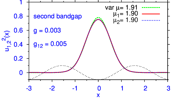
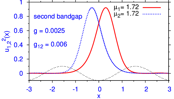
Figure 1: (Color online) Examples of unsplit and split symmetric solitons, with $N_{1}=N_{2}=1000$, trapped in potential $-V_{0}\cos(2x)$. Here and in all other figures, $V_{0}=5$. For the unsplit soliton, the variational profile is included too.

In all cases, the difference between the variational and numerical shapes of the unsplit solitons is extremely small. The present solitons are essentially confined to a single cell of the OL potential. They change the shape and develop undulating tails, which are often considered as a characteristic feature of GSs, when $\mu$ is taken very close to an edge of the bandgap (Fig. 1 demonstrates that, even in a well-pronounced split state, peaks of both components stay in a common cell). It is also observed that, as might be expected, the increase of the intra-species nonlinearity coefficient, $g$, pushes the solitons to higher bandgaps, while the increase of $g_{12}$ tends to split the two components of the soliton. In addition to the compact GSs presented here, there may also exist loosely bound ones, that extend over several OL EPL .

In Fig. 2, the entire family of the symmetric solitons is displayed in the parameter plane of the strength of the intra- and inter-species interactions, $\left(gN,g_{12}N\right)$. The VA prediction for border between the unsplit and split solitons, given by Eq. (11), provides a remarkably accurate fit to the numerical findings.

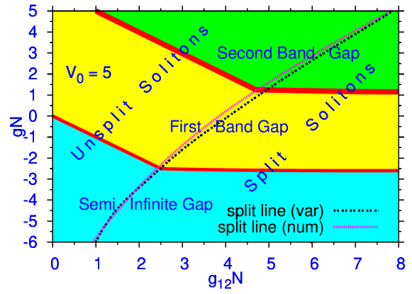
Figure 2: (Color online) The family of the two-component symmetric solitons ($N_{1}=N_{2}\equiv N$), mapped into the plane of the interaction strengths, $g_{12}N$ and $gN$. The plane is divided into regions corresponding to the semi-infinite gap and the finite first and second bandgaps. They are separated by narrow stripes representing the Bloch bands. The border between the unsplit and split solitons is shown as found from the numerical data, and as predicted by Eq. (11).

Dependences $N(\mu)$ for families of symmetric solitons are plotted in Fig. 3. It is known that a necessary stability condition for solitons populating the semi-infinite gap is given by the Vakhitov-Kolokolov (VK) criterion, $dN/d\mu<0$ VK , while stable solitons in finite bandgaps have $dN/d\mu>0$, disobeying this criterion GSprediction ; EPL . In the present case, Fig. 3 shows the same generic feature (the semi-infinite gap contains solitons only for $g<0$, i.e., in the case of the self-attraction). A noteworthy feature, viz., a turning point in dependence $N(\mu)$, is exhibited, for $g=-0.001$, by the solution branch which passes from the semi-infinite gap into the first finite bandgap, and also by the branch corresponding to $g=-0.0005$. Consequently, two different stable solitons can be found in the corresponding interval of $\mu$. The solitons belonging to the branches with $g=0.0025$, $g=0.001$ and $g=0$ in Fig. 3 are unsplit, and they are accurately predicted by the VA. Accordingly, the curves for these branches, as obtained from the VA and from the numerical data, are virtually identical. On the other hand, all solitons belonging to the branch with $g=-0.0025$ exhibit splitting. As concerns the bending branches, their parts below the turning point are formed by unsplit solitons (which are accurately approximated by the VA), while above the turning point the family continues in the split form. Accordingly, the turning point on each bending branch belongs to the splitting border for the symmetric solitons, cf. Fig. 2.

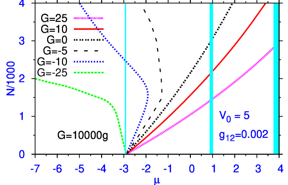
Figure 3: (Color online) The number of atoms in the symmetric soliton, $N_{1}=N_{2}\equiv N$, versus the common chemical potential of both components, at several values of $g$ for $g_{12}=0.002$. Vertical stripes are the Bloch bands between the gaps (the solution branch with $g=-0.001$ suffers a discontinuity when it hits the band separating the semi-infinite and first finite gaps).

Asymmetric solitons: Typical examples of solitons with $N_{1}\neq N_{2}$ are displayed in Fig. 4. Similar to their symmetric counterparts, cf. Fig. 1, they feature both unsplit and split shapes (the former ones are well approximated by the VA), which are again confined to a single cell of the OL potential.

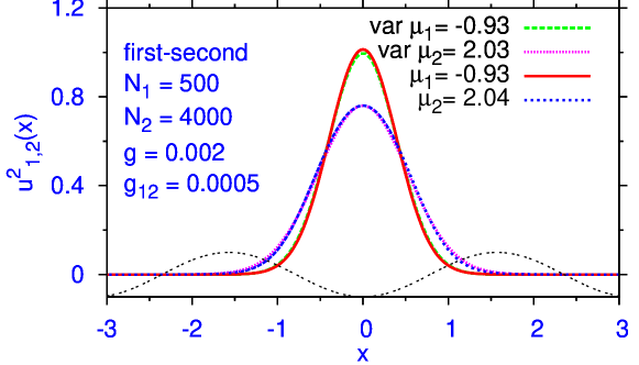
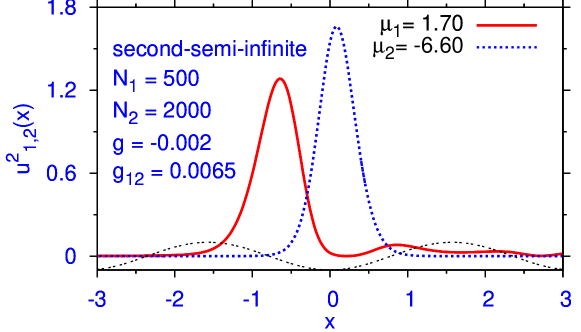
Figure 4: (Color online) Typical profiles of unsplit and split asymmetric ($N_{1}\neq N_{2}$) solitons. The examples represent solitons of inter-gap types, as indicated in the panels. For the unsplit soliton, the profiles predicted by the VA are shown too.

The entire family of asymmetric and symmetric GSs is mapped in the $\left(N_{1},N_{2}\right)$ plane, at fixed values of the interaction coefficients ($g_{12}$ and $g$), in Fig. 5. In these diagrams, the border between intra-gap solitons of different types shrink to a point belonging to the diagonal line ($N_{1}=N_{2}$), which corresponds to symmetric solitons that account for direct transitions between different types of intra-gap solitons. In Fig. 5 the VA for the unsplit solitons accurately predicts borders between their different varieties.

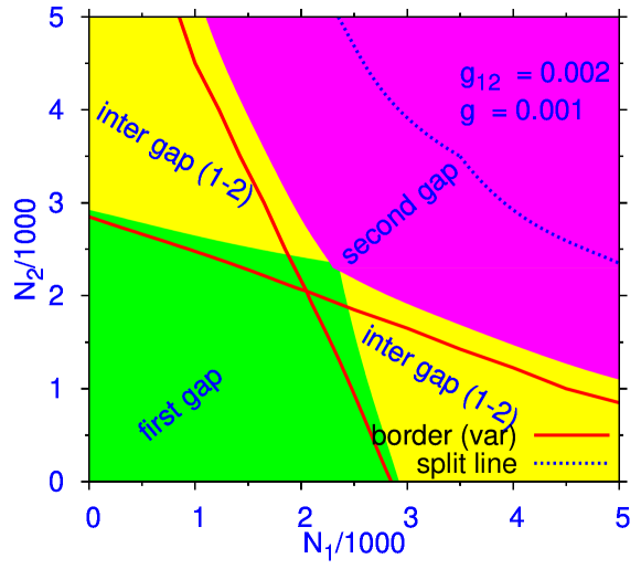
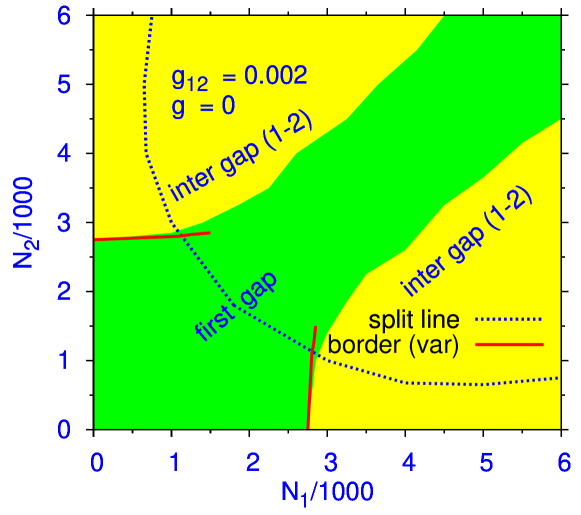
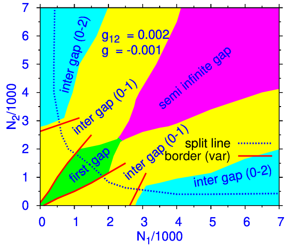
Figure 5: (Color online) Families of asymmetric and symmetric solitons mapped into the plane of atom numbers $N_{1}$ and $N_{2}$, for different $g_{12}$ and $g$. The plane is divided into regions populated by solitons of six different types (three intra-gap and three inter-gap varieties, symbols 0 and 1, 2 standing for the semi-infinite and two lowest finite bandgaps, respectively). Each panel also shows the numerically found border between the unsplit and split solitons, and borders between different types of the unsplit ones, as predicted by the VA.

If none of the nonlinearities is attractive [Figs. 5(a) and (b)], no chemical potential may fall in the semi-infinite gap. Three types of GSs are possible if both nonlinearities are repulsive [Fig. 5(a)]: intra-gap ones, in the two finite bandgaps, and the inter-gap species, combining them. If the intra-species nonlinearity exactly vanishes [Figs. 5(b)], the inter-species repulsion cannot push both components into the second finite bandgap, which leaves us with two species: intra-gap in the first bandgap, and the one mixing the two finite bandgaps. The interplay of the attractive intra-species nonlinearity with the inter-species repulsion supports two intra-gap and two inter-gap types, as seen in Fig. 5(c). Note that one of them skips the first bandgap, binding together components sitting in the semi-infinite and in second finite gaps. A notable feature of the map in Fig. 5(c) is the smooth transition from ordinary solitons, with both components in the semi-infinite gap, to ones of the semi-gap type.

IV Conclusion

In this work, we have considered the interplay of the repulsion between two species of bosonic atoms with intra-species repulsion or attraction in a binary BEC mixture loaded into the OL potential. Families of stable solitons found in this setting are classified as symmetric/asymmetric, split/unsplit, and intra/inter-gap. Three varieties of intra-gap solitons, and another three types of inter-gap ones are identified, if the consideration is limited to the two lowest finite bandgaps of the OL-induced spectrum. Varying the atom numbers in the two components, $N_{1,2}$, we have plotted maps of various states. Although different intra- and inter-gap species are separated by Bloch bands, transitions between them are continuous in the $\left(N_{1},N_{2}\right)$ plane. In particular, a solution branch which connects the solitons (of the split type), populating the semi-infinite gap, and unsplit solitons in the first finite bandgap, features the turning point at the border between the two varieties. Other varieties revealed by the analysis represent semi-gap solitons, with one component belonging to the semi-infinite gap, and the other one falling into a finite bandgap.

A considerable part of the numerical findings reported in this work was accurately predicted by variational approximation. These include the shape of unsplit solitons (both symmetric and asymmetric ones), borders between their varieties, and the splitting border for the symmetric solitons.

We appreciate support from FAPESP and CNPq (Brazil), and Israel Science Foundation (Center-of-Excellence grant No. 8006/03).

References

- (1) V. M. Pérez-García, H. Michinel, and H. Herrero, Phys. Rev. A 57, 3837 (1998); F. Kh. Abdullaev et al., Int. J. Mod. Phys. B 19, 3415 (2005).
- (2) K. E. Strecker et al., Nature 417, 150 (2002); L. Khaykovich et al., Science 256, 1290 (2002); S. L. Cornish, S. T. Thompson and C. E. Wieman, Phys. Rev. Lett. 96, 170401 (2006).
- (3) O. Zobay et al., Phys. Rev. A 59, 643 (1999); A. Trombettoni and A. Smerzi, Phys. Rev. Lett. 86, 2353 (2001); B. B. Baizakov, V. V. Konotop, and M. Salerno, J. Phys. B 35, 51015 (2002); P. J. Y. Louis et al., Phys. Rev. A 67, 013602 (2003).
- (4) K. M. Hilligsøe, M. K. Oberthaler, and K.-P. Marzlin, Phys. Rev. A 66, 063605 (2002); D. E. Pelinovsky, A. A. Sukhorukov and Y. S. Kivshar, Phys. Rev. E 70, 036618 (2004).
- (5) B. Eiermann et al., Phys. Rev. Lett. 92, 230401 (2004); O. Morsch and M. Oberthaler, Rev. Mod. Phys. 78, 179 (2006).
- (6) V. Ahufinger et al., Phys. Rev. A 69, 053604 (2004).
- (7) M. Matuszewski et al., Phys. Rev. A 73, 063621 (2006).
- (8) C. J. Myatt et al.,Phys. Rev. Lett. 78, 586 (1997); D. M. Stamper-Kurn et al., Phys. Rev. Lett. 80, 2027 (1998).
- (9) A. Simoni et al. , Phys. Rev. Lett. 90, 163202 (2003).
- (10) V. M. Pérez-García and J. B. Beitia, Phys. Rev. A 72, 033620 (2005); S. K. Adhikari, Phys. Lett. A 346, 179 (2005); Phys. Rev. A 72, 053608 (2005); J. Phys. A 40, 2673 (2007).
- (11) A. Gubeskys, B. A. Malomed, and I. M. Merhasin, Phys. Rev. A 73, 023607 (2006).
- (12) M. Matuszewski, B. A. Malomed, and M. Trippenbach, Phys. Rev. A. 76, 043826 (2007).
- (13) V. M. Pérez-García et al., Phys. Rev. A 56 1424 (1997).
- (14) L. Salasnich, A. Parola, and L. Reatto, Phys. Rev. A 65, 043614 (2002); L. Salasnich and B. A. Malomed, Phys. Rev. A 74, 053610 (2006).
- (15) S. K. Adhikari and B. A. Malomed, Europhys. Lett. 79, 50003 (2007); Phys. Rev. A 76, 043626 (2007).
- (16) M. G. Vakhitov and A. A. Kolokolov, Izv. Vuz. Radiofiz. 16, 1020 (1973) [Sov. J. Radiophys. Quantum Electr. 16, 783 (1973)].