Dynamics of Annihilation I : Linearized Boltzmann Equation and Hydrodynamics

Abstract

We study the non-equilibrium statistical mechanics of a system of freely moving particles, in which binary encounters lead either to an elastic collision or to the disappearance of the pair. Such a system of ballistic annihilation therefore constantly looses particles. The dynamics of perturbations around the free decay regime is investigated from the spectral properties of the linearized Boltzmann operator, that characterize linear excitations on all time scales. The linearized Boltzmann equation is solved in the hydrodynamic limit by a projection technique, which yields the evolution equations for the relevant coarse-grained fields and expressions for the transport coefficients. We finally present the results of Molecular Dynamics simulations that validate the theoretical predictions.

I Introduction

Understanding the differences and similarities between a flow of macroscopic grains and that of an ordinary liquid is an active field of research g05 ; d07b . From a fundamental perspective, it is tempting to draw a correspondence between the grains of the former and the atoms of the latter in order to make use of the powerful tools of statistical mechanics to derive a large scale description for the various fields of interest, such as the local density of grains. A key difference between a granular system and an ordinary liquid is that collisions between macroscopic grains dissipate energy, due to the redistribution of translational kinetic energy into internal modes. This simple fact has far reaching consequences bte05 ; d07b , but also poses an a priori serious problem concerning the validity of the procedure leading to the hydrodynamic description. Indeed, the standard approach retains in the coarse-grained description only those fields associated with quantities that are conserved in collisions (such as density and momentum). There is however good evidence –both numerical and theoretical– that in the granular case, a relevant description should include the kinetic temperature field, defined as the kinetic energy density (bclibro2001 ; d07b and references therein), which is therefore not associated to a conserved quantity.

Our purpose here is to test a hydrodynamic description with suitable coarse-grained fields, for a model system where not only the kinetic energy is not conserved during binary encounters, but also the number of particles and the linear momentum. The ballistic annihilation model bnklr ; bek ; ks ; t02 ; ptd02 ; llf06 provides a valuable candidate: in this model, each particle moves freely (ballistically) until it meets another particle; such binary encounters lead to the annihilation of the colliding pair of particles. In addition, we introduce a parameter $0\leq p\leq 1$ that may be thought of as a measure of the distance to equilibrium, so that an ensemble of spherical particles in dimension $d$ undergoing ballistic motion either annihilate upon contact (with probability $p$) or scatter elastically (with probability $1-p$). For the corresponding probabilistic ballistic annihilation model, the Chapman-Enskog chapman60 scheme was applied recently cdt04 . The hydrodynamic equations were derived and explicit formulas for the transport coefficients obtained. Our goal here is two-fold. First, we would like to shed light on the context and limitations of the derivation, by obtaining the hydrodynamic description directly from the linearized Boltzmann equation. Second, we aim at putting to the test the theoretical framework thereby obtained by careful comparison with numerical simulations of the annihilation process. For granular gas dynamics, the same program is quite complete, although challenges remain g05 ; d07b . The objective here is to initiate a similar formulation for the ballistic annihilation model in view of a more stringent test of the hydrodynamic machinery.

The paper is organized as follows. We start in section II with a reminder of results derived in Refs t02 ; ptd02 . The kinetic description adopted is that of the Boltzmann equation, since it has been shown that for $p=1$ (all collision events leading to annihilation), the underlying molecular chaos closure provides an exact description at long times, provided space dimension $d$ is strictly larger than $1$ ptd02 . We may assume that the same holds for an arbitrary but non vanishing value of $p$, since the density is then still a decreasing function of time. The focus is here on an unforced system, which is characterized by an algebraic decay with time of the total density and kinetic energy density (homogeneous decay state) t02 ; ptd02 . More precisely, we are interested in small perturbations around this state, so that the Boltzmann equation will be subsequently linearized. After having identified the operator that generates the dynamics of fluctuations, attention will be paid in section III to its spectral properties. This will provide the basis for finding in section IV the evolution equations for the hydrodynamic fields (i.e. those chosen for the coarse-grained description) and for obtaining explicit formulas for the transport coefficients. Finally, our predictions will be confronted in section V against extensive Molecular Dynamics simulations. Such a comparison is an essential step in testing the foundations of the hydrodynamic treatment.

II The Boltzmann Equation approach to the Homogeneous Decay State

II.1 Non-linear description

The Boltzmann equation describes the time evolution of the one particle distribution function $f(\mathbf{r},\mathbf{v}_{1},t)$. For a system of smooth hard disks or spheres of mass $m$ and diameter $\sigma$, which annihilate with probability $p$ or collide elastically with probability $1-p$, it has the form

$$\left(\frac{\partial}{\partial t}+\mathbf{v}_{1}\cdot\nabla\right)f(\mathbf{r},\mathbf{v}_{1},t)=pJ_{a}[f|f]+(1-p)J_{c}[f|f],$$ (1)

where the annihilation operator $J_{a}$ is defined by ptd02

$$J_{a}[f|g]=-\sigma^{d-1}\int\!\!d\mathbf{v}_{2}\!\!\int\!\!d\hat{\bm{\sigma}}\Theta(\mathbf{v}_{12}\cdot\hat{\bm{\sigma}})(\mathbf{v}_{12}\cdot\hat{\bm{\sigma}})f(\mathbf{r},\mathbf{v}_{1},t)g(\mathbf{r},\mathbf{v}_{2},t).$$ (2)

The elastic collision operator $J_{c}$ reads br04 ; l81

$$J_{c}[f|g]=\sigma^{d-1}\int\!\!d\mathbf{v}_{2}\!\!\int\!\!d\hat{\bm{\sigma}}\Theta(\mathbf{v}_{12}\cdot\hat{\bm{\sigma}})(\mathbf{v}_{12}\cdot\hat{\bm{\sigma}})(b_{\sigma}^{-1}-1)f(\mathbf{r},\mathbf{v}_{1},t)g(\mathbf{r},\mathbf{v}_{2},t),$$ (3)

with $\mathbf{v}_{12}=\mathbf{v}_{1}-\mathbf{v}_{2}$, $\Theta$ the Heaviside step function, $\hat{\bm{\sigma}}$ a unit vector joining the centers of the two particles at contact and $b_{\sigma}^{-1}$ an operator replacing all the velocities $\mathbf{v}_{1}$ and $\mathbf{v}_{2}$ appearing in its argument by their precollisional values $\mathbf{v}_{1}^{*}$ and $\mathbf{v}_{2}^{*}$, given by

$$b_{\sigma}^{-1}\mathbf{v}_{1}=\mathbf{v}_{1}^{*} = \mathbf{v}_{1}-(\mathbf{v}_{12}\cdot\hat{\bm{\sigma}})\hat{\bm{\sigma}},$$ (4)

$$b_{\sigma}^{-1}\mathbf{v}_{2}=\mathbf{v}_{2}^{*} = \mathbf{v}_{2}+(\mathbf{v}_{12}\cdot\hat{\bm{\sigma}})\hat{\bm{\sigma}}.$$ (5)

We assume that the system can be characterized macroscopically by coarse grained (hydrodynamic-like) fields, that we define as in standard Kinetic Theory in terms of the local velocity distribution function $f(\mathbf{r},\mathbf{v},t)$

$$n(\mathbf{r},t) = \int\!d\mathbf{v}f(\mathbf{r},\mathbf{v},t),$$ (6)

$$n(\mathbf{r},t)\mathbf{u}(\mathbf{r},t) = \int\!d\mathbf{v}\mathbf{v}f(\mathbf{r},\mathbf{v},t),$$ (7)

$$\frac{d}{2}n(\mathbf{r},t)T(\mathbf{r},t) = \int\!d\mathbf{v}\frac{m}{2}V^{2}f(\mathbf{r},\mathbf{v},t),$$ (8)

where $n(\mathbf{r},t)$, $\mathbf{u}(\mathbf{r},t)$, and $T(\mathbf{r},t)$ are the local number density, velocity, and temperature, respectively. We have introduced here $\mathbf{V}=\mathbf{v}-\mathbf{u}$, the velocity of the particle relative to the local velocity flow. We stress that the temperature defined has a kinetic meaning only, but lacks a thermodynamic interpretation. It seems natural to consider these fields, as they are the usual hydrodynamical fields of the equilibrium system (with $p=0$). It is however not obvious at this point that restricting our coarse-grained description to the above three fields provides a relevant and consistent framework. A major goal of this paper is to provide strong hints that this is indeed the case. We will show in particular that closed equations can be obtained for these fields in the appropriate time and length scales, under reasonable assumptions.

The Boltzmann equation (1) admits a homogeneous scaling solution $f_{H}$ in which all the time dependence is embedded in the hydrodynamic fields, with the further simplification that those fields are position independent. The existence of this regime could not be shown rigorously, but, numerically, such a scaling solution quickly emerges from an arbitrary initial condition t02 ; ptd02 . It has the form ptd02

$$f_{H}(\mathbf{v},t)=\frac{n_{H}(t)}{v_{H}(t)^{d}}\chi_{H}(\mathbf{c}),\qquad\hbox{with }\mathbf{c}=\frac{\mathbf{v}}{v_{H}(t)},$$ (9)

where

$$v_{H}(t)=\left[\frac{2T_{H}(t)}{m}\right]^{1/2}$$ (10)

is the “thermal” (root-mean-square) velocity and $\chi_{H}(\mathbf{c})$ is an isotropic function depending only on the modulus $c=|\mathbf{c}|$ of the rescaled velocity. By taking moments in the Boltzmann equation and using the scaling (9), it can be seen that the homogeneous density and temperature obey the equations cdt04

$$\frac{\partial n_{H}(t)}{\partial t} = -p\nu_{H}(t)\zeta_{n}n_{H}(t),$$ (11)

$$\frac{\partial T_{H}(t)}{\partial t} = -p\nu_{H}(t)\zeta_{T}T_{H}(t),$$ (12)

where we have introduced the collision frequency of the corresponding hard sphere fluid in equilibrium (with same temperature and density)

$$\nu_{H}(t)=\frac{n_{H}(t)\,T^{1/2}_{H}(t)\,\sigma^{d-1}}{m^{1/2}}\frac{8\pi^{\frac{d-1}{2}}}{(d+2)\Gamma(d/2)}$$ (13)

and the dimensionless decay rates $\zeta_{n}$ and $\zeta_{T}$, that are functionals of the distribution function

$$p\zeta_{n} = -\frac{\gamma}{2}\int\!\!d\mathbf{c}_{1}\!\!\int\!\!d\mathbf{c}_{2}T(\mathbf{c}_{1},\mathbf{c}_{2})\chi_{H}(\mathbf{c}_{1})\chi_{H}(\mathbf{c}_{2}),$$ (14)

$$p\zeta_{T} = -\frac{\gamma}{2}\int\!\!d\mathbf{c}_{1}\!\!\int\!\!d\mathbf{c}_{2}\left(\frac{2c_{1}^{2}}{d}-1\right)T(\mathbf{c}_{1},\mathbf{c}_{2})\chi_{H}(\mathbf{c}_{1})\chi_{H}(\mathbf{c}_{2}).$$ (15)

In these expressions, $\gamma$ is a quantity that does not depend on time, which reads

$$\gamma=\frac{2n_{H}(t)v_{H}(t)\sigma^{d-1}}{\nu_{H}(t)}=\frac{(d+2)\sqrt{2}\Gamma(d/2)}{4\pi^{(d-1)/2}},$$ (16)

and the binary collision operator $T(\mathbf{c}_{1},\mathbf{c}_{2})$, that should not be confused with the temperature, takes the form

$$T(\mathbf{c}_{1},\mathbf{c}_{2})=\int\!\!d\hat{\bm{\sigma}}\Theta(\mathbf{c}_{12}\cdot\hat{\bm{\sigma}})(\mathbf{c}_{12}\cdot\hat{\bm{\sigma}})[(1-p)b_{\sigma}^{-1}-1].$$ (17)

Finally, we can write an equation for the scaled distribution function $\chi_{H}(\mathbf{c})$ in terms of the coefficients and operators defined above

$$p\left[(d\zeta_{T}-2\zeta_{n})+\zeta_{T}\mathbf{c}_{1}\cdot\frac{\partial}{\partial\mathbf{c}_{1}}\right]\chi_{H}(\mathbf{c}_{1})=\gamma\int\!\!d\mathbf{c}_{2}T(\mathbf{c}_{1},\mathbf{c}_{2})\chi_{H}(\mathbf{c}_{1})\chi_{H}(\mathbf{c}_{2}).$$ (18)

The operator $b_{\sigma}^{-1}$ in the last equation is defined again by equation (4), but substituting $(\mathbf{v}_{1},\mathbf{v}_{2})$ by $(\mathbf{c}_{1},\mathbf{c}_{2})$.

Although an exact and explicit solution of equation (18) is not known, its behavior at large and small velocities has been determined t02 ; ptd02 . In this work we will use the approximate form of the distribution function in the so-called first Sonine approximation (an expansion around a Gaussian functional form, see Appendix A), which is valid for velocities in the thermal region, and all the functionals of $\chi_{H}(\mathbf{c})$, that is the decay rates and the transport coefficients, will be evaluated in this approximation cdt04s ; t02 .

II.2 Linearized Boltzmann Equation

In the remainder, we consider a situation where the system is very close to the homogeneous decay state, so that we can write

$$f(\mathbf{r},\mathbf{v}_{1},t)=f_{H}(\mathbf{v}_{1},t)+\delta f(\mathbf{r},\mathbf{v}_{1},t),\qquad|\delta f(\mathbf{r},\mathbf{v}_{1},t)|\ll f_{H}(\mathbf{v}_{1},t).$$ (19)

Substitution of equation (19) into the Boltzmann equation (1), keeping only linear terms in $\delta f$, yields

$$\left(\frac{\partial}{\partial t}+\mathbf{v}_{1}\cdot\nabla\right)\delta f(\mathbf{r},\mathbf{v}_{1},t)$$

$$=p\left\{J_{a}[\delta f|f_{H}]+J_{a}[f_{H}|\delta f]\right\}+(1-p)\left\{J_{c}[\delta f|f_{H}]+J_{c}[f_{H}|\delta f]\right\},$$ (20)

Given the scaling form of $f$ (Eq. (9)), it is convenient to introduce as well the scaled deviation of the distribution function, $\delta\chi$, as follows

$$\delta f(\mathbf{r},\mathbf{v}_{1},t)=\frac{n_{H}(t)}{v_{H}(t)^{d}}\delta\chi(\mathbf{r},\mathbf{c}_{1},\tau)\ .$$ (21)

Moreover, Eqs. (11) and (12) suggest to use the dimensionless time scale $\tau$ defined by

$$\tau=\frac{1}{2}\int_{0}^{t}dt^{\prime}\nu_{H}(t^{\prime}),$$ (22)

which counts the number of collision per particle in the time interval $[0,t]$. Combining Eq. (13) together with Eq. (11, 12) yields immediately $\nu_{H}(t)=(1/\nu_{H}(0)+p(\zeta_{n}+\zeta_{T}/2)t)^{-1}$ and thus

$$\tau=\frac{1}{p(2\zeta_{n}+\zeta_{T})}\log[1+\nu_{H}(0)p(\zeta_{n}+\zeta_{T}/2)t]\;.$$ (23)

In this time scale $\tau$ (22), these equations (11, 12) are easily integrated, yielding

$$n_{H}(\tau)=n_{H}(0)\exp(-2p\zeta_{n}\tau),\qquad T_{H}(\tau)=T_{H}(0)\exp(-2p\zeta_{T}\tau),$$ (24)

and power law behaviors in time $t$, $n_{H}(t)\propto t^{-2\zeta_{n}/(2\zeta_{n}+\zeta_{T})}$ and $T_{H}(t)\propto t^{-2\zeta_{T}/(2\zeta_{n}+\zeta_{T})}$ at large time $t\gg 1$ . It proves also convenient to introduce Fourier components [with the notation ${h}_{\mathbf{k}}=\int\!\!d\mathbf{r}\exp^{-i\mathbf{k}\cdot\mathbf{r}}h(\mathbf{r})$] so that the evolution equation for a general $\mathbf{k}$ component of $\delta\chi$ is, in the $\tau$ timescale,

$$\frac{\partial}{\partial\tau}\delta{\chi}_{\mathbf{k}}(\mathbf{c}_{1},\tau)=\left[\Lambda(\mathbf{c}_{1})-il_{H}(\tau)\mathbf{k}\cdot\mathbf{c}_{1}\right]\delta{\chi}_{\mathbf{k}}(\mathbf{c}_{1},\tau).$$ (25)

In this equation, the time dependent length scale $l_{H}=2v_{H}(\tau)/\nu_{H}(\tau)$ is proportional to the instantaneous mean free path ($l_{H}(\tau)\propto n_{H}^{-1}(\tau)$, see Eq. (13)) and the homogeneous scaled Boltzmann linear operator reads

$$\Lambda(\mathbf{c}_{1})h(\mathbf{c}_{1})=\gamma\int\!\!d\mathbf{c}_{2}T(\mathbf{c}_{1},\mathbf{c}_{2})(1+{\cal P}_{12})\chi_{H}(\mathbf{c}_{1})h(\mathbf{c}_{2})$$

$$+p(2\zeta_{n}-d\zeta_{T})h(\mathbf{c}_{1})-p\zeta_{T}\mathbf{c}_{1}\cdot\frac{\partial}{\partial\mathbf{c}_{1}}h(\mathbf{c}_{1}).$$ (26)

In this expression, the permutation operator ${\cal P}_{12}$ interchanges the labels of particles $1$ and $2$ and subsequently allows for more compact notations. In the present representation, all the time dependence due to the reference state is absorbed in the mean free path, obtained from $l_{H}(\tau)\propto n_{H}^{-1}(\tau)$ as

$$l_{H}(\tau)=l_{H}(0)\exp(2p\zeta_{n}\tau),$$ (27)

which, as expected, is an increasing function of time.

II.3 Linearized Hydrodynamic Equations around the homogeneous decay state

Let us define the relative deviations of the hydrodynamic fields from their homogeneous values by

$$\rho(\mathbf{r},\tau)\equiv\frac{\delta n(\mathbf{r},\tau)}{n_{H}(\tau)} = \int\!\!d\mathbf{c}\delta\chi(\mathbf{r},\mathbf{c},\tau),$$ (28)

$$\mathbf{w}(\mathbf{r},\tau)\equiv\frac{\delta\mathbf{u}(\mathbf{r},\tau)}{v_{H}(\tau)} = \int\!\!d\mathbf{c}\mathbf{c}\delta\chi(\mathbf{r},\mathbf{c},\tau),$$ (29)

$$\theta(\mathbf{r},\tau)\equiv\frac{\delta T(\mathbf{r},\tau)}{T_{H}(\tau)} = \int\!\!d\mathbf{c}\left(\frac{2c^{2}}{d}-1\right)\delta\chi(\mathbf{r},\mathbf{c},\tau),$$ (30)

where $\delta y(\mathbf{r},\tau)\equiv y(\mathbf{r},\tau)-y_{H}(t)$ denotes the deviation of a local macroscopic variable, $y(\mathbf{r},\tau)$, from its homogeneous decay state value, $y_{H}(t)$. Taking velocity moments in the Boltzmann equation (25), we obtain the linearized balance equation for the $\mathbf{k}$ components of the hydrodynamic fields

$$\left(\frac{\partial}{\partial\tau}-2p\zeta_{n}\right){\rho}_{\mathbf{k}}+il_{H}(\tau)\mathbf{k}\cdot{\mathbf{w}}_{\mathbf{k}}-p\ \delta\zeta_{n}[\delta\chi_{\mathbf{k}}]=0,$$ (31)

$$\left[\frac{\partial}{\partial\tau}-p(2\zeta_{n}+\zeta_{T})\right]{\mathbf{w}}_{\mathbf{k}}$$

$$\qquad+\frac{i}{2}l_{H}(\tau)\mathbf{k}({\rho}_{\mathbf{k}}+{\theta}_{\mathbf{k}})+il_{H}(\tau)\mathbf{k}\cdot\bm{\Pi}[\delta\chi_{\mathbf{k}}]-p\ \delta\bm{\zeta}_{u}[\delta\chi_{\mathbf{k}}]=0,$$ (32)

$$\left[\frac{\partial}{\partial\tau}-2p(\zeta_{n}+\zeta_{T})\right]{\theta}_{\mathbf{k}}$$

$$\qquad-2p\zeta_{T}{\rho}_{\mathbf{k}}+i\frac{2}{d}l_{H}(\tau)\mathbf{k}\cdot({\mathbf{w}}_{\mathbf{k}}+\bm{\phi}[\delta\chi_{\mathbf{k}}])-p\ \delta\zeta_{T}[\delta\chi_{\mathbf{k}}]=0.$$ (33)

Here, we have introduced the traceless pressure tensor and the heat flux as

$$\bm{\Pi}[\delta\chi_{\mathbf{k}}] = \int\!\!d\mathbf{c}\bm{\Delta}(\mathbf{c})\delta{\chi}_{\mathbf{k}}(\mathbf{c},\tau),$$ (34)

$$\bm{\phi}[\delta\chi_{\mathbf{k}}] = \int\!\!d\mathbf{c}\bm{\Sigma}(\mathbf{c})\delta{\chi}_{\mathbf{k}}(\mathbf{c},\tau),$$ (35)

where $\bm{\Delta}$ and $\bm{\Sigma}$ are defined as

$$\Delta_{ij}(\mathbf{c}) = c_{i}c_{j}-\frac{c^{2}}{d}\delta_{ij},$$ (36)

$$\bm{\Sigma}(\mathbf{c}) = \left(c^{2}-\frac{d+2}{2}\right)\mathbf{c},$$ (37)

and the functionals

$$p\ \delta\zeta_{n}[\delta\chi]=\gamma\int\!\!d\mathbf{c}_{1}\!\!\int\!\!d\mathbf{c}_{2}T(\mathbf{c}_{1},\mathbf{c}_{2})(1+{\cal P}_{12})\chi_{H}(\mathbf{c}_{1})\delta{\chi}_{\mathbf{k}}(\mathbf{c}_{2},\tau),$$ (38)

$$p\ \delta\bm{\zeta}_{u}[\delta\chi]=\gamma\int\!\!d\mathbf{c}_{1}\!\!\int\!\!d\mathbf{c}_{2}\mathbf{c}_{1}T(\mathbf{c}_{1},\mathbf{c}_{2})(1+{\cal P}_{12})\chi_{H}(\mathbf{c}_{1})\delta{\chi}_{\mathbf{k}}(\mathbf{c}_{2},\tau),$$ (39)

$$p\ \delta\zeta_{T}[\delta\chi]=\gamma\int\!\!d\mathbf{c}_{1}\!\!\int\!\!d\mathbf{c}_{2}\left(\frac{2c_{1}^{2}}{d}-1\right)T(\mathbf{c}_{1},\mathbf{c}_{2})(1+{\cal P}_{12})\chi_{H}(\mathbf{c}_{1})\delta{\chi}_{\mathbf{k}}(\mathbf{c}_{2},\tau).$$ (40)

The previous analysis therefore amounts to obtaining a set of complicated equations expressing the evolution of the hydrodynamic fields as a function of the rescaled homogeneous distribution function $\chi_{H}$ and the perturbation $\delta{\chi}$. In order to obtain a closed set of equations for the hydrodynamic fields (31), (II.3), (II.3), we need therefore to express the functionals $\bm{\Pi}$, $\bm{\phi}$, $\delta\zeta_{n}$, $\delta\bm{\zeta}_{u}$ and $\delta\zeta_{T}$, in terms of the hydrodynamic fields themselves. We will see in the next section that, as long as we can treat $l_{H}(\tau)\mathbf{k}$ as a small parameter and if the linear Boltzmann operator has some specific properties, it is possible to carry out this program and to close the linear hydrodynamic equations. However, since the mean free path $l_{H}(\tau)$ increases with time (Eq. (27)), the requirement of a small $l_{H}(\tau)\mathbf{k}$ is necessarily limited to a time window depending on both $\mathbf{k}$ and the probability of annihilation $p$. An upper bound for this window is provided by the time when the mean free path becomes of the order of the system size.

III Solution of the Linearized Boltzmann Equation

In this Section we explore the solutions to the linearized Boltzmann equation (25) and establish some properties of the homogeneous linear Boltzmann operator that will be essential for the coarse-grained description. From the expression of the linearized Boltzmann equation, we can identify the operator $\Lambda-i\mathbf{k}\cdot\mathbf{c}l_{H}(\tau)$ as the “generator of the dynamic” of $\delta\chi_{\mathbf{k}}$. As we are interested in the solutions of this equation in the hydrodynamic regime (large enough scales), it is convenient to study first the eigenvalue problem of the homogeneous linear Boltzmann operator. The inhomogeneous term will be treated perturbatively later on.

III.1 Hydrodynamic Eigenfunctions of $\Lambda$

Let us consider the eigenvalue problem of the homogeneous linear Boltzmann operator $\Lambda$

$$\Lambda(\mathbf{c})\xi_{\beta}(\mathbf{c})=\lambda_{\beta}\xi_{\beta}(\mathbf{c}).$$ (41)

Finding all the solutions of this equation is an insurmountable task. Nevertheless, it is possible to obtain some particular solutions, which will turn out to be the relevant ones in the hydrodynamic regime. The problem will be posed in a Hilbert space of functions of $\mathbf{c}$ with scalar product given by

$$\langle g|h\rangle=\int\!\!d\mathbf{c}\chi_{H}^{-1}(\mathbf{c})g^{*}(\mathbf{c})h(\mathbf{c}),$$ (42)

where $g^{*}$ denotes the complex conjugate of $g$.

Of particular interest here are the eigenfunctions and eigenvalues associated with linear hydrodynamics. Following bdrlibro2003 ; bd05 , we use the fact that the homogeneous decay state is parameterized by the hydrodynamic fields $n_{H}$, $T_{H}$ and $\mathbf{u}_{H}$. Writing the Boltzmann equation satisfied by $\chi_{H}$ and differentiating it with respect to these fields allows then to obtain three exact relations from which one can extract eigenfunctions of the linearized Boltzmann collision operator. In Appendix B, we show that the functions

$$\xi_{1}(\mathbf{c}) = \chi_{H}(\mathbf{c})+\frac{\partial}{\partial\mathbf{c}}\cdot\left[\mathbf{c}\chi_{H}(\mathbf{c})\right],$$ (43)

$$\xi_{2}(\mathbf{c}) = z\chi_{H}(\mathbf{c})-\frac{\partial}{\partial\mathbf{c}}\cdot\left[\mathbf{c}\chi_{H}(\mathbf{c})\right],$$ (44)

$$\bm{\xi}_{3}(\mathbf{c}) = -\frac{\partial}{\partial\mathbf{c}}\chi_{H}(\mathbf{c}),$$ (45)

with $z=2\zeta_{n}/\zeta_{T}$, are solutions of Eq. (41), with eigenvalues

$$\lambda_{1}=0,\qquad\lambda_{2}=-p(\zeta_{T}+2\zeta_{n}),\qquad\lambda_{3}=p\zeta_{T},$$ (46)

respectively, $\lambda_{3}$ being $d$-fold degenerate. Although we cannot prove in general that these eigenvalues are indeed the hydrodynamic ones (i.e the upper part of the spectrum), we will assume that this is the case ; the self-consistency of the approach and comparison with numerical simulations will validate this assumption. Interestingly, in the particular case of Maxwell molecules where the full spectrum of $\Lambda$ may be computed exactly (see Appendix C), it appears that the above “hydrodynamic” modes dominate at long times, provided that $p<1/4$. For larger values of $p$, the “kinetic” mode with largest eigenvalue decays slower than one of the three “hydrodynamic” modes.

As a consequence of the non-hermitian character of the operator $\Lambda$, the functions $\{\xi_{\beta}\}_{\beta=1,\ldots,3}$ are not orthogonal with respect to the scalar product defined in (42). They are nevertheless independent and, in order to define the projection onto the subspace spanned by these functions, it is necessary to introduce a set of functions $\{\bar{\xi}_{\beta}\}_{\beta=1,\ldots,3}$ verifying the biorthonormality condition

$$\langle\bar{\xi}_{\beta}|\xi_{\beta^{\prime}}\rangle=\delta_{\beta,\beta^{\prime}}.$$ (47)

Although the set $\{\bar{\xi}_{\beta}\}_{\beta=1,\ldots,3}$ is not unique, a convenient choice is given by

$$\bar{\xi}_{1}(\mathbf{c}) = \left[\frac{2+z}{2(1+z)}-\frac{z}{1+z}\frac{c^{2}}{d}\right]\chi_{H}(\mathbf{c}),$$ (48)

$$\bar{\xi}_{2}(\mathbf{c}) = \left[\frac{1}{2(1+z)}+\frac{1}{1+z}\frac{c^{2}}{d}\right]\chi_{H}(\mathbf{c}),$$ (49)

$$\bar{\bm{\xi}}_{3}(\mathbf{c}) = \mathbf{c}\chi_{H}(\mathbf{c}).$$ (50)

Indeed, the functions $\{\bar{\xi}_{\beta}\}_{\beta=1,\ldots,3}$ have to be linear combinations of $\chi_{H}(c)$, $\mathbf{c}\chi_{H}(c)$ and $c^{2}\chi_{H}(c)$ to ensure that projection of $\delta\chi_{\mathbf{k}}$ onto the $\{\bar{\xi}_{\beta}\}$ yields the coarse-grained fields $\rho_{\mathbf{k}}$, $\theta_{\mathbf{k}}$ and $\mathbf{w}_{\mathbf{k}}$, or combinations thereof. The functions $\{\bar{\xi}_{\beta}\}_{\beta=1,\ldots,3}$ span a dual subspace of that spanned by the eigenfunctions and for any linear combination of the hydrodynamic modes

$$g(\mathbf{c})=\sum_{\beta=1}^{3}a_{\beta}\xi_{\beta}(\mathbf{c}),$$ (51)

the coefficients $a_{\beta}$ are given by

$$a_{\beta}=\langle\bar{\xi}_{\beta}|g\rangle=\int\!\!d\mathbf{c}\chi_{H}^{-1}(\mathbf{c})\bar{\xi}_{\beta}(\mathbf{c})g(\mathbf{c}).$$ (52)

In particular, the projection of the distribution function $\delta\chi_{\mathbf{k}}$ on the subspace spanned by the functions $\xi_{\beta}$ is given by the coefficients

$$\{\langle\bar{\xi}_{\beta}|\delta\chi_{\mathbf{k}}\rangle\}=\left\{\frac{1}{1+z}\rho_{\mathbf{k}}-\frac{z}{2(1+z)}\theta_{\mathbf{k}},\frac{1}{1+z}\rho_{\mathbf{k}}+\frac{1}{2(1+z)}\theta_{\mathbf{k}},\mathbf{w}_{\mathbf{k}}\right\}.$$ (53)

Notably, these coefficients are simply linear combinations of the hydrodynamic fields linearized around the homogeneous decay state.

III.2 Projection of the Linearized Boltzmann Equation on the Hydrodynamic Subspace

In this section, we study the linearized Boltzmann equation on the hydrodynamic subspace. Let us define the projectors

$$Ph(\mathbf{c})=\sum_{\beta=1}^{3}\langle\bar{\xi}_{\beta}|h\rangle\xi_{\beta}(\mathbf{c}),$$ (54)

and

$$P_{\perp}=1-P.$$ (55)

so that any function can be decomposed as

$$h(\mathbf{c})=Ph(\mathbf{c})+P_{\perp}h(\mathbf{c}).$$ (56)

In the definition (54) we are considering the functions (43)-(45) and (48)-(50) defined above.

Let us now consider the function $\delta\chi_{\mathbf{k}}$. If we apply the projectors $P$ and $P_{\perp}$ to equation (25), we obtain the following relations

$$\left[\frac{\partial}{\partial\tau}-P(\Lambda-il_{H}\mathbf{k}\cdot\mathbf{c})P\right]P\delta\chi_{\mathbf{k}}=-Pil_{H}\mathbf{k}\cdot\mathbf{c}P_{\perp}\delta\chi_{\mathbf{k}}+P\Lambda P_{\perp}\delta\chi_{\mathbf{k}},$$ (57)

$$\left[\frac{\partial}{\partial\tau}-P_{\perp}(\Lambda-il_{H}\mathbf{k}\cdot\mathbf{c})P_{\perp}\right]P_{\perp}\delta\chi_{\mathbf{k}}=-P_{\perp}il_{H}\mathbf{k}\cdot\mathbf{c}P\delta\chi_{\mathbf{k}},$$ (58)

where we have used that

$$P_{\perp}\Lambda P=0\ ,$$ (59)

which is obtained straightforwardly since $\xi_{\beta}$ are right-eigenfunctions of $\Lambda$. We note however that the $\{\bar{\xi}_{\beta}\}_{\beta=1,\ldots,3}$ are not left-eigenfunctions of $\Lambda$, so that $P\Lambda P_{\perp}\neq 0$. This also means that $P$ and $\Lambda$ do not commute.

Equations (57) and (58) for the functions $P\delta\chi_{\mathbf{k}}$ and $P_{\perp}\delta\chi_{\mathbf{k}}$ are coupled. Nevertheless, we shall see that, under certain conditions, we can decouple the equation for $P\delta\chi_{\mathbf{k}}$ in the long time limit. If we solve formally equation (58), we obtain

$$P_{\perp}\delta\chi_{\mathbf{k}}(\mathbf{c},\tau)=G_{0}(\tau)P_{\perp}\delta\chi_{\mathbf{k}}(\mathbf{c},0)-\int_{0}^{\tau}\!\!d\tau^{\prime}G_{\tau^{\prime}}(\tau-\tau^{\prime})P_{\perp}il_{H}(\tau^{\prime})\mathbf{k}\cdot\mathbf{c}P\delta\chi_{\mathbf{k}}(\mathbf{c},\tau^{\prime}),$$ (60)

where we have introduced the operator $G_{\tau^{\prime}}(\tau-\tau^{\prime})$ defined from

$$\frac{d}{d\tau}G_{\tau^{\prime}}(\tau-\tau^{\prime})=P_{\perp}\left[\Lambda(\mathbf{c})-il_{H}(\tau)\mathbf{k}\cdot\mathbf{c}\right]P_{\perp}G_{\tau^{\prime}}(\tau-\tau^{\prime}),\qquad G_{\tau^{\prime}}(0)=1.$$ (61)

If the hydrodynamic eigenvalues of the operator $\Lambda$ are separated enough from the rest of the spectrum, the first term on the right hand side of (60) decays with the “non hydrodynamic” modes, faster than the second one. We can then write

$$P_{\perp}\delta\chi_{\mathbf{k}}(\mathbf{c},\tau)\approx-\int_{0}^{\tau}\!\!d\tau^{\prime}G_{\tau^{\prime}}(\tau-\tau^{\prime})P_{\perp}il_{H}(\tau-\tau^{\prime})\mathbf{k}\cdot\mathbf{c}P\delta\chi_{\mathbf{k}}(\mathbf{c},\tau-\tau^{\prime}).$$ (62)

and we see, by substituting equation (62) in (57), that we obtain an involved but closed equation for $P\delta\chi_{\mathbf{k}}$. It is worth pointing out that we have not proved scale separation, but assumed it in order to derive (62). For an explicit discussion of the scale separation assumption in a similar but somewhat simplified context, we refer to Appendix C, already alluded to above.

The set of hydrodynamic equations (31)-(II.3) have been obtained through the projection of the Boltzmann equation onto the hydrodynamic subspace. It now appears that, in the hydrodynamic time scale, the use of Eq. (62) will allow us to close these equations by substituting the distribution function by its decomposition in terms of the projectors, $\delta\chi_{\mathbf{k}}=P\delta\chi_{\mathbf{k}}+P_{\perp}\delta\chi_{\mathbf{k}}$. This is the aim of the next section.

IV Linear Hydrodynamic Equations in Navier-Stokes order

In this section we shall use the decomposition of $\delta\chi_{\mathbf{k}}$ into its hydrodynamic part, $P\delta\chi_{\mathbf{k}}$, and non-hydrodynamic part, $P_{\perp}\delta\chi_{\mathbf{k}}$, to close the linear hydrodynamic equations (31)-(II.3). We shall do so in Navier-Stokes order, that is, in the long time limit and in second order in the gradients (order $k^{2}$).

Let us first introduce $P\delta\chi_{\mathbf{k}}$ in the linear pressure tensor and in the heat flux vector. Here the calculation is straightforward and we obtain

$$\bm{\Pi}[P\delta\chi_{\mathbf{k}}]=\mathbf{0},\qquad\bm{\phi}[P\delta\chi_{\mathbf{k}}]=\mathbf{0},$$ (63)

because the functions $\chi_{H}(\mathbf{c})\bm{\Delta}(\mathbf{c})$ and $\chi_{H}(\mathbf{c})\bm{\Sigma}(\mathbf{c})$ are orthogonal to the subspace spanned by the hydrodynamic eigenfunctions $\{\xi_{\beta}(\mathbf{c})\}_{\beta=1,...3}$. Turning our attention to the other functionals $\delta\zeta_{n}$, $\delta\bm{\zeta}_{u}$ and $\delta\zeta_{T}$, the calculations become somewhat lengthy, and we show the details in the Appendix D. We obtain

$$\delta\zeta_{n}[P\delta\chi_{\mathbf{k}}] = -4\zeta_{n}\rho_{\mathbf{k}}-\zeta_{n}\theta_{\mathbf{k}},$$ (64)

$$\delta\bm{\zeta}_{u}[P\delta\chi_{\mathbf{k}}] = -2\zeta_{n}\mathbf{w}_{\mathbf{k}},$$ (65)

$$\delta\zeta_{T}[P\delta\chi_{\mathbf{k}}] = -4\zeta_{T}\rho_{\mathbf{k}}-(3\zeta_{T}+2\zeta_{n})\theta_{\mathbf{k}}.$$ (66)

The negative signs occurring on the right hand side of these relations account for the fact that a fluctuation with a local enhanced density will induce an increased collision rate, hence a faster density decay. The same remark holds for temperature or local velocity flow fluctuations.

We now have to calculate the contribution of $P_{\perp}\delta\chi_{\mathbf{k}}$ to the same functionals, to second order in $k$. This requires the knowledge of $P_{\perp}\delta\chi_{\mathbf{k}}$ to first order in $k$ since the heat flux and pressure tensor enter the balance equations (31)-(II.3) through their gradients and are already weighted by a factor $k$. However, it should be noted that for consistency, the decay rates should be computed to second order in the gradients (see Eqs. (31)-(II.3)). We shall nevertheless restrict to first order, henceforth neglecting the various terms of order two that symmetry allows (such as $\nabla^{2}n$ and $\nabla^{2}T$ for $\delta\zeta_{n}$ and $\delta\zeta_{T}$, or as $\nabla^{2}\mathbf{u}$ for $\delta\bm{\zeta}_{u}$). We will further comment this approximation below. To leading order, we have that $G_{\tau-\tau^{\prime}}(\tau^{\prime})\approx e^{P_{\perp}\Lambda P_{\perp}\tau^{\prime}}$, so that we obtain from equation (62)

$$P_{\perp}\delta\chi_{\mathbf{k}}(\mathbf{c},\tau)\approx$$ (67)

$$\approx-\int_{0}^{\tau}\!\!d\tau^{\prime}e^{P_{\perp}\Lambda P_{\perp}\tau^{\prime}}P_{\perp}il_{H}(\tau-\tau^{\prime})\mathbf{k}\cdot\mathbf{c}P\delta\chi_{\mathbf{k}}(\mathbf{c},\tau-\tau^{\prime})$$

$$\approx-l_{H}(\tau)\int_{0}^{\tau}\!\!d\tau^{\prime}e^{P_{\perp}\Lambda P_{\perp}\tau^{\prime}}e^{-2p\zeta_{n}\tau^{\prime}}P_{\perp}i\mathbf{k}\cdot\mathbf{c}P\delta\chi_{\mathbf{k}}(\mathbf{c},\tau-\tau^{\prime}),$$

where we have used that $l_{H}(\tau)\propto e^{2p\zeta_{n}\tau}$ (Eq. (27)). We now have to relate $P\delta\chi_{\mathbf{k}}(\tau-\tau^{\prime})$ to $P\delta\chi_{\mathbf{k}}(\tau)$, and to be consistent with the approximation made above, we also have to restrict to leading order in $k$. In doing so, Markovian equations for the fields will be derived. From Eq. (57), we get

$$P\delta\chi_{\mathbf{k}}(\mathbf{c},\tau-\tau^{\prime})\approx e^{-P\Lambda P\tau^{\prime}}P\delta\chi_{\mathbf{k}}(\mathbf{c},\tau)=\sum_{\beta=1}^{3}e^{-\lambda_{\beta}\tau^{\prime}}\langle\bar{\xi}_{\beta}|\delta\chi_{\mathbf{k}}(\tau)\rangle\xi_{\beta}(\mathbf{c}).$$ (68)

Substituting (68) in (67), we obtain an equation for $P_{\perp}\delta\chi_{\mathbf{k}}$ to first order in $k$

$$P_{\perp}\delta\chi_{\mathbf{k}}^{(1)}(\mathbf{c},\tau)=-l_{H}(\tau)\sum_{\beta=1}^{3}\langle\bar{\xi}_{\beta}|\delta\chi_{\mathbf{k}}(\tau)\rangle\int_{0}^{\tau}\!\!d\tau^{\prime}e^{P_{\perp}(\Lambda-2p\zeta_{n}-\lambda_{\beta})P_{\perp}\tau^{\prime}}P_{\perp}i\mathbf{k}\cdot\mathbf{c}\xi_{\beta}(\mathbf{c}),$$ (69)

where $P_{\perp}\delta\chi_{\mathbf{k}}=P_{\perp}\delta\chi_{\mathbf{k}}^{(1)}+{\cal O}(k^{2})$. The pressure tensor and the heat flux up to first order in the gradients of the fields are now obtained by substituting equation (69) into equations (34) and (35). Taking into account the symmetry properties of the system, the resulting expressions can be written in the form

$$\Pi_{ij}[P_{\perp}\delta\chi_{\mathbf{k}}^{(1)}] = -il_{H}(\tau)\tilde{\eta}(\tau)\left[k_{j}w_{i,\mathbf{k}}+k_{i}w_{j,\mathbf{k}}+\frac{2}{d}\mathbf{k}\cdot\mathbf{w}_{\mathbf{k}}\delta_{ij}\right],$$ (70)

$$\bm{\phi}[P_{\perp}\delta\chi_{\mathbf{k}}^{(1)}] = -il_{H}(\tau)\mathbf{k}\left[\tilde{\kappa}(\tau)\theta_{\mathbf{k}}+\tilde{\mu}(\tau)\rho_{\mathbf{k}}\right].$$ (71)

Equation (70) is the expected Navier-Stokes expression for the pressure tensor, involving the shear viscosity coefficient $\tilde{\eta}$, but equation (71) contains, besides the usual Fourier law characterized by the heat conductivity $\tilde{\kappa}$, an additional contribution proportional to the density gradient and with an associated transport coefficient $\tilde{\mu}$. This latter term is analogous to the one appearing in granular gases bte05 ; d07 .

The expression of the (time dependent) transport coefficients are

$$\tilde{\eta}(\tau)=\int\!\!d\mathbf{c}\Delta_{xy}(\mathbf{c})F_{3,xy}(\mathbf{c},\tau)=\frac{1}{d^{2}+d-2}\sum_{i,j}^{d}\int\!\!d\mathbf{c}\Delta_{ij}(\mathbf{c})F_{3,ij}(\mathbf{c},\tau),$$ (72)

$$\tilde{\mu}(\tau)=\frac{1}{d(1+z)}\int\!\!d\mathbf{c}\bm{\Sigma}(\mathbf{c})\left[\mathbf{F}_{1}(\mathbf{c},\tau)+\mathbf{F}_{2}(\mathbf{c},\tau)\right],$$ (73)

$$\tilde{\kappa}(\tau)=\frac{1}{2d(1+z)}\int\!\!d\mathbf{c}\bm{\Sigma}(\mathbf{c})\left[-z\mathbf{F}_{1}(\mathbf{c},\tau)+\mathbf{F}_{2}(\mathbf{c},\tau)\right],$$ (74)

where we have introduced the functions

$$F_{3,ij}(\mathbf{c},\tau) = \int_{0}^{\tau}\!\!d\tau^{\prime}e^{P_{\perp}(\Lambda-2p\zeta_{n}-p\zeta_{T})\tau^{\prime}}P_{\perp}c_{i}\xi_{3,j}(\mathbf{c}),$$ (75)

$$\mathbf{F}_{1}(\mathbf{c},\tau) = \int_{0}^{\tau}\!\!d\tau^{\prime}e^{P_{\perp}(\Lambda-2p\zeta_{n})\tau^{\prime}}P_{\perp}\mathbf{c}\xi_{1}(\mathbf{c}),$$ (76)

$$\mathbf{F}_{2}(\mathbf{c},\tau) = \int_{0}^{\tau}\!\!d\tau^{\prime}e^{P_{\perp}(\Lambda+p\zeta_{T})\tau^{\prime}}P_{\perp}\mathbf{c}\xi_{2}(\mathbf{c}),$$ (77)

and in the second equality of equation (72), we have summed over all the $i$, $j$, taking into account the symmetry of the linearized Boltzmann operator.

Similarly, we calculate the deviations of the decay rates to first order in the gradients of the fields by substituting equation (69) into equations (38), (39) and (40). Taking into account the symmetry properties, we arrive at

$$\delta\zeta_{n}[P_{\perp}\delta\chi_{\mathbf{k}}^{(1)}] = 0,$$ (78)

$$\delta\bm{\zeta}_{u}[P_{\perp}\delta\chi_{\mathbf{k}}^{(1)}] = il_{H}(\tau)\mathbf{k}\left[\zeta_{u,\rho}(\tau)\rho_{\mathbf{k}}+\zeta_{u,\theta}(\tau)\theta_{\mathbf{k}}\right],$$ (79)

$$\delta\zeta_{T}[P_{\perp}\delta\chi_{\mathbf{k}}^{(1)}] = 0.$$ (80)

The expression for the coefficients are

$$\zeta_{u,\rho}(\tau)=\frac{\gamma\beta}{d(1+z)}\int\!\!d\mathbf{c}_{1}\!\!\int\!\!d\mathbf{c}_{2}\chi_{H}(\mathbf{c}_{1})c_{12}(\mathbf{c}_{1}+\mathbf{c}_{2})\cdot\left[\mathbf{F}_{1}(\mathbf{c}_{2},\tau)+\mathbf{F}_{2}(\mathbf{c}_{2},\tau)\right],$$ (81)

$$\zeta_{u,\theta}(\tau)=\frac{\gamma\beta}{2d(1+z)}\int\!\!d\mathbf{c}_{1}\!\!\int\!\!d\mathbf{c}_{2}\chi_{H}(\mathbf{c}_{1})c_{12}(\mathbf{c}_{1}+\mathbf{c}_{2})\cdot\left[-z\mathbf{F}_{1}(\mathbf{c}_{2},\tau)+\mathbf{F}_{2}(\mathbf{c}_{2},\tau)\right],$$ (82)

with $\beta=\pi^{(d-1)/2}/\Gamma[(d+1)/2]$ the $d$-dimensional solid angle.

At this point, it is important to note that the transport coefficients defined in equations (72)-(74) and (81)-(82) are time-dependent, and this dependence is governed by the $\mathbf{F}_{i}$ functions. The (exponential) integrands appearing in the definitions of the $\mathbf{F}_{i}$ decay with the non-hydrodynamic (kinetic) modes, as a consequence of the action of the projector $P_{\perp}$. From our assumption of hydrodynamic versus kinetic scale separation, all kinetic eigenvalues are smaller than the smallest hydrodynamic eigenvalue of $\Lambda$, which is $\lambda_{2}=-p\zeta_{T}-2p\zeta_{n}$. This ensures the convergence of the integrals (75)-(77) for $\tau\to\infty$. In order for the transport coefficients to reach their $\tau\to\infty$ limit faster than any of the hydrodynamic time scales, we need moreover the more stringent condition that the fastest kinetic mode is at least separated by a $p\zeta_{T}$ gap from $\lambda_{2}=-p\zeta_{T}-2p\zeta_{n}$: under this condition, the time dependence of the exponential term in the integral giving $\mathbf{F}_{2}$ is fast enough so that the transport coefficients, that depend on the $\mathbf{F}_{i}$ functions through (72)-(74), can be considered as constants on the hydrodynamic time scale. With this proviso in mind, it is possible to set $\tau\to\infty$ in the integrals (75)-(77) and the time-independent transport coefficients obtained in this section are then equivalent to those calculated in reference cdt04 by the Chapman-Enskog method. We recall in Appendix A their expressions in the first order Sonine approximation.

Finally, if we substitute the expressions derived above for the fluxes, equations (70)-(71), and the decay rates, equations (78)-(80), and we take into account that in the hydrodynamic time scale we can substitute all the coefficients by their $\tau\rightarrow\infty$ limit, we obtain the following closed equations for the linear deviation of the hydrodynamic fields

$$\left(\frac{\partial}{\partial\tau}+2p\zeta_{n}\right){\rho}_{\mathbf{k}}+il_{H}(\tau)kw_{\mathbf{k}||}+p\zeta_{n}\theta_{\mathbf{k}}=0,$$ (83)

$$\left[\frac{\partial}{\partial\tau}-p\zeta_{T}+l_{H}^{2}(\tau)\tilde{\eta}k^{2}\right]{\mathbf{w}}_{\mathbf{k}\perp}=0,$$ (84)

$$\left[\frac{\partial}{\partial\tau}-p\zeta_{T}+\frac{2(d-1)}{d}l_{H}^{2}(\tau)\tilde{\eta}k^{2}\right]w_{\mathbf{k}||}$$

$$\qquad+\frac{i}{2}l_{H}(\tau)k\left[(1-2p\zeta_{u,\rho}){\rho}_{\mathbf{k}}+(1-2p\zeta_{u,\theta}){\theta}_{\mathbf{k}}\right]=0,$$ (85)

$$\left[\frac{\partial}{\partial\tau}+p\zeta_{T}+\frac{2}{d}l_{H}^{2}(\tau)\tilde{\kappa}k^{2}\right]{\theta}_{\mathbf{k}}$$

$$\qquad+\left[2p\zeta_{T}+\frac{2}{d}l_{H}^{2}(\tau)\tilde{\mu}k^{2}\right]\rho_{\mathbf{k}}+i\frac{2}{d}l_{H}(\tau)kw_{\mathbf{k}||}=0,$$ (86)

where $w_{\mathbf{k}||}$ and $\mathbf{w}_{\mathbf{k}\perp}$ are the longitudinal and transversal parts of the velocity vector defined by

$$w_{\mathbf{k}||}=\mathbf{w}_{\mathbf{k}}\cdot\hat{\mathbf{k}},\quad\mathbf{w}_{\mathbf{k}\perp}=\mathbf{w}_{\mathbf{k}}-w_{\mathbf{k}||}\hat{\mathbf{k}},$$ (87)

and $\hat{\mathbf{k}}$ is the unit vector along the direction given by $\mathbf{k}$.

Equation (84) for the shear mode is decoupled from the other equations and can be readily integrated. If we introduce a non-dimensional wave number $\tilde{k}=l_{H}(0)k$, scaled by the mean free path at the time origin, we obtain the explicit solution

$$\mathbf{w}_{\mathbf{k}\perp}(\tau)=\exp\left[p\zeta_{T}\tau-\frac{\tilde{\eta}\tilde{k}^{2}}{4p\zeta_{n}}\left(e^{4p\zeta_{n}\tau}-1\right)\right]\mathbf{w}_{\mathbf{k}\perp}(0).$$ (88)

Interestingly, depending on $\tilde{k}$, the perturbation may initially increase if $p\zeta_{T}-\tilde{\eta}\tilde{k}^{2}>0$. For long times however, the exponential $e^{4p\zeta_{n}\tau}$ always dominates the linear term $p\zeta_{T}\tau$ and the perturbation decays.

The other three fields, namely, the density $\rho_{\mathbf{k}}$, temperature $\theta_{\mathbf{k}}$, and the longitudinal velocity $w_{\mathbf{k}||}$, obey the system of coupled linear equations

$$\frac{\partial}{\partial\tau}\left(\begin{array}[]{c}\rho_{\mathbf{k}}\\ w_{\mathbf{k}||}\\ \theta_{\mathbf{k}}\\ \end{array}\right)=\mathbf{M}(\tau)\cdot\left(\begin{array}[]{c}\rho_{\mathbf{k}}\\ w_{\mathbf{k}||}\\ \theta_{\mathbf{k}}\end{array}\right),$$ (89)

where the time-dependent matrix is

$$\mathbf{M}(\tau)=\left(\begin{array}[]{ccc}-2p\zeta_{n}&-il_{H}(\tau)k&-p\zeta_{n}\\ -\frac{i}{2}l_{H}(\tau)k(1-2p\zeta_{u,\rho})&p\zeta_{T}-\frac{2(d-1)}{d}l_{H}^{2}(\tau)\tilde{\eta}k^{2}&-\frac{i}{2}l_{H}(\tau)k(1-2p\zeta_{u,\theta})\\ -2p\zeta_{T}-\frac{2}{d}l_{H}^{2}(\tau)\tilde{\mu}k^{2}&-i\frac{2}{d}l_{H}(\tau)k&-p\zeta_{T}-\frac{2}{d}l_{H}^{2}(\tau)\tilde{\kappa}k^{2}\end{array}\right).$$ (93)

(94)

We note here that this matrix differs from Eq. (59) of Ref. cdt04 , where the analysis amounts to overlooking the time dependence of the mean free path, so that all entries of the hydrodynamic matrix exhibit the same time dependence. The different time dependences present in Eq. (94) render the stability analysis more difficult. For long times however, the eigenvalues of the matrix $\mathbf{M}(\tau)$ are always negative and the perturbations a priori decay. A caveat is nevertheless in order. It is worth pointing out that equations (88) and (89) break down at long times. Once the function $l_{H}(\tau)k$ exceeds unity indeed, the expansion in the gradients we have performed is no longer valid, and it would be necessary to include terms of higher order in $k$. In addition, if the perturbation initially increases sufficiently to leave the linear regime, our description breaks down and it becomes necessary to consider non linear terms.

Although quite involved, the evolution equations (89) can be numerically integrated, using for instance the transport coefficients computed in the Sonine approximation in Appendix A. This is what we do in the next section, in order to compare the theoretical predictions with Molecular Dynamics simulations.

V Molecular Dynamics simulations

To put our theoretical predictions to the test, we have performed Molecular Dynamics (MD) simulations of a system of $N$ smooth hard disks ($d=2$) which undergo ballistic flights punctuated by collisional events : at each collision, the discs annihilate with probability $p$ ; otherwise, they collide elastically. The particles are localized in a square box of size $L$ with periodic boundary conditions. An event driven algorithm allen has been used and the initial density has been chosen low enough to be always in the dilute limit. The parameters for all the MD simulations are $N(0)=10^{5}$, reduced density $n(0)\sigma^{2}=0.05$ where $\sigma$ is the discs’ radius and $0<p\leq 1$. The initial conditions we have considered correspond to small amplitude perturbations around the homogeneous decay state, to enforce the validity of the linearized hydrodynamic equations (83)-(IV).

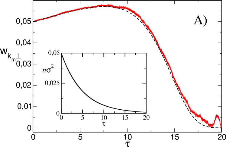
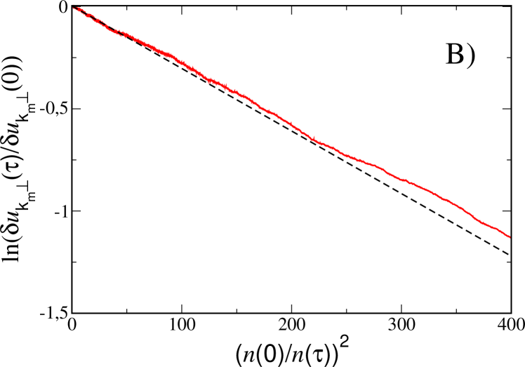
Figure 1: A) Time evolution of a linear perturbation of the transversal velocity for a system with annihilation probability $p=0.1$. The solid lines are the Molecular Dynamics results and the dashed lines are the theoretical predictions (no adjustable parameter). Note how the theoretical predictions correctly account for the increase of the perturbation at short times. The inset shows the evolution of density with rescaled time $\tau$, where $\sigma$ is the discs’ radius. For $\tau=20$, $n\sigma^{2}\simeq 9.10^{-4}$. B) Evolution of $\delta u_{\mathbf{k}\perp}(\tau)/\delta u_{\mathbf{k}\perp}(0)$ as a function of $n^{2}(0)/n^{2}(\tau)$. The dashed line is the exponential decay predicted by Eq. (96). $n^{2}(0)/n^{2}(\tau)=400$ corresponds to $\tau\simeq 15$.

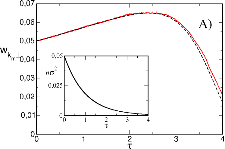
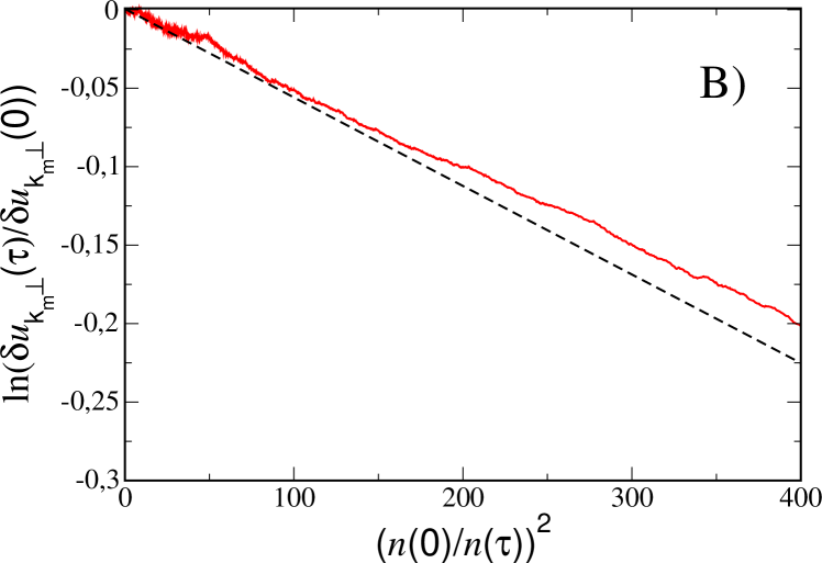
Figure 2: A) Same as in Fig. 1 but for a system with $p=0.5$, which –loosely speaking– may therefore be considered as being more “distant” to equilibrium. The inset shows the evolution of density with rescaled time $\tau$. For $\tau=4$, the rescaled density is $n\sigma^{2}\simeq 9.10^{-4}$ (while $n(0)\sigma^{2}=0.05$). B) Evolution of $\delta u_{\mathbf{k}\perp}(\tau)/\delta u_{\mathbf{k}\perp}(0)$ as a function of $n^{2}(0)/n^{2}(\tau)$. $n^{2}(0)/n^{2}(\tau)=400$ corresponds to $\tau\simeq 3$.

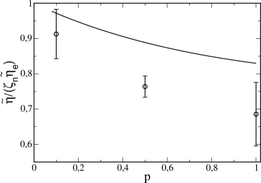
Figure 3: Symbols: ratio $\tilde{\eta}/\zeta_{n}$ (normalized by its $p\to 0$ value) extracted from the exponential fit of $\delta u_{\mathbf{k}\perp}(\tau)$ to Eq. (96). The solid line is the theoretical prediction in the first Sonine approximation.

V.1 Perturbation of the transversal velocity

Since Eq. (84) for the shear mode is decoupled from the other equations, one of the simplest macroscopic perturbation one can think of consists in an initial harmonic perturbation of the transversal component of the velocity field, whose evolution is given by Eq. (88). We shall consider a small perturbation in real space of the form

$$u_{x}(\mathbf{r},0)=A\sin(k_{m}y),$$ (95)

with $A=10^{-1}v_{H}(0)$ and $k_{m}=2\pi/L$, where $L$ is the linear size of the system. The reason for choosing the smallest possible value of $k$ compatible with the boundary conditions is twofold. First, the corresponding mode is the most unstable at short times (see Eq. (88)). For the parameters of the simulations, we indeed probe the region where $p\zeta_{T}>\tilde{\eta}\tilde{k}^{2}$, so that the hydrodynamic equation (88) predicts an initial increase of the perturbation. Second, the low $k$ regime is that where our large scale predictions are most likely to be relevant.

Figure 1 displays the evolution of $w_{k_{m}\perp}$ as a function of the number of collisions per particle $\tau$ for a system with $p=0.1$, averaging data over $50$ different trajectories. The solid line is the simulation result and the dashed line is the theoretical prediction, Eq. (88), where the shear viscosity and the decay rates have been computed using the standard tools of kinetic theory (here, the first Sonine approximation cdt04 , see Appendix A). An excellent agreement is obtained without any adjustable parameter, including the predicted increase of the perturbation at short times, and as also observed for a larger annihilation probability $p=0.5$ (see Fig. 2, in which the MD data are obtained by an average over $150$ runs).

Recalling that $n_{H}(\tau)/n_{H}(0)=\exp(-2p\zeta_{n}\tau)$ and that $v_{H}(\tau)=v_{H}(0)\exp(-p\zeta_{T}\tau)$, it proves also convenient to consider the actual velocity field $\delta\mathbf{u}(\tau)=v_{H}(\tau)\mathbf{w}(\tau)$ instead of its dimensionless counterpart $\mathbf{w}$, since the prediction (88) then takes the form :

$$\delta u_{\mathbf{k}\perp}(\tau)=\exp\left\{-\frac{\tilde{\eta}\tilde{k}^{2}}{4p\zeta_{n}}\left[\frac{n_{H}^{2}(0)}{n_{H}^{2}(\tau)}-1\right]\right\}\delta u_{\mathbf{k}\perp}(0).$$ (96)

The plot of $\delta u_{\mathbf{k}\perp}(\tau)/\delta u_{\mathbf{k}\perp}(0)$ as a function of $(n_{H}(0)/n_{H}(\tau))^{2}$ allows then by simple exponential fitting to extract $\tilde{\eta}/\zeta_{n}$ (recall that $\tilde{k}=l_{H}(0)k$ is known). Figure 3 compares the ratios $\tilde{\eta}/\zeta_{n}$ extracted from such fits for various values of $p$ with the theoretical prediction. We have plotted the value of the viscosity normalized by its elastic value, $\tilde{\eta}_{e}$. For $p=0.1$ the agreement is quite good but for $p=1$ we obtain discrepancies of the order of $15\%$. Such deviations could be due to the limitation for high dissipation of the first Sonine approximation that has been used to compute the numerical values of the various quantities involved in the description (in particular, the deviations of the homogeneous decay state velocity distribution from its Gaussian form might be relevant). Additionally, the shear viscosity could suffer from finite size effects. For a related discussion in the realm of granular gases, where both effects alluded to are at work, see msg07 ; gsm07 ; bgm08 . Finally, neglecting the $k^{2}$ contribution to $\delta\zeta_{\mathbf{u}}$ might not be innocuous. From symmetry considerations, such a term must be of the form $k^{2}l_{H}(\tau)^{2}\mathbf{w}_{\mathbf{k}}$, so that the equation (84) for the transversal velocity has the same form as the one we considered, but with a “shifted” shear viscosity. It is worth pointing out here that in the corresponding equation (88), putative order $k^{2}$ corrections to $\delta\zeta_{n}$ and $\delta\zeta_{T}$ play no role (see Eq. (84)) : the decay rates $\zeta_{n}$ and $\zeta_{T}$ appearing in (88) are fingerprints of the $\tau$ dependence of $l_{H}$ and of the rescaling procedure leading to $\mathbf{w}_{\mathbf{k}}$ from the actual velocity flow. Those two decay rates are therefore properties of the homogeneous solution and do not suffer any finite $k$ correction.

V.2 Perturbation of the longitudinal velocity

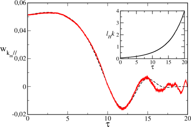
Figure 4: Time evolution of the longitudinal velocity for a system with $p=0.1$ as a function of $\tau$. The solid line shows the simulation results and the dashed line is the numerical solution of (89). For $\tau=15$ the rescaled density is $n\sigma^{2}\simeq 2.5.10^{-3}$. The inset shows the increase of mean-free path with time and that for $\tau>10$, $l_{H}k$ is no longer a small quantity.

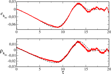
Figure 5: Time evolution of $e_{\mathbf{k_{m}}}$ and $\rho_{\mathbf{k_{m}}}$ as a function of $\tau$ for a system with $p=0.1$. The solid lines show Molecular Dynamics results while the dashed lines are for the numerical solution of (89). For $\tau=15$ the rescaled density is $n\sigma^{2}\simeq 2.5.10^{-3}$.

In order to investigate further the validity of the hydrodynamic equations, we consider a perturbation of the longitudinal velocity

$$u_{x}(\mathbf{r},0)=A\sin(k_{m}x),$$ (97)

where $A=10^{-1}v_{H}(0)$ and $k_{m}=2\pi/L$. Since the hydrodynamic matrix $M$ depends on time and $\frac{dM}{dt}$ does not commute with $M$, we could not solve analytically the set of equations (89), and we turned to a numerical integration, using the transport coefficients computed in Appendix A.

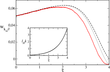
Figure 6: Time evolution of the longitudinal velocity for a system with $p=0.5$ as a function of $\tau$. The solid line shows the simulation results and the dashed line is for the numerical solution. We have also plotted with a dotted line the numerical solution considering the elastic values of $\tilde{\kappa}$ and $\tilde{\mu}$ (i.e. their limit when $p\to 0^{+}$). The inset shows the increase of mean-free path with time.

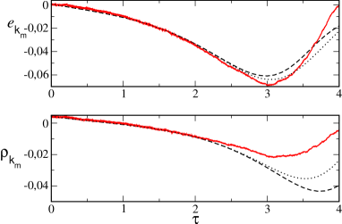
Figure 7: Time evolution of $e_{\mathbf{k_{m}}}$ and $\rho_{\mathbf{k_{m}}}$ as a function of $\tau$ for a system with $p=0.5$. The different lines have the same meaning as in Fig. 6.

In Fig. 4, we have plotted the time evolution of the rescaled longitudinal velocity field, $w_{k_{m}\parallel}$, as a function of the internal time clock $\tau$ (number of collisions per particle) for a system with $p=0.1$. The results have been averaged over $16$ trajectories. It can be seen that the theoretical framework is able to account for the non trivial time dependence of the perturbation dynamics. Moreover, as the equations for $\theta_{k_{m}}$ and $\rho_{k_{m}}$ are coupled with the equation for $w_{k_{m}\parallel}$, a perturbation such as (97) induces a response of the above two other fields (at variance with the transversal velocity, whose dynamics is decoupled from the other three modes, at least at the linear level of description adopted here). In Fig. 5, we have plotted the energy density $e_{k_{m}}=\theta_{k_{m}}+\rho_{k_{m}}$ and $\rho_{k_{m}}$ as a function of $\tau$. The agreement with theory is very good both qualitatively and quantitatively, with an evolution that is well predicted till $\tau\simeq 15$ ; for long times the simulation data become somewhat noisy (less statistics can be achieved due to the smaller number of particles left in the system. The number of particles at $\tau=15$ is $N\simeq 5000$).

In Fig.s 6 and 7, results for a system with $p=0.5$ are shown. Data are averaged over $64$ runs. In this case, the agreement is still good qualitatively, with similar shapes for the theoretical and numerical curves, but some discrepancies are observed. The most significant deviation from the theoretical prediction occurs for the density, $\rho_{k_{m}}$, where the value of the minimum and also its position are not predicted accurately. However, the hydrodynamic framework still captures correctly the trends of the complex dynamics of the perturbations. The above discrepancies could be ascribable to the failure of the first Sonine approximation for high dissipation (i.e. “high” $p$) or to finite size effects. We mention here that within the first Sonine approximation, the dimensionless coefficients $\tilde{\mu}$ and $\tilde{\kappa}$ exhibit a divergent behavior in the vicinity of $p=0.8$ cdt04 which is presumably unphysical, and is an indication of the limitation of the method. For completeness and to assess the robustness of the predictions with respect to a modification of the numerical values of the key parameters, we have also reported in Fig.s 6 and 7 the predictions obtained when the transport coefficients take their elastic hard disc value (e.g. $\tilde{\mu}(p=0.5)\simeq 0.505$ while $\tilde{\mu}(p=0)=0$, as required by Fourier’s law ). The important point is that the time evolutions are not significantly affected, and that the main features remain the same. Additionally, as mentioned after Eq. (66) and (96), a possible source of inaccuracy lies in the truncation of decay rates to their first order ($k^{1}$) in the gradients. While the corresponding terms have been shown to be small for inelastic hard spheres bdks98 (with the notable simplification there that the velocity decay rate vanishes identically due to momentum conservation), their relevance in the present case has not been assessed, apart indirectly for the velocity decay rate $\delta\bm{\zeta}_{u}$, by noting that second order corrections do not spoil the accuracy of the prediction (88), see Figures 1 and 2.

VI Conclusions

The objective here has been to explore the validity of a hydrodynamic description based on density, momentum, and kinetic temperature fields for a gas composed of particles which annihilate with probability $p$ or scatter elastically otherwise, by a direct analysis of the spectrum of the linear Boltzmann equation. The motivation mainly was to study the applicability of hydrodynamics to systems which a priori lack scale separation and in which there are no collisional invariants. The analysis performed here has been shown to lead to results equivalent to those obtained previously from the more formal Chapman-Enskog expansion cdt04 , with the difference that the present approach considers linear excitations only. However, the current spectral method is arguably more straightforward and explicitly shows that the hydrodynamic description arises in the appropriate time scale, when the “kinetic modes” can be considered as negligible against the hydrodynamic ones.

The eigenvalue problem of the Boltzmann operator linearized around the homogeneous decay state has been addressed and we have identified the hydrodynamic eigenfunctions. These eigenfunctions are not simply linear combinations of $1$, $\mathbf{v}$ and $v^{2}$ as it happens in the elastic case, but they are replaced by derivatives of the homogeneous decay state velocity distribution function $\chi_{H}$, that is not known analytically. As a consequence of the non-hermitian character of the linearized Boltzmann operator, the eigenfunctions are not orthogonal. It is nevertheless possible to construct a set of biorthonormal functions, $\{\bar{\xi}_{\beta}\}_{\beta=1,\ldots 3}$, which are linear combinations of $1$, $\mathbf{v}$ and $v^{2}$, a crucial point in order to obtain the hydrodynamic equations. The analysis is complicated by the fact that none of the $\{\bar{\xi}_{\beta}\}$ functions are left eigenfunctions of the linearized Boltzmann operator, since no quantity is conserved during binary encounters. We have used these hydrodynamic eigenfunctions to derive to Navier-Stokes order the heat and momentum fluxes, together with the various decay rates. To this end, we have decomposed the distribution function, $\delta\chi_{\mathbf{k}}$, into its hydrodynamic and non-hydrodynamic parts. This decomposition enables us to close the hydrodynamic equations in the long time limit and to order $k^{2}$, and provides Green-Kubo formulas for the transport coefficients. We then arrived at the linearized equations (around the homogeneous decay state) for the hydrodynamic fields, in the usual form of partial differential equations with coefficients that are independent of the space variable but depend on time, since the reference state considered is itself time dependent. If we analyze the stability of these equations, we may conclude that small perturbations should decay in the long time limit. Nevertheless, it must be stressed that the perturbation may increase at short times, thereby possibly leaving the linear domain where our analysis holds. The long time dynamics in such a case remains an open question.

In section V, we have reported Molecular Dynamics simulations for the evolution of a perturbation of the transversal and longitudinal velocity fields, which show a rich dynamics. The agreement between theory and simulations is very good for moderate values of the annihilation probability $p$ (say $p<0.5$), which gives strong support to the theoretical analysis developed here. The theoretical curves still agree qualitatively at larger $p$, with however some quantitative discrepancies which might be a manifestation of the approximations underlying the computation of the transport coefficients (namely $\kappa$ and $\mu$, evaluated to first order in a Sonine expansion cdt04 ). Indeed, those coefficients are predicted to exhibit a divergent behavior for $p\sim 0.8$, but the simulations we have performed do not show a qualitatively different behavior for these values of $p$. A further complication –that is also an a priori limitation for the efficiency of a hydrodynamic approach– is that for values of $p$ close to unity, the separation of time scales between the kinetic and hydrodynamic modes is not clear cut (the density decay rate is on the order of the collision frequency, comparable to the inverse typical time of the kinetic modes). To address this concern, one should study in detail the spectrum of non hydrodynamic modes to find the slowest, and compare it to the fastest decay rate in our problem (i.e. $\zeta_{n}$). Such a program, left for future work, has been achieved in Appendix C within the Maxwell model framework, with the conclusion that scale separation does not hold for $p>p^{*}=1/4$. While the threshold $p^{*}$ is a priori model dependent, a similar phenomenon is to be expected in the original “hard-sphere” dynamics considered in this paper. The coarse-grained description for $p>p^{*}$ is an open question.

Appendix A Approximate expression for the transport coefficients and decay rates

For completeness, we recall here the explicit expressions used for the transport coefficients and decay rates, as obtained within the first order Sonine scheme in Ref. cdt04 . The distribution function in this approximation reads

$$\chi_{H}(c)=\frac{1}{\pi^{d/2}}e^{-c^{2}}\left\{1+a_{2}\left[\frac{d(d+2)}{8}-\frac{d+2}{2}c^{2}+\frac{c^{4}}{2}\right]\right\},$$ (98)

with the kurtosis

$$a_{2}=\frac{8(3-2\sqrt{2})p}{(4d+6-\sqrt{2})p+8\sqrt{2}(d-1)(1-p)}.$$ (99)

This expression allows us to calculate the decay rates

$$\zeta_{n} = \frac{d+2}{4}\left(1-a_{2}\frac{1}{16}\right),$$ (100)

$$\zeta_{T} = \frac{d+2}{8d}\left(1+a_{2}\frac{8d+11}{16}\right),$$ (101)

and also the transport coefficients

$$\tilde{\eta}=\frac{1}{4\nu_{\eta}-2p\zeta_{T}},$$ (102)

$$\tilde{\kappa}=\frac{1}{\nu_{\kappa}-2p\zeta_{T}}\left[\frac{1}{2}p\zeta_{n}\tilde{\mu}+\frac{d+2}{8}(2a_{2}+1)\right],$$ (103)

$$\tilde{\mu}=\frac{1}{2\nu_{\kappa}-3p\zeta_{T}-2p\zeta_{n}}\left[p\zeta_{T}\tilde{\kappa}+\frac{d+2}{8}(2a_{2}+1)\right],$$ (104)

where the values of the coefficients $\nu_{\eta}$ and $\nu_{\kappa}$ are

$$\nu_{\eta}=\frac{p}{8d}\left[3+6d+2d^{2}-a_{2}\frac{278+375d+96d^{2}+2d^{3}}{32(d+2)}\right]+(1-p)\left(1-a_{2}\frac{1}{32}\right),$$ (105)

$$\nu_{\kappa}=\frac{p}{32d}\left[16+27d+8d^{2}+a_{2}\frac{2880+1544d-2658d^{2}-1539d^{3}-200d^{4}}{32d(d+2)}\right]+(1-p)\frac{d-1}{d}\left(1+a_{2}\frac{1}{32}\right).$$ (106)

Finally, the expressions for $\zeta_{u,\rho}$ and $\zeta_{u,\theta}$ are

$$\zeta_{u,\rho} = \frac{8(d-1)}{d(d+2)}\tilde{\mu}\zeta_{u},$$ (107)

$$\zeta_{u,\theta} = \frac{8(d-1)}{d(d+2)}\tilde{\kappa}\zeta_{u},$$ (108)

with

$$\zeta_{u}=\frac{(d+2)^{2}}{32(d-1)}\left[1+a_{2}\frac{-86-101d+32d^{2}+88d^{3}+28d^{4}}{32(d+2)}\right].$$ (109)

Appendix B Eigenfunctions of $\Lambda$

In this Appendix some of the details leading to the solution of the eigenvalue problem (41) are given. Consider first the function

$$\Psi_{1}(\mathbf{c})=\chi_{H}(\mathbf{c}).$$ (110)

and let the linearized operator $\Lambda$ act onto $\chi_{H}$

$$\Lambda(\mathbf{c}_{1})\chi_{H}(\mathbf{c}_{1}) = \gamma\int\!\!d\mathbf{c}_{2}T(\mathbf{c}_{1},\mathbf{c}_{2})(1+{\cal P}_{12})\chi_{H}(\mathbf{c}_{1})\chi_{H}(\mathbf{c}_{2})$$ (111)

$$+ p(2\zeta_{n}-d\zeta_{T})\chi_{H}(\mathbf{c}_{1})-p\zeta_{T}\mathbf{c}_{1}\cdot\frac{\partial}{\partial\mathbf{c}_{1}}\chi_{H}(\mathbf{c}_{1}).$$

If we take into account the equation for $\chi_{H}(\mathbf{c}_{1})$

$$(d\zeta_{T}-2\zeta_{n})p\chi_{H}(\mathbf{c}_{1})+p\zeta_{T}\mathbf{c}_{1}\cdot\frac{\partial}{\partial\mathbf{c}_{1}}\chi_{H}(\mathbf{c}_{1})=\gamma\int\!\!d\mathbf{c}_{2}T(\mathbf{c}_{1},\mathbf{c}_{2})\chi_{H}(\mathbf{c}_{1})\chi_{H}(\mathbf{c}_{2}),$$ (112)

we can rewrite equation (111) as

$$\Lambda(\mathbf{c}_{1})\chi_{H}(\mathbf{c}_{1})=(d\zeta_{T}-2\zeta_{n})p\chi_{H}(\mathbf{c}_{1})+p\zeta_{T}\mathbf{c}_{1}\cdot\frac{\partial}{\partial\mathbf{c}_{1}}\chi_{H}(\mathbf{c}_{1}).$$ (113)

Consider now the function

$$\Psi_{2}(\mathbf{c})=\mathbf{c}\cdot\frac{\partial}{\partial\mathbf{c}}\chi_{H}(\mathbf{c}).$$ (114)

In order to proceed, we perform the change of variables $\mathbf{c}_{1}=\lambda\mathbf{c}_{1}^{\prime}$ in equation (112)

$$(d\zeta_{T} - 2\zeta_{n})p\chi_{H}(\lambda\mathbf{c}_{1}^{\prime})+p\zeta_{T}\mathbf{c}_{1}^{\prime}\cdot\frac{\partial}{\partial\mathbf{c}_{1}^{\prime}}\chi_{H}(\lambda\mathbf{c}_{1}^{\prime})$$

$$= \gamma\lambda^{d+1}\int\!\!d\mathbf{c}_{2}^{\prime}\!\!\int\!\!d\hat{\bm{\sigma}}\theta(\mathbf{c}_{12}^{\prime}\cdot\hat{\bm{\sigma}})\mathbf{c}_{12}^{\prime}\cdot\hat{\bm{\sigma}}[(1-p)b_{\bm{\sigma}}^{-1}-1]\chi_{H}(\lambda\mathbf{c}_{1}^{\prime})\chi_{H}(\lambda\mathbf{c}_{2}^{\prime}).$$

Deriving with respect to $\lambda$ we obtain

$$(d\zeta_{T}-2\zeta_{n})p\frac{\partial}{\partial\lambda}\chi_{H}(\lambda\mathbf{c}_{1}) + p\zeta_{T}\mathbf{c}_{1}\cdot\frac{\partial}{\partial\mathbf{c}_{1}}\left(\frac{\partial}{\partial\lambda}\chi_{H}(\lambda\mathbf{c}_{1})\right)$$ (116)

$$= (d+1)\lambda^{d}\gamma\int\!\!d\mathbf{c}_{2}T(\mathbf{c}_{1},\mathbf{c}_{2})\chi_{H}(\lambda\mathbf{c}_{1})\chi_{H}(\lambda\mathbf{c}_{2})$$

$$+ \gamma\lambda^{d+1}\int\!\!d\mathbf{c}_{2}T(\mathbf{c}_{1},\mathbf{c}_{2})\frac{\partial\chi_{H}(\lambda\mathbf{c}_{1})}{\partial\lambda}\chi_{H}(\lambda\mathbf{c}_{2})$$

$$+ \gamma\lambda^{d+1}\int\!\!d\mathbf{c}_{2}T(\mathbf{c}_{1},\mathbf{c}_{2})\chi_{H}(\lambda\mathbf{c}_{1})\frac{\partial\chi_{H}(\lambda\mathbf{c}_{2})}{\partial\lambda}.$$

and taking $\lambda=1$ we arrive at the equation for $\Psi_{2}(\mathbf{c})$

$$(d\zeta_{T}-2\zeta_{n})p\Psi_{2}(\mathbf{c}_{1}) + p\zeta_{T}\mathbf{c}_{1}\cdot\frac{\partial}{\partial\mathbf{c}_{1}}\Psi_{2}(\mathbf{c}_{1})$$ (117)

$$= (d+1)\gamma\int\!\!d\mathbf{c}_{2}T(\mathbf{c}_{1},\mathbf{c}_{2})\chi_{H}(\lambda\mathbf{c}_{1})\chi_{H}(\lambda\mathbf{c}_{2})$$

$$+ \gamma\int\!\!d\mathbf{c}_{2}T(\mathbf{c}_{1},\mathbf{c}_{2})\Psi_{2}(\mathbf{c}_{1})\chi_{H}(\lambda\mathbf{c}_{2})$$

$$+ \gamma\int\!\!d\mathbf{c}_{2}T(\mathbf{c}_{1},\mathbf{c}_{2})\chi_{H}(\lambda\mathbf{c}_{1})\Psi_{2}(\mathbf{c}_{2}),$$

or equivalently

$$\Lambda(\mathbf{c}_{1})\Psi_{2}(\mathbf{c}_{1})=-(d+1)\left[(d\zeta_{T}-2\zeta_{n})p\chi_{H}(\mathbf{c}_{1})+p\zeta_{T}\mathbf{c}_{1}\cdot\frac{\partial}{\partial\mathbf{c}_{1}}\chi_{H}(\mathbf{c}_{1})\right].$$ (118)

Consequently, equations (113) and (118) can be written as

$$\Lambda(\mathbf{c}_{1})\Psi_{1}(\mathbf{c}_{1}) = (d\zeta_{T}-2\zeta_{n})p\Psi_{1}(\mathbf{c}_{1})+p\zeta_{T}\Psi_{2}(\mathbf{c}_{1}),$$ (119)

$$\Lambda(\mathbf{c}_{1})\Psi_{2}(\mathbf{c}_{2}) = -(d+1)[(d\zeta_{T}-2\zeta_{n})p\Psi_{1}(\mathbf{c}_{1})+p\zeta_{T}\Psi_{2}(\mathbf{c}_{1})].$$ (120)

With equations (119) and (120) we can easily see that

$$\Lambda(\mathbf{c}_{1})[(d+1)\Psi_{1}(\mathbf{c}_{1})+\Psi_{2}(\mathbf{c}_{1})]=0,$$ (121)

so that

$$\xi_{1}(\mathbf{c}_{1})\equiv(d+1)\Psi_{1}(\mathbf{c}_{1})+\Psi_{2}(\mathbf{c}_{1}),$$ (122)

is an eigenfunction of the operator $\Lambda(\mathbf{c}_{1})$ with eigenvalue $\lambda_{1}=0$. It is also straightforward to see that

$$\xi_{2}(\mathbf{c}_{1})=(d\zeta_{T}-2\zeta_{n})p\Psi_{1}(\mathbf{c}_{1})+p\zeta_{T}\Psi_{2}(\mathbf{c}_{1}),$$ (123)

is an eigenfunction of $\Lambda$. We obtain that

$$\Lambda(\mathbf{c}_{1})\xi_{2}(\mathbf{c}_{1}) = (d\zeta_{T}-2\zeta_{n})p\Lambda(\mathbf{c}_{1})\Psi_{1}(\mathbf{c}_{1})+p\zeta_{T}\Lambda(\mathbf{c}_{1})\Psi_{2}(\mathbf{c}_{1})$$ (124)

$$= -(\zeta_{T}+2\zeta_{n})p\xi_{2}(\mathbf{c}_{1}),$$

where we have used equations (119) and (120). Therefore, we have that $\xi_{2}(\mathbf{c}_{1})$ is an eigenfunction of $\Lambda(\mathbf{c}_{1})$ with eigenvalue $\lambda_{2}=-(\zeta_{T}+2\zeta_{n})p$.

Finally, let us consider the last function

$$\bm{\Psi}_{3}(\mathbf{c})=-\frac{\partial}{\partial\mathbf{c}}\chi_{H}(\mathbf{c}).$$ (125)

Deriving the equation obeyed by $\chi_{H}(\mathbf{c}-\mathbf{w})$, with respect to $\mathbf{w}$ and subsequently evaluating the result for $\mathbf{w}=\mathbf{0}$, we obtain

$$(d\zeta_{T}-2\zeta_{n})p\bm{\Psi}_{3}(\mathbf{c}_{1}) + p\zeta_{T}\bm{\Psi}_{3}(\mathbf{c}_{1})+p\zeta_{T}\mathbf{c}_{1}\cdot\frac{\partial}{\partial\mathbf{c}_{1}}\bm{\Psi}_{3}(\mathbf{c}_{1})$$ (126)

$$= \gamma\int\!\!d\mathbf{c}_{2}T(\mathbf{c}_{1},\mathbf{c}_{2})(1+{\cal P}_{12})\bm{\Psi}_{3}(\mathbf{c}_{1})\chi_{H}(\mathbf{c}_{2}),$$

or equivalently

$$\Lambda(\mathbf{c}_{1})\bm{\Psi}_{3}(\mathbf{c}_{1})=p\zeta_{T}\bm{\Psi}_{3}(\mathbf{c}_{1}).$$ (127)

In other words, $\bm{\xi}_{3}(\mathbf{c}_{1})\equiv\bm{\Psi}_{3}(\mathbf{c}_{1})$ is an eigenfunction of $\Lambda(\mathbf{c}_{1})$ with eigenvalue $\lambda_{3}=p\zeta_{T}$.

Appendix C Linearized Boltzmann operator for Maxwell Molecules

The objective in this Appendix is to study the spectrum of the linearized Boltzmann operator for Maxwell molecules with annihilation. It will be shown that for $0\leq p\leq p^{*}$, where $p^{*}$ depends on the specific Maxwell model under consideration, the norm of the hydrodynamic eigenvalues are smaller than the rest of the spectrum.

The main characteristic of Maxwell models is that the differential cross section multiplied by the relative velocity is independent of the relative velocity. We are going to assume that it is also independent of the angle between the two colliding particles. Then, the Boltzmann equation for a system of Maxwell molecules which annihilate in a collision with probability $p$ and collide elastically otherwise (with probability $1-p$) reads

$$\left(\frac{\partial}{\partial t}+\mathbf{v}_{1}\cdot\nabla\right)f(\mathbf{r},\mathbf{v}_{1},t) = -p\beta\Omega\int\!\!d\mathbf{v}_{2}f(\mathbf{r},\mathbf{v}_{1},t)f(\mathbf{r},\mathbf{v}_{2},t)$$

$$+ (1-p)\beta\int\!\!d\mathbf{v}_{2}\!\!\int\!\!d\hat{\bm{\sigma}}[b_{\sigma}^{-1}-1]f(\mathbf{r},\mathbf{v}_{1},t)f(\mathbf{r},\mathbf{v}_{2},t),$$

where $\beta$ is a constant representing the microscopic scattering collision frequency, $\Omega=2\pi^{d/2}/\Gamma(d/2)$ is the $d$-dimensional solid angle and the operator $b_{\sigma}^{-1}$ is defined in the main text, Eq. (4).

If we consider the homogeneous case, it is straightforward to see that the temperature is a constant in time, $T_{H}(t)=T_{H}(0)$, and that the density evolves as

$$n_{H}(t)=\frac{n_{H}(0)}{1+p\zeta_{n}t},$$ (129)

with $\zeta_{n}=\beta\Omega n_{H}(0)$. Moreover, it was shown in commentsb85 that there is an exact mapping between the homogeneous equation for Maxwell molecules with annihilation (arbitrary $p$) and the usual elastic Maxwell molecules ($p=0$). If we introduce the time scale

$$s(t)=\int_{0}^{t}dt^{\prime}\frac{n_{H}(t^{\prime})}{n_{H}(0)},$$ (130)

it can be seen that the distribution function for arbitrary $p$ is

$$f(\mathbf{v},t)=\frac{n_{H}(t)}{n_{H}(0)}f^{E}\left[\mathbf{v},(1-p)s(t)\right],$$ (131)

where $n_{H}(t)$ is given by formula (129), $s(t)$ by (130), and the function $f^{E}$ is the distribution function for elastic Maxwell molecules. Note that this relation is also valid for $p=1$ where $f^{E}$ is frozen in the initial condition.

In the elastic case, every homogeneous distribution tends to relax to a Maxwellian after a transient time. Then, the same is going to happen for arbitrary $p<1$ because of the mapping. In this sense, we can consider that the state analogous to the homogeneous decay state introduced in the main text for hard particles and that will constitute the appropriate reference will be characterized by the distribution function

$$f_{H}(\mathbf{v},t)=\frac{n_{H}(t)}{v_{H}^{d}}\chi_{M}(v/v_{H}),$$ (132)

where $v_{H}=\left(\frac{2T_{H}}{m}\right)^{1/2}$ and $\chi_{M}(v)=1/\pi^{d/2}e^{-v^{2}}$ is the Maxwellian distribution. Note that in the homogeneous decay state, both the density and temperature decay, whether in the present case only the density decays. Then, as $v_{H}$ plays no role, we will consider units with $v_{H}=1$ for simplicity.

Let us study now the linear response to an inhomogeneous small perturbation around the reference state as it was done in section II. If we introduce the scaled distribution function

$$\delta\chi(\mathbf{r},\mathbf{v},\tau)=\frac{n_{H}(0)}{n_{H}(t)}[f(\mathbf{r},\mathbf{v},t)-f_{H}(\mathbf{v},t)],$$ (133)

the equation for $\delta\chi$ in the $s$ scale defined in (130) is

$$\left[\frac{\partial}{\partial s}+h_{H}(s)\mathbf{v}_{1}\cdot\nabla\right]\delta\chi(\mathbf{r},\mathbf{v},s)=\Lambda(\mathbf{v}_{1})\delta\chi(\mathbf{r},\mathbf{v},s),$$ (134)

where we have introduced the function $h_{H}(s)=n_{H}(0)/n_{H}(s)$, and the linearized Boltzmann operator

$$\Lambda(\mathbf{v}_{1})g(\mathbf{v}_{1}) = (1-p)\frac{\zeta_{n}}{\Omega}\int\!\!d\mathbf{v}_{2}\!\!\int\!\!d\hat{\bm{\sigma}}[b_{\sigma}^{-1}-1](1+{\cal P}_{12})\chi_{M}(v_{1})g(\mathbf{v}_{2})$$ (135)

$$- p\zeta_{n}\chi_{M}(v_{1})\int\!\!d\mathbf{v}_{2}g(\mathbf{v}_{2}).$$

Let us stress that, although there is an exact mapping for the full non-linear homogeneous equation between $p=0$ and arbitrary $p$, no such mapping exists for the linear inhomogeneous Boltzmann equation, Eq. (134). Then, as in the main text, the possibility of an hydrodynamic description depends on the properties of the linearized Boltzmann operator. Here we will see that it is possible to calculate all the eigenfunctions and eigenvalues of this operator and that there is a region of the parameter $p$ in which we have an appropriate scale separation.

Let us write the linearized Boltzmann operator as

$$\Lambda(\mathbf{v}_{1})g(\mathbf{v}_{1})=(1-p)\Lambda^{E}(\mathbf{v}_{1})g(\mathbf{v}_{1})-p\zeta_{n}\chi_{M}(v_{1})\int\!\!d\mathbf{v}_{2}g(\mathbf{v}_{2}),$$ (136)

where we have introduced the linearized Boltzmann operator for elastic Maxwell particles

$$\Lambda^{E}(\mathbf{v}_{1})=\frac{\zeta_{n}}{\Omega}\int\!\!d\mathbf{v}_{2}\!\!\int\!\!d\hat{\bm{\sigma}}[b_{\sigma}^{-1}-1](1+{\cal P}_{12})\chi_{M}(v_{1})g(\mathbf{v}_{2}),$$ (137)

whose spectral properties are well known resibois ; mclennan . In particular, for $d=3$ its eigenfunctions are

$$\phi_{rlm}(\mathbf{v})=A_{rl}\chi_{M}(v)S^{r}_{l+1/2}(v^{2})v^{l}Y_{lm}(\theta,\varphi),\qquad r=0,1,\dots$$ (138)

where $Y_{lm}(\theta,\varphi)$ are the spherical harmonics, functions of the polar angles $(\theta,\varphi)$ of $\mathbf{v}$ with respect to an arbitrary direction, $S^{r}_{l+1/2}(v^{2})$ are the Sonine polynomials which satisfy

$$\int_{0}^{\infty}dxe^{-x}S^{n}_{q}(x)S^{n^{\prime}}_{q}(x)=\frac{\Gamma(n+q+1)}{n!}\delta_{nn^{\prime}},$$ (139)

and $A_{rl}$ are some constants that are introduced in order to normalize the eigenfunctions and that play no role in the following analysis. The eigenvalues of $\Lambda^{E}$, $\lambda^{E}_{rl}$, are also known. It can be seen that $\lambda^{E}_{00}$, $\lambda^{E}_{10}$, and $\lambda^{E}_{01}$ (which is 3 times degenerate) vanish, corresponding to the five hydrodynamic eigenvalues and that the slowest kinetic mode corresponds to an eigenvalue $\lambda^{E}_{k}=-\zeta_{n}/3$.

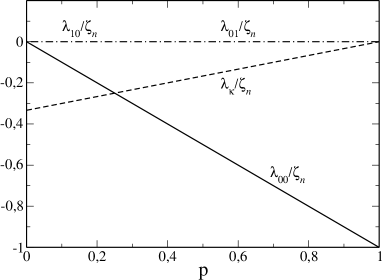
Figure 8: Hydrodynamic eigenvalues, $\lambda_{00}$, $\lambda_{10}$, and $\lambda_{01}$, and the slowest kinetic eigenvalue, $\lambda_{k}$, as a function of the dissipation parameter $p$. The eigenvalues are normalized by $\zeta_{n}=\beta\Omega n_{H}(0)$.

The important point here is that the functions $\phi_{rlm}$ are also eigenfunctions of the second operator in (136). Taking into account the orthogonality properties of the spherical harmonics and of the Sonine polynomials, Eq. (139), one has

$$\int\!\!d\mathbf{v}\phi_{rlm}(\mathbf{v})=\delta_{r0}\delta_{l0}.$$ (140)

Then, as $\phi_{000}(\mathbf{v})=\chi_{M}(v)$, the functions $\phi_{rlm}(\mathbf{v})$ are in fact the eigenfunctions of the total linearized Boltzmann operator for arbitrary $p$. With the aid of (140) is straightforward to see that the eigenvalues are

$$\lambda_{rl}=(1-p)\lambda^{E}_{rl}-p\zeta_{n}\delta_{r0}\delta_{l0}.$$ (141)

In Fig. 8 we plot the hydrodynamic eigenvalues as well as the slowest kinetic eigenvalue, $\lambda_{k}$, as a function of the dissipation parameter $p$. It can be seen that for $0\leq p<1/4$, there is scale separation in the sense that the three modes (density, linear momentum and kinetic energy) retained in the coarse-grained description decay slower that any of the other “kinetic” modes. On the other hand, for $1/4<p\leq 1$, the largest kinetic eigenvalue is slower than $\lambda_{00}$. We therefore conclude here that a conservative requirement for the validity of our approach in the case of Maxwell molecules would be $p<1/4$.

Appendix D Evaluation of $\delta\zeta_{n}$, $\delta\bm{\zeta}_{u}$ and $\delta\zeta_{T}$

In this Appendix we calculate the contribution of the hydrodynamic part of $\delta\chi_{\mathbf{k}}$ to the functionals $\delta\zeta_{n}$, $\delta\bm{\zeta}_{u}$ and $\delta\zeta_{T}$ defined in (38)-(40). To this end, we write explicitly $P\delta\chi_{\mathbf{k}}$ as

$$P\delta\chi_{\mathbf{k}}(\mathbf{c}_{1}) = \rho_{\mathbf{k}}\xi_{1}(\mathbf{c}_{1})+\left(\frac{1}{2}\theta_{\mathbf{k}}+\rho_{\mathbf{k}}\right)\xi_{2}(\mathbf{c}_{1})+\mathbf{w}_{\mathbf{k}}\cdot\bm{\xi}_{3}(\mathbf{c}_{1})$$ (142)

$$= \rho_{\mathbf{k}}\chi_{H}(\mathbf{c}_{1})-\frac{1}{2}\theta_{\mathbf{k}}\frac{\partial}{\partial\mathbf{c}_{1}}\cdot[\mathbf{c}_{1}\chi_{H}(\mathbf{c}_{1})]-\mathbf{w}_{\mathbf{k}}\cdot\frac{\partial}{\partial\mathbf{c}_{1}}\chi_{H}(\mathbf{c}_{1}).$$

Let us first evaluate $\delta\zeta_{n}[P\delta\chi_{\mathbf{k}}]$. After some algebra it can be seen that

$$\delta\zeta_{n}[\chi_{H}(\mathbf{c}_{1})] = -4\zeta_{n},$$ (143)

$$\delta\zeta_{n}\left[\frac{\partial}{\partial\mathbf{c}_{1}}\cdot[\mathbf{c}_{1}\chi_{H}(\mathbf{c}_{1})]\right] = 2\zeta_{n},$$ (144)

$$\delta\zeta_{n}\left[\frac{\partial}{\partial{\mathbf{c}_{1}}}\chi_{H}(\mathbf{c}_{1})\right] = 0,$$ (145)

where we have used equations (114), (117), the definition of the density decay rate, equation (14), and symmetry considerations. Then, if we consider equations (143)-(145) we finally obtain

$$\delta\zeta_{n}[P\delta\chi_{\mathbf{k}}]=-4\zeta_{n}\rho_{\mathbf{k}}-\zeta_{n}\theta_{\mathbf{k}}.$$ (146)

Now let us calculate $\delta\bm{\zeta}_{u}[P\delta\chi_{\mathbf{k}}]$. Using the definition of the density decay rate, equation (14), and symmetry considerations, it appears that

$$\delta\bm{\zeta}_{u}[\chi_{H}(\mathbf{c}_{1})] = 0,$$ (147)

$$\delta\bm{\zeta}_{u}\left[\frac{\partial}{\partial\mathbf{c}_{1}}\cdot(\mathbf{c}_{1}\chi_{H}(\mathbf{c}_{1}))\right] = 0,$$ (148)

$$\delta\zeta_{u_{i}}\left[\frac{\partial}{\partial c_{1j}}\chi_{H}(\mathbf{c}_{1})\right] = \delta_{ij}\delta\zeta_{u_{i}}\left[\frac{\partial}{\partial c_{1i}}\chi_{H}(\mathbf{c}_{1})\right]=2\zeta_{n}.$$ (149)

Then, we have

$$\delta\bm{\zeta}_{u}[P\delta\chi_{\mathbf{k}}]=-2\zeta_{n}\mathbf{w}_{\mathbf{k}}.$$ (150)

Finally, we turn to $\delta\zeta_{T}[P\delta\chi_{\mathbf{k}}]$. Using the definitions of the decay rates, equations (14) and (15), we obtain

$$\delta\zeta_{T}[\chi_{H}(\mathbf{c}_{1})] = -4\zeta_{T},$$ (151)

$$\delta\zeta_{T}\left[\frac{\partial}{\partial\mathbf{c}_{1}}\cdot(\mathbf{c}_{1}\chi_{H}(\mathbf{c}_{1}))\right] = 6\zeta_{T}+4\zeta_{n},$$ (152)

$$\delta\zeta_{T}\left[\frac{\partial}{\partial{\mathbf{c}_{1}}}\chi_{H}(\mathbf{c}_{1})\right] = 0$$ (153)

from which it follows that

$$\delta\zeta_{T}[P\delta\chi_{\mathbf{k}}]=-4\zeta_{T}\rho_{\mathbf{k}}-(3\zeta_{T}+2\zeta_{n})\theta_{\mathbf{k}}.$$ (154)

References

- (1) I. Goldhirsch, Ann. Rev. Fluid Mech. 35, 267 (2005).
- (2) J. Dufty, arXiv:0709.0479 (2007).
- (3) A. Barrat, E. Trizac, and M. H. Ernst, J. Phys.: Condens. Matter 17, S2429 (2005).
- (4) J. Brey and D. Cubero, in Granular gases, edited by S. Luding and T. Pöschel (Springer, Berlin, 2001).
- (5) E. Ben-Naim, P. Krapivsky, F. Leyvraz, and S. Redner, J. Chem. Phys. 98, 7284 (1994).
- (6) R. Blythe, M. R. Evans, and Y. Kafri, Phys. Rev. Lett. 85, 3759 (2000).
- (7) P. Krapivsky and C. Sire, Phys. Rev. Lett. 86, 2494 (2001).
- (8) E. Trizac, Phys. Rev. Lett. 88, 160601 (2002).
- (9) J. Piasecki, E. Trizac, and M. Droz, Phys. Rev. E 66, 066111 (2002).
- (10) A. Lipowski, D. Lipowska, and A. Feirrera, Phys. Rev. E 73, 032102 (2006).
- (11) S. Chapman and T. G. Cowling, The mathematical theory of nonuniform gases (Cambridge University Press, London, 1960).
- (12) F. Coppex, M. Droz, and E. Trizac, Phys. Rev. E 70, 061102 (2004).
- (13) J. J. Brey and M. J. Ruiz-Montero, Phys. Rev. E 69, 011305 (2004).
- (14) O. E. Lanford, Physica A 106, 70 (1981).
- (15) F. Coppex, M. Droz, and E. Trizac, Phys. Rev. E 69, 011303 (2004).
- (16) J. J. Brey, J. W. Dufty, and M. J. Ruiz-Montero, in Granular Gas Dynamics, edited by T. Pöschel and N. Brilliantov (Springer, Berlin, 2003).
- (17) J. J. Brey and J. W. Dufty, Phys. Rev. E 72, 011303 (2005).
- (18) J. Dufty, arXiv:0707.111, submitted to Journal of Physical Chemistry B (2007).
- (19) M. P. Allen and D. J. Tildesley, Computer Simulation of Liquids (Oxford Science Publications, Bristol, 1987).
- (20) J. M. Montanero, A. Santos, and V. Garzó, Physica A 376, 75 (2007).
- (21) V. Garzó, A. Santos, and J. M. Montanero, Physica A 376, 94 (2007).
- (22) J. J. Brey, M. I. García de Soria, and P. Maynar, (to be published).
- (23) J. J. Brey, J. W. Dufty, C. S. Kim, and A. Santos, Phys. Rev. E 58, 4638 (1998).
- (24) A. Santos and J. J. Brey, Phys. Fluids 29, 1750 (1986).
- (25) P. Résibois and M. de Leener, Classical Kinetic Theory of Fluids (John Wiley, New York, 1977).
- (26) J. A. McLennan, Introduction to Nonequilibrium Statistical Mechanics (Prentice-Hall, Englewood Cliffs, NJ, 1989).