Molecular structure of the $B_{s0}^{\ast}(5725)$ and $B_{s1}(5778)$ bottom-strange mesons

Abstract

We discuss a possible interpretation of the scalar $B_{s0}^{\ast}(5725)$ and axial $B_{s1}(5778)$ bottom–strange mesons as hadronic molecules — bound states of $BK$ and $B^{\ast}K$ mesons, respectively. Using a phenomenological Lagrangian approach we analyze the strong $B_{s0}^{\ast}\to B_{s}\pi^{0}$, $B_{s1}\to B_{s}^{\ast}\pi^{0}$ and the radiative $B_{s0}^{\ast}\to B_{s}^{\ast}\gamma$, $B_{s1}\to B_{s}\gamma$, $B_{s1}\to B_{s}^{\ast}\gamma$, $B_{s1}\to B_{s0}^{\ast}\gamma$ decays. We give predictions for the decay properties: effective couplings and decay widths.

I Introduction

Newly observed hadrons, in particular in the heavy flavor sector, have raised strong interest in treating and interpreting these states as hadronic bound states or, as commonly named, hadronic molecules (for overview see e.g. Ref. Rosner:2006vc ). One of the main reasons to treat these observed states as molecules is that their masses are close to the thresholds of corresponding hadronic pairs. Canonical examples are the scalar $D_{s0}^{\ast}(2317)$ and axial $D_{s1}(2460)$ mesons. As stressed in Barnes:2003dj the scalar $D_{s0}^{\ast}(2317)$ and axial $D_{s1}(2460)$ mesons could be candidates for a scalar $DK$ and a axial $D^{\ast}K$ molecule because of a relatively small binding energy of $\sim 50$ MeV.

In a series of papers Faessler:2007gv -Dong:2007px we developed the quantum field approach based on phenomenological Lagrangians for the treatment of hadrons as bound states of lighter hadrons — hadronic molecules. In particular, we considered the strong, radiative and leptonic decays of $D_{s0}^{\ast}(2317)$ and $D_{s1}(2460)$ mesons Faessler:2007gv -Faessler:2007us . A new feature related to the $DK$ and $D^{\ast}K$ molecular structure of the $D_{s0}^{\ast}$ and $D_{s1}$ mesons was that the presence of $u(d)$ quarks in the $D^{(\ast)}$ and $K$ mesons gives rise to direct strong isospin-violating transitions $D_{s0}^{\ast}\to D_{s}\pi^{0}$ and $D_{s1}\to D_{s}^{\ast}\pi^{0}$ in addition to the decay mechanism induced by $\eta-\pi^{0}$ mixing, as considered previously. We showed that the direct transition compares with and even dominates over the $\eta-\pi^{0}$ mixing transition in the isospin-violating decays of $D_{s0}^{\ast}$ and $D_{s1}$ mesons. The composite (molecular) structure of the $D_{s0}^{\ast}$ and $D_{s1}$ mesons was defined by the compositeness condition $Z=0$ Weinberg:1962hj ; Efimov:1993ei ; Anikin:1995cf (see also Refs. Baru:2003qq and Faessler:2007gv -Dong:2007px ). This condition implies that the renormalization constant of the hadron wave function is set equal to zero or that the hadron exists as a bound state of its constituents. The compositeness condition was originally applied to the study of the deuteron as a bound state of proton and neutron Weinberg:1962hj . Then it was extensively used in low-energy hadron phenomenology as the master equation for the treatment of mesons and baryons as bound states of light and heavy constituent quarks (see e.g. Refs. Efimov:1993ei ; Anikin:1995cf ). We found that our theoretical framework gives numerical results which are consistent with both the experimental data and previous theoretical approaches.

In this paper we extend our formalism Faessler:2007gv -Dong:2007px to the scalar $B_{s0}^{\ast}(5725)$ and axial $B_{s1}(5778)$ bottom-strange mesons which have been considered before theoretically Godfrey:1986wj -Wang:2008bt as the bottom partners of the charm mesons $D_{s0}^{\ast}$ and $D_{s1}$. In Ref. Bardeen:2003kt masses, strong and radiative decays of $B_{s0}^{\ast}$ and $B_{s1}$ states have been analyzed using heavy hadron chiral perturbation theory. In particular, the mass spectrum, strong and radiative decays widths have been calculated using quark models, QCD sum rules, effective field approaches based on chiral and heavy quark symmetry including coupled-channel unitarity.

We assume that the $B_{s0}^{\ast}(5725)$ and $B_{s1}(5778)$ are bound states of $BK$ and $B^{\ast}K$ mesons, respectively. We adopt that the isospin, spin and parity quantum numbers of the $B_{s0}^{\ast}$ ($\bar{B}_{s0}^{\ast}$) and $B_{s1}$ ($\bar{B}_{s1}$) are $I(J^{P})=0(0^{+})$ and $I(J^{P})=0(1^{+})$, while for their masses we take the values $m_{B_{s0}^{\ast}}=5725$ MeV and $m_{B_{s1}}=5778$ MeV (the central values predicted in Refs. Guo:2006fu ; Guo:2006rp ). Note, that different approaches result in the following ranges for the $B_{s0}^{\ast}$ and $B_{s1}$ masses: $m_{B_{s0}^{\ast}}$ = 5627 – 5841 MeV and $m_{B_{s1}}$ = 5660 – 5859 MeV. Using a phenomenological Lagrangian approach we analyze the strong $B_{s0}^{\ast}\to B_{s}\pi^{0}$, $B_{s1}\to B_{s}^{\ast}\pi^{0}$ and the radiative $B_{s0}^{\ast}\to B_{s}^{\ast}\gamma$, $B_{s1}\to B_{s}\gamma$, $B_{s1}\to B_{s}^{\ast}\gamma$, $B_{s1}\to B_{s0}^{\ast}\gamma$ decays. We give predictions for the decay properties: effective couplings and decay widths.

In the present manuscript we proceed as follows. First, in Sec. II, we outline our framework. We discuss the effective mesonic Lagrangian for the treatment of the $B_{s0}^{\ast}$ and $B_{s1}$ mesons as $BK$ and $B^{\ast}K$ bound states, respectively. In Section III we consider the matrix elements describing the strong and radiative decays of the $B_{s0}^{\ast}$ and $B_{s1}$ mesons. We discuss our numerical results and perform a comparison with other theoretical approaches. In Section IV we present a short summary of our results.

II Theoretical Framework

II.1 Molecular structure of the $B_{s0}^{\ast}(5725)$ and $B_{s1}(5778)$ mesons

In this section we discuss the formalism for the study of the $B_{s0}^{\ast}(5725)$ and $B_{s1}(5778)$ mesons as hadronic molecules, represented by a $BK$ and $B^{\ast}K$ bound state, respectively. We adopt that their quantum numbers (isospin, spin and parity) are $I(J^{P})=0(0^{+})$ for $B_{s0}^{\ast}$ ($\bar{B}_{s0}^{\ast}$) and $I(J^{P})=0(1^{+})$ for $B_{s1}$ ($\bar{B}_{s1}$). For their masses we take the values $m_{B_{s0}^{\ast}}=5725$ MeV and $m_{B_{s1}}=5778$ MeV (the central values predicted in Refs. Guo:2006fu ; Guo:2006rp ). Our framework is based on an effective interaction Lagrangian describing the couplings of the $B_{s0}^{\ast}$ and $B_{s1}$ mesons to their constituents:

$${\cal L}_{B_{s0}^{\ast}} = g_{{}_{B_{s0}^{\ast}}}\,\bar{B}_{s0}^{\ast}(x)\,\int\!dy\,\Phi_{B_{s0}^{\ast}}(y^{2})\,B^{T}(x+\omega_{{}_{KB}}y)\bar{K}(x-\omega_{{}_{BK}}y)\,+\,{\rm H.c.}\,,$$ (1a)

$${\cal L}_{B_{s1}} = g_{{}_{B_{s1}}}\,\bar{B}_{s1}^{\mu}(x)\,\int\!dy\,\Phi_{B_{s1}}(y^{2})\,B_{\mu}^{\ast\,T}(x+\omega_{{}_{KB^{\ast}}}y)\,\bar{K}(x-\omega_{{}_{B^{\ast}K}}y)\,+\,{\rm H.c.}\,,$$ (1b)

where the doublets of $B$, $B^{\ast}_{\mu}$ and $\bar{K}$ mesons are defined as

$$B=\left(\begin{array}[]{c}B^{+}\\ B^{0}\\ \end{array}\right)\,,\,\,\,\,\,B_{\mu}^{\ast}=\left(\begin{array}[]{c}B^{\ast+}\\ B^{\ast 0}\\ \end{array}\right)_{\mu}\,,\,\,\,\,\,\bar{K}=\left(\begin{array}[]{c}K^{-}\\ \bar{K}^{0}\\ \end{array}\right)\,.$$ (8)

The summation over isospin indices is understood and the symbol $T$ refers to the transpose of the doublets $B$ and $B^{\ast}$. The molecular structure of the $B_{s0}^{\ast}$ and $B_{s1}$ states is (we do not consider isospin mixing): $|B_{s0}^{\ast}\rangle=|B^{+}K^{-}\rangle+|B^{0}\bar{K}^{0}\rangle\,,$ $|B_{s1}\rangle=|B^{\ast+}K^{-}\rangle+|B^{\ast 0}\bar{K}^{0}\rangle$. In Eq. (1) we introduced the kinematical parameters $w_{ij}=m_{i}/(m_{i}+m_{j})$, where $m_{i,j}=m_{B}$, $m_{B^{\ast}}$ and $m_{K}$ are the masses of $B$, $B^{\ast}$ and $K$ mesons. The correlation functions $\Phi_{M}$ with $M=B_{s0}^{\ast}$ or $B_{s1}$ characterize the finite size of the $B_{s0}^{\ast}$ and $B_{s1}$ mesons as $BK$ and $B^{\ast}K$ bound states and depend on the relative Jacobi coordinate $y$ with, in addition, $x$ being the center of mass (CM) coordinate. Note, that the local limit corresponds to the substitution of $\Phi_{M}$ by the Dirac delta-function: $\Phi_{M}(y^{2})\to\delta^{4}(y)$. A basic requirement for the choice of an explicit form of the correlation function is that its Fourier transform vanishes sufficiently fast in the ultraviolet region of Euclidean space to render the Feynman diagrams ultraviolet finite. We adopt the Gaussian form, $\tilde{\Phi}_{M}(p_{E}^{2}/\Lambda_{M}^{2})\doteq\exp(-p_{E}^{2}/\Lambda_{M}^{2})\,,$ for the Fourier transform of vertex function, where $p_{E}$ is the Euclidean Jacobi momentum. Here $\Lambda_{B_{s0}^{\ast}}$ is a size parameter, which parametrizes the distribution of $B$ and $K$ mesons inside the $B_{s0}^{\ast}$ molecule, while $\Lambda_{B_{s1}}$ is the size parameter for the $B_{s1}$ molecule. For simplicity we will use a universal scale parameter $\Lambda_{M}=\Lambda_{B_{s0}^{\ast}}=\Lambda_{B_{s1}}$.

The coupling constants $g_{B_{s0}^{\ast}}$ and $g_{B_{s1}}$ are determined by the compositeness condition Weinberg:1962hj ; Efimov:1993ei , which implies that the renormalization constant of the hadron wave function is set equal to zero:

$$Z_{B_{s0}^{\ast}} = 1-\Sigma^{\prime}_{B_{s0}^{\ast}}(m_{B_{s0}^{\ast}}^{2})=0\,,$$ (9a)

$$Z_{B_{s1}} = 1-\Sigma^{\prime}_{B_{s1}}(m_{B_{s1}}^{2})=0\,.$$ (9b)

Here, $\Sigma^{\prime}_{B_{s0}^{\ast}}(m_{B_{s0}^{\ast}}^{2})=g_{{}_{B_{s0}^{\ast}}}^{2}\Pi^{\prime}_{B_{s0}^{\ast}}(m_{B_{s0}^{\ast}}^{2})$ is the derivative of the $B_{s0}^{\ast}$ meson mass operator. In the case of the $B_{s1}$ meson we have $\Sigma^{\prime}_{B_{s1}}(m_{B_{s1}}^{2})=g_{{}_{B_{s1}}}^{2}\Pi^{\prime}_{B_{s1}}(m_{B_{s1}}^{2})$, which is the derivative of the transverse part of its mass operator $\Sigma^{\mu\nu}_{B_{s1}}$, conventionally split into transverse $\Sigma_{B_{s1}}$ and longitudinal $\Sigma^{L}_{B_{s1}}$ parts as:

$$\Sigma^{\mu\nu}_{B_{s1}}(p)=g^{\mu\nu}_{\perp}\Sigma_{B_{s1}}(p^{2})+\frac{p^{\mu}p^{\nu}}{p^{2}}\Sigma^{L}_{B_{s1}}(p^{2})\,,$$ (10)

where

$$g^{\mu\nu}_{\perp}=g^{\mu\nu}-\frac{p^{\mu}p^{\nu}}{p^{2}}\,,\hskip 14.22636ptg^{\mu\nu}_{\perp}p_{\mu}=0\,.$$ (11)

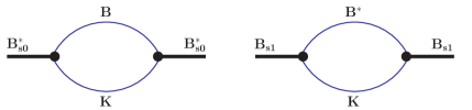
Figure 1: Mass operators of $B_{s0}^{\ast}$ and $B_{s1}$ mesons.

The mass operators of the $B_{s0}^{\ast}$ and $B_{s1}$ mesons are described by the diagrams of Fig. 1(a) and 1(b), respectively.

Following Eqs. (9a) and (9b) the coupling constants $g_{{}_{B_{s0}^{\ast}}}$ and $g_{{}_{B_{s1}}}$ can be expressed in the form:

$$\frac{1}{g_{{}_{B_{s0}^{\ast}}}^{2}} = \frac{2}{(4\pi\Lambda_{M})^{2}}\,\int\limits_{0}^{1}dx\int\limits_{0}^{\infty}\frac{d\alpha\,\alpha\,P_{0}(\alpha,x)}{(1+\alpha)^{3}}\,\,\biggl{[}-\frac{d}{dz_{0}}\tilde{\Phi}^{2}_{M}(z_{0})\biggr{]}\,,$$ (12a)

$$\frac{1}{g_{{}_{B_{s1}}}^{2}} = \frac{2}{(4\pi\Lambda_{M})^{2}}\,\int\limits_{0}^{1}dx\int\limits_{0}^{\infty}\frac{d\alpha\,\alpha\,P_{1}(\alpha,x)}{(1+\alpha)^{3}}\,\,\biggl{[}\frac{1}{2\mu_{B^{\ast}}^{2}(1+\alpha)}-\frac{d}{dz_{1}}\biggr{]}\tilde{\Phi}^{2}_{M}(z_{1})$$ (12b)

where

$$P_{0}(\alpha,x) = \alpha^{2}x(1-x)+w_{{}_{BK}}^{2}\alpha x+w_{{}_{KB}}^{2}\alpha(1-x)\,,$$

$$P_{1}(\alpha,x) = \alpha^{2}x(1-x)+w_{{}_{B^{\ast}\!K}}^{2}\alpha x+w_{{}_{KB^{\ast}}}^{2}\alpha(1-x)\,,$$ (13)

$$z_{0} = \mu_{B}^{2}\alpha x+\mu_{K}^{2}\alpha(1-x)-\frac{P_{0}(\alpha,x)}{1+\alpha}\,\mu_{B_{s0}^{\ast}}^{2}\,,$$

$$z_{1} = \mu_{B^{\ast}}^{2}\alpha x+\mu_{K}^{2}\alpha(1-x)-\frac{P_{1}(\alpha,x)}{1+\alpha}\,\mu_{B_{s1}}^{2}\,,$$

$$\mu_{M} = \frac{m_{M}}{\Lambda_{M}}\,.$$

The above expressions are valid for any functional form of the correlation function ${\widetilde{\Phi}}_{M}$.

Note that the compositeness condition of the type (9a), (9b) was originally applied to the study of the deuteron as a bound state of proton and neutron Weinberg:1962hj . Then this condition was extensively used in low-energy hadron phenomenology as the master equation for the treatment of mesons and baryons as bound states of light and heavy constituent quarks Efimov:1993ei ; Anikin:1995cf . In Refs. Baru:2003qq and Faessler:2007gv -Dong:2007px this condition was used in the application to hadronic molecule configurations of light and heavy mesons.

II.2 Effective Lagrangian for strong and radiative decays of $B_{s0}^{\ast}$ and $B_{s1}$ mesons

In Ref. Faessler:2007gv ; Faessler:2007us , in the analysis of the strong isospin-violating decays $D_{s0}^{\ast}\to D_{s}\pi^{0}$ and $D_{s1}\to D_{s}^{\ast}\pi^{0}$ in the molecular approach, we showed the existence of two possible dynamical mechanisms. This included the so-called “direct” mechanism with $\pi^{0}$-meson emission from the $D\to D^{\ast}$ and $K\to K^{\ast}$ transitions and the “indirect” mechanism where a $\pi^{0}$ meson is produced via $\eta-\pi^{0}$ mixing. The mixing is due to the mass term of pseudoscalar mesons in the leading-order $O(p^{2})$ Lagrangian of chiral perturbation theory (ChPT) Gasser:1984gg ; Cho:1994zu . Note, that the second mechanism based on $\eta-\pi^{0}$ mixing was mainly considered before in the literature. Originally it was initiated by the analysis based on the use of chiral Lagrangians Cho:1994zu ; Bardeen:2003kt ; Colangelo:2003vg ; Mehen:2004uj where the leading-order, tree-level $D_{s0}^{\ast}D_{s}\pi^{0}$ ($D_{s1}D_{s}^{\ast}\pi^{0}$) coupling can be generated only by virtual $\eta$-meson emission. In Ref. Faessler:2007us we showed that the “direct” and “mixing” mechanisms can be combined together in the form of an effective coupling of $\pi^{0}$ to the mesonic pairs $DD^{\ast}$ or $KK^{\ast}$ with modified flavor structure. This modification occurs after the diagonalization of the mesonic mass term involving $\pi^{0}$ and $\eta$ meson fields Gasser:1984gg (see details in Faessler:2007us ). In particular, instead of the $\tau_{3}\,\pi^{0}$ coupling to $DD^{\ast}$ or $KK^{\ast}$ we have $\pi^{0}\,(\tau_{3}\,\cos\varepsilon\,+\,\kappa\,I\,\sin\varepsilon)$, where $\kappa=1/\sqrt{3}$ or $\sqrt{3}$ is the corresponding flavor-algebra factor for the $DD^{\ast}$ or $KK^{\ast}$ coupling, respectively. The $\pi^{0}-\eta$ mixing angle $\varepsilon$ is fixed as Gasser:1984gg :

$$\tan 2\varepsilon=\frac{\sqrt{3}}{2}\frac{m_{d}-m_{u}}{m_{s}-\hat{m}}\simeq 0.02\,,\hskip 28.45274pt\hat{m}=\frac{1}{2}(m_{u}+m_{d})\,,$$ (14)

where $m_{u},m_{d},m_{s}$ are the current quark masses.

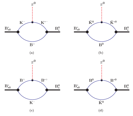
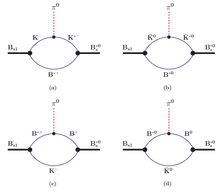
Figure 2: Diagrams contributing to the strong transition $B_{s0}^{\ast}\to B_{s}+\pi^{0}$.

Figure 3: Diagrams contributing to the strong transition $B_{s1}\to B_{s}^{\ast}+\pi^{0}$.

Below, in Eq.(17), we display the explicit form of the corresponding interaction Lagrangian. The lowest-order diagrams which contribute to the matrix elements of the strong isospin-violating decays $B_{s0}^{\ast}\to B_{s}\pi^{0}$ and $B_{s1}\to B_{s}^{\ast}\pi^{0}$ are shown in Figs.2 and 3. Note, that in the isospin limit ($m_{u}=m_{d}$), the $\eta-\pi^{0}$ mixing angle vanishes and the masses of the virtual $B^{(\ast)}$ and $K^{(\ast)}$ mesons in the loops are degenerate. As a result the pairs of diagrams related to Figs.2(a) and 2(b), Figs.2(c) and 2(d), Figs.3(a) and 3(b), Figs.3(c) and 3(d) compensate each other. Therefore, in the calculation of the diagrams of Figs.2 and 3 we go beyond the isospin limit and use the physical meson masses.

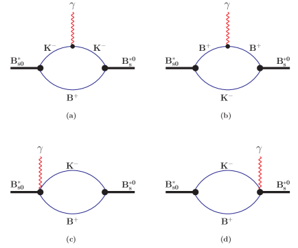
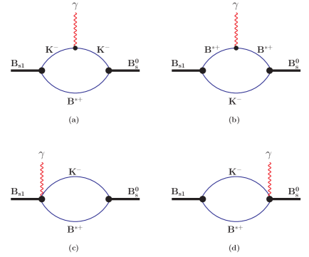
Figure 4: Diagrams contributing to the radiative transition $B_{s0}^{\ast}\to B_{s}^{\ast}+\gamma$.

Figure 5: Diagrams contributing to the radiative transition $B_{s1}\to B_{s}+\gamma$.

The diagrams contributing to the radiative decays $B_{s0}^{\ast}\to B_{s}^{\ast}\gamma$, $B_{s1}\to B_{s}\gamma$, $B_{s1}\to B_{s}^{\ast}\gamma$ and $B_{s1}\to B_{s0}^{\ast}\gamma$ are shown in Figs.4, 5, 6 and 7. The diagrams of Figs.4(a), 4(b), 5(a) and 5(b) are generated by the direct coupling of the charged $K^{-}$ and $B^{+}(B^{\ast+})$ mesons to the electromagnetic field after gauging the free Lagrangians related to these mesons. The diagrams of Figs.6(a)-6(d), 7(a) and 7(b) are generated by the coupling of a corresponding pair of vector and pseudoscalar mesons to the photon. The diagrams of Figs.4(c), 5(c), and 6(e) are generated after gauging the nonlocal strong Lagrangians (1) describing the coupling of the $B_{s0}^{\ast}$ and $B_{s1}$ mesons to their constituents. The diagrams of Figs.4(d) and 5(d) arise after gauging the strong $B_{s}^{\ast}B^{+}K^{-}$ and $B_{s}B^{\ast+}K^{-}$ interaction Lagrangian containing derivatives acting on the pseudoscalar fields. Details of how to generate the effective couplings of the involved mesons to the electromagnetic field will be discussed later.

After the preliminary discussion of the relevant diagrams, we are now in the position to write down the full effective Lagrangian for the study of the strong and radiative decays of the $B_{s0}^{\ast}$ and $B_{s1}$ mesons formulated in terms of mesonic degrees of freedom and of photons. We follow the procedure discussed in detail in Refs. Faessler:2007gv -Faessler:2007us , where we considered the $D_{s0}^{\ast}$ and $D_{s1}$ meson decay properties. First, we write the Lagrangian ${\cal L}$, which includes the free mesonic parts ${\cal L}_{\rm free}$ and the strong interaction parts ${\cal L}_{\rm str}$:

$${\cal L}(x)\,=\,{\cal L}_{\rm free}(x)\,+\,{\cal L}_{\rm str}(x)\,,$$ (15)

with

$${\cal L}_{\rm free}(x) = -\bar{B}_{s0}^{\ast\,+}(x)(\Box+m_{B_{s0}^{\ast}}^{2})B_{s0}^{\ast}(x)+\bar{B}_{s1,\mu}(x)(g^{\mu\nu}[\Box+m_{B_{s1}}^{2}]-\partial^{\mu}\partial^{\nu})B_{s1,\nu}(x)$$ (16)

$$- \frac{1}{2}\vec{\pi}(x)(\Box+m_{\pi}^{2})\vec{\pi}(x)+\frac{\delta_{\pi}}{2}\,[\pi^{0}(x)]^{2}-\sum\limits_{P=K,B,B_{s}}P^{\dagger}(x)(\Box+m_{P}^{2})P(x)+\sum\limits_{P=K,B}\delta_{P}\,\bar{P}^{0}(x)P^{0}(x)$$

$$+ \sum\limits_{V=K^{\ast},B^{\ast},B_{s}^{\ast}}V^{\dagger}_{\mu}(x)(g^{\mu\nu}[\Box+m_{V}^{2}]-\partial^{\mu}\partial^{\nu})V_{\nu}(x)-\sum\limits_{V=K^{\ast},B^{\ast}}\delta_{V}\,\bar{V}^{0}_{\mu}(x)V^{0\,\mu}(x)\,,$$

$${\cal L}_{\rm str}(x) = \frac{g_{{}_{B^{\ast}B\pi}}}{2\sqrt{2}}\,B^{\ast\,\dagger}_{\mu}(x)\,\hat{\pi}_{B}(x)\,i\!\stackrel{{\scriptstyle\leftrightarrow}}{{\partial}}^{\,\mu}\!\!B(x)+\frac{g_{{}_{K^{\ast}K\pi}}}{\sqrt{2}}\,K^{\ast\,\dagger}_{\mu}(x)\,\hat{\pi}_{K}(x)\,i\!\stackrel{{\scriptstyle\leftrightarrow}}{{\partial}}^{\,\mu}\!\!K(x)$$ (17)

$$+ g_{{}_{B_{s}B^{\ast}K}}\,B^{\ast\,\dagger}_{\mu}(x)\,K(x)\,i\!\stackrel{{\scriptstyle\leftrightarrow}}{{\partial}}^{\,\mu}\!\!B_{s}^{0}(x)+g_{{}_{B_{s}BK^{\ast}}}\,K^{\ast\,\dagger}_{\mu}(x)\,B(x)\,i\!\stackrel{{\scriptstyle\leftrightarrow}}{{\partial}}^{\,\mu}\!\!\bar{B}_{s}^{0}(x)+g_{{}_{B^{\ast}_{s}BK}}B^{\ast\,0}_{s,\mu}(x)\,B^{\dagger}(x)\,i\!\stackrel{{\scriptstyle\leftrightarrow}}{{\partial}}^{\,\mu}\!\!K(x)$$

$$- ig_{{}_{B_{s}^{\ast}B^{\ast}K^{\ast}}}\,\biggl{[}B^{\ast\,0\,\mu\nu}_{s}(x)B^{\ast\,\dagger}_{\mu}(x)K^{\ast}_{\nu}(x)+B^{\ast\,\dagger}_{\mu\nu}(x)K^{\ast\,\mu}(x)B^{\ast\,0\,\nu}_{s}(x)+K^{\ast\,\mu\nu}(x)B^{\ast\,0}_{s,\mu}(x)B^{\ast\,\dagger}_{\nu}(x)\biggr{]}$$

$$+ \frac{g_{B_{s}^{\ast}B^{\ast}K}}{4}\epsilon^{\mu\nu\alpha\beta}B^{\ast}_{s\,\mu\nu}(x)B^{\ast\,\dagger}_{\alpha\beta}(x)K(x)+{\cal L}_{B_{s0}^{\ast}}(x)+{\cal L}_{B_{s1}}(x)\,+\,{\rm H.c.}\,,$$

where summation over isospin indices is understood, $\Box=\partial^{\mu}\partial_{\mu}$ and $A\stackrel{{\scriptstyle\leftrightarrow}}{{\partial}}B\equiv A\partial B-B\partial A$. Here, $\vec{\pi}=(\pi_{1},\pi_{2},\pi_{3})$ is the triplet of pions, $\hat{\pi}_{B}=\pi_{1}\tau_{1}+\pi_{2}\tau_{2}+\pi_{3}(\tau_{3}\cos\varepsilon+I\sin\varepsilon/\sqrt{3})$, $\hat{\pi}_{K}=\pi_{1}\tau_{1}+\pi_{2}\tau_{2}+\pi_{3}(\tau_{3}\cos\varepsilon+I\sin\varepsilon\sqrt{3})$, $B^{(\ast)}$ and $K^{(\ast)}$ are the doublets of pseudoscalar (vector) mesons, $B_{s}^{\pm}$ and $B_{s}^{\ast\,\pm}$ are the pseudoscalar and vector bottom-strange mesons, respectively, $V^{\ast\,\mu\nu}=\partial^{\mu}V^{\ast\,\nu}-\partial^{\nu}V^{\ast\,\mu}$ is the stress tensor of the vector meson field.

In our convention the isospin-symmetric meson masses of the isomultiplets $m_{\pi},m_{P},m_{V}$ are identified with the masses of the charged partners. The quantities $\delta_{M}$ are the isospin-breaking parameters which are fixed by the difference of masses squared of the charged and neutral members of the isomultiplets as: $\delta_{M}=m_{M^{\pm}}^{2}-m_{M^{0}}^{2}$ and $m_{M^{0}}\equiv m_{\bar{M}^{0}}\,.$ The set of mesonic masses is taken from data Yao:2006px . From Eq. (17) it is evident that the couplings of $\pi^{0}$ to the $B^{\ast}B$ and $K^{\ast}K$ mesonic pairs contain two terms — the “dominant” coupling (proportional to $\cos\varepsilon$) and the “suppressed” coupling (proportional to $\sin\varepsilon$). This means that the first coupling survives in the isospin limit, while the second one vanishes.

The free meson propagators are given by the standard expressions

$$i\,D_{M}(x-y)=\langle 0|T\,M(x)\,M^{\dagger}(y)|0\rangle\ =\ \int\frac{d^{4}k}{(2\pi)^{4}i}\,e^{-ik(x-y)}\ \tilde{D}_{M}(k)$$ (18)

for the scalar (pseudoscalar) fields, where $\tilde{D}_{M}(k)=(m_{M}^{2}-k^{2}-i\epsilon)^{-1}$ and

$$i\,D_{M^{\ast}}^{\mu\nu}(x-y)=\langle 0|T\,M^{\ast\,\mu}(x)\,M^{\ast\,\nu\,\dagger}(y)|0\rangle\ =\ \int\frac{d^{4}k}{(2\pi)^{4}i}\,e^{-ik(x-y)}\ \tilde{D}_{M^{\ast}}^{\mu\nu}(k)$$ (19)

for the vector (axial) fields, where $\tilde{D}_{M^{\ast}}^{\mu\nu}(k)=(-g^{\mu\nu}+k^{\mu}k^{\nu}/m_{M^{\ast}}^{2})\,(m_{M^{\ast}}^{2}-k^{2}-i\epsilon)^{-1}\,.$ The choice for the strong meson couplings of the Lagrangian (17) will be discussed in Sec.III.

The electromagnetic field is included in the Lagrangian (15) using minimal substitution i.e. each derivative acting on a charged meson field is replaced by the covariant one: $\partial^{\mu}M^{(\ast)\pm}\,\to\,(\partial^{\mu}\mp ieA^{\mu})\,M^{(\ast)\pm}\,.$ Note, that the strong interaction Lagrangians ${\cal L}_{B_{s0}^{\ast}}$ and ${\cal L}_{B_{s1}}$ should also be modified in order to restore electromagnetic gauge invariance. It proceeds in a way as suggested in Ref. Mandelstam:1962mi and is extensively used in Refs. Anikin:1995cf ; Faessler:2007gv ; Faessler:2007us . In particular, each charged constituent meson field $H^{\pm}$ (i.e. $B^{(\ast\pm)}$ and $K^{(\pm)}$) in ${\cal L}_{B_{s0}^{\ast}}$ and ${\cal L}_{B_{s1}}$ is multiplied by the gauge field exponential (see further details in Anikin:1995cf ; Faessler:2007gv ; Faessler:2007us ):

$$H^{\pm}(y)\to e^{\mp ieI(y,x,P)}H^{\pm}(y)$$ (20)

where

$$I(x,y,P)=\int\limits_{y}^{x}dz_{\mu}A^{\mu}(z).$$ (21)

For the derivative of $I(x,y,P)$ we use the path-independent prescription suggested in Mandelstam:1962mi which in turn states that the derivative of $I(x,y,P)$ does not depend on the path $P$ originally used in the definition. The nonminimal substitution (20) is therefore completely equivalent to the minimal prescription. Expanding the exponential $e^{\mp ieI(y,x,P)}H^{\pm}(y)$ in powers of the electromagnetic field and keeping linear terms like the four-particle coupling $B_{s0}^{\ast}B^{+}K^{-}\gamma$ and $B_{s1}B^{\ast+}K^{-}\gamma$ we generate the diagrams of Figs.4(c) and 5(c), 6(c), 6(d), respectively.

Finally, we specify the electromagnetic Lagrangian describing the coupling of vector and pseudoscalar mesons to the photon:

$${\cal L}_{VP\gamma}(x) = \frac{e}{4}\,F_{\mu\nu}(x)\,\epsilon^{\mu\nu\alpha\beta}\biggl{(}g_{{}_{K^{\ast\,\pm}K^{\pm}\gamma}}\,K^{\ast\,+}_{\alpha\beta}(x)\,K^{-}(x)+g_{{}_{K^{\ast\,0}K^{0}\gamma}}\,K^{\ast\,0}_{\alpha\beta}(x)\,\bar{K}^{0}(x)$$ (22)

$$+ g_{{}_{B^{\ast\,\pm}B^{\pm}\gamma}}\,B^{\ast\,+}_{\alpha\beta}(x)\,B^{-}(x)+g_{{}_{B^{\ast\,0}B^{0}\gamma}}\,B^{\ast\,0}_{\alpha\beta}(x)\,\bar{B}^{0}(x)\biggr{)}\,+\,{\rm H.c.}$$

Here the couplings $g_{{}_{VP\gamma}}$ can be extracted from the corresponding decay widths $V\to P+\gamma$. Presently we only have information about the decay width of $K^{\ast}$ mesons. Using the expressions for the $K^{\ast}\to K+\gamma$ decay widths

$$\Gamma(K^{\ast}\to K\gamma)=\frac{\alpha}{24}\,g_{{}_{K^{\ast}K^{\gamma}}}^{2}\,m_{K^{\ast}}^{3}\,\biggl{(}1-\frac{m_{K}^{2}}{m_{K^{\ast}}^{2}}\biggr{)}^{3}\,$$ (23)

and the data (central values) for $\Gamma(K^{\ast\,\pm}\to K^{\pm}\gamma)=50.29$ keV and $\Gamma(K^{\ast\,0}\to K^{0}\gamma)=116.19$ keV we deduce the coupling constants $g_{{}_{K^{\ast\,\pm}\to K^{\pm}\gamma}}=0.836$ GeV^-1 and $g_{{}_{K^{\ast\,0}\to K^{0}\gamma}}=-1.267$ GeV^-1. Note, that in the nonrelativistic SU(3) quark model the couplings $g_{{}_{K^{\ast\,\pm}\to K^{\pm}\gamma}}$ and $g_{{}_{K^{\ast\,0}\to K^{0}\gamma}}$ are proportional to the sum of the charges of the constituent quarks: $g_{{}_{K^{\ast\,\pm}\to K^{\pm}\gamma}}\sim(e_{u}+e_{s})=1/3$ and $g_{{}_{K^{\ast\,0}\to K^{0}\gamma}}\sim(e_{d}+e_{s})=-2/3$. This is the reason why the coupling of the neutral kaons is defined (by convention) with a negative sign. Also, the prediction of the nonrelativistic quark model for the ratio $g_{{}_{K^{\ast\,0}\to K^{0}\gamma}}/g_{{}_{K^{\ast\,\pm}\to K^{\pm}\gamma}}=-2$ is violated by relativistic corrections. For $D$ mesons the corresponding ratio is in precise agreement with data. In particular, taking the experimental values of $g_{{}_{D^{\ast\,\pm}\to D^{\pm}\gamma}}\simeq 0.5$ GeV^-1 and $g_{{}_{D^{\ast\,\pm}\to D^{\pm}\gamma}}\simeq 2.0$ GeV^-1 (see the discussion in Ref. Dong:2008gb ) we get

$$\frac{g_{{}_{D^{\ast\,0}\to D^{0}\gamma}}}{g_{{}_{D^{\ast\,\pm}\to D^{\pm}\gamma}}}=\frac{e_{c}+e_{u}}{e_{c}+e_{d}}=4\,.$$ (24)

Therefore, one can expect that for bottom mesons the naive quark model should prediction should also be sufficient:

$$\frac{g_{{}_{B^{\ast\,0}\to B^{0}\gamma}}}{g_{{}_{B^{\ast\,\pm}\to B^{\pm}\gamma}}}=\frac{e_{b}+e_{d}}{e_{b}+e_{u}}=-2\,.$$ (25)

For our numerical estimates we will use typical values with $g_{{}_{B^{\ast\,\pm}\to B^{\pm}\gamma}}=0.5$ GeV^-1 and $g_{{}_{B^{\ast\,0}\to B^{0}\gamma}}=-1$ GeV^-1. These couplings correspond to the full width of $B^{\ast\,\pm}$ equal to 0.23 keV and and of $B^{\ast\,0}$ equal to 0.91 keV (as usual we suppose that $B^{\ast}\to B\gamma$ is the dominant mode for the $B^{\ast}$ mesons).

III Strong and radiative decays of the $B_{s0}^{\ast}$ and $B_{s1}$ mesons

III.1 Matrix elements and decay widths

The matrix elements describing the strong $B_{s0}^{\ast}\to B_{s}\pi^{0}$, $B_{s1}\to B_{s}^{\ast}\pi^{0}$ and radiative $B_{s0}^{\ast}\to B_{s}^{\ast}\gamma$, $B_{s1}\to B_{s}\gamma$ decays are defined as follows

$$M(B_{s0}^{\ast}(p)\to B_{s}(p^{\prime})\pi^{0}(q)) = G_{B_{s0}^{\ast}B_{s}\pi}\,,$$ (26a)

$$M(B_{s1}(p)\to B_{s}^{\ast}(p^{\prime})\pi^{0}(q)) = \epsilon_{\mu}(p)\epsilon^{\ast}_{\nu}(p^{\prime})\ (g^{\mu\nu}\ G_{B_{s1}B_{s}^{\ast}\pi}\ -\ v^{\prime\mu}v^{\nu}\ F_{B_{s1}B_{s}^{\ast}\pi})\,,$$ (26b)

and

$$M(B_{s0}^{\ast}(p)\to B_{s}^{\ast}(p^{\prime})\gamma(q)) = e\ \epsilon_{\mu}^{\ast}(q)\epsilon_{\nu}^{\ast}(p^{\prime})\,(g_{\mu\nu}p^{\prime}q-p^{\prime}_{\mu}q_{\nu})\ G_{B_{s0}^{\ast}B_{s}^{\ast}\gamma}\,,$$ (27a)

$$M(B_{s1}(p)\to B_{s}(p^{\prime})\gamma(q)) = e\ \epsilon_{\mu}(p)\epsilon^{\ast}_{\nu}(q)\ (g^{\mu\nu}\ pq\ -\ q^{\mu}p^{\nu})\ G_{B_{s1}B_{s}\gamma}\,,$$ (27b)

$$M(B_{s1}(p)\to B_{s}^{\ast}(p^{\prime})\gamma(q)) = e\,\varepsilon^{mn\rho\sigma}\,\epsilon^{\alpha}(p)\,\epsilon^{\ast\mu}(p^{\prime})\,\epsilon_{\rho}^{\ast}(q)\,q_{\sigma}\,\biggl{(}G_{B_{s1}B_{s}^{\ast}\gamma}\,g_{\mu n}g_{\alpha m}\,pq$$ (27c)

$$+ \,F_{B_{s1}B_{s}^{\ast}\gamma}\,g_{\mu n}\,p_{m}q_{\alpha}\,+\,H_{B_{s1}B_{s}^{\ast}\gamma}\,g_{\alpha m}\,p_{n}q_{\mu}\biggr{)}\,,$$

$$M(B_{s1}(p)\to B_{s0}^{\ast}(p^{\prime})\gamma(q)) = e\ \varepsilon^{\mu\nu\alpha\beta}\ \epsilon_{\mu}(p)\epsilon^{\ast}_{\nu}(q)\ p_{\alpha}\ q_{\beta}\ G_{B_{s1}B_{s0}\gamma}\,,$$ (27d)

where $v=p/m_{B_{s1}}$ and $v^{\prime}=p^{\prime}/m_{B_{s}^{\ast}}$ are the four-velocities of the $B_{s1}$ and $B_{s}^{\ast}$ mesons, $G_{B_{s0}^{\ast}B_{s}\pi}$, $G(F)_{B_{s1}B_{s}^{\ast}\pi}$, $G_{B_{s0}^{\ast}B_{s}^{\ast}\gamma}$ and $G_{B_{s1}B_{s}\gamma}$, $G(F,H)_{B_{s1}B_{s}^{\ast}\gamma}$ and $G_{B_{s1}B_{s0}^{\ast}\gamma}$ are the corresponding effective coupling constants. The coherent sum of all the diagrams in Figs.4-7, contributing to the radiative decays of $B_{s0}^{\ast}$ and $B_{s1}$ mesons, is gauge invariant, while the contribution of each diagram is definitely not gauge invariant. As done in Ref. Faessler:2007gv , for convenience we split each individual diagram into a gauge-invariant piece and a remainder, which is noninvariant. One can prove that the sum of the noninvariant terms vanishes due to gauge invariance. In the following discussion of the numerical results we will only deal with the gauge-invariant contribution of the separate diagrams of Figs.4-7. In Appendix A we present the calculational technique for determining the effective couplings entering in the matrix elements of the strong and radiative transitions of $B_{s0}^{\ast}$ and $B_{s1}$ mesons.

Using Eqs. (26) and (27) the strong $B_{s0}^{\ast}\to B_{s}\pi^{0}$, $B_{s1}\to B_{s}^{\ast}\pi^{0}$ and radiative $B_{s0}^{\ast}\to B_{s}^{\ast}\gamma$, $B_{s1}\to B_{s}\gamma$, $B_{s1}\to B_{s}^{\ast}\gamma$, $B_{s1}\to B_{s0}^{\ast}\gamma$ decay widths are calculated according to the expressions:

$$\Gamma(B_{s0}^{\ast}\to B_{s}\pi^{0})\, = \,\frac{G_{B_{s0}^{\ast}B_{s}\pi}^{2}}{8\pi m_{B_{s0}^{\ast}}^{2}}\,P_{\pi 1}\,,$$ (28a)

$$\Gamma(B_{s1}\to B_{s}^{\ast}\pi^{0}) = \frac{P_{\pi 2}}{12\pi m_{B_{s1}}^{2}}\,\biggl{\{}G_{B_{s1}B_{s}^{\ast}\pi}^{2}+\frac{1}{2}\biggl{(}G_{B_{s1}B_{s}^{\ast}\pi}\,w-F_{B_{s1}B_{s}^{\ast}\pi}(w^{2}-1)\biggr{)}^{2}\biggr{\}}\,,$$ (28b)

and

$$\Gamma(B_{s0}^{\ast}\to B_{s}^{\ast}\gamma) = \alpha\,G_{B_{s0}^{\ast}B_{s}^{\ast}\gamma}^{2}\,P_{\gamma 1}^{3}\,,$$ (29a)

$$\Gamma(B_{s1}\to B_{s}\gamma) = \frac{\alpha}{3}\,G_{B_{s1}B_{s}\gamma}^{2}\,P_{\gamma 2}^{3}\,,$$ (29b)

$$\Gamma(B_{s1}\to B_{s}^{\ast}\gamma) = \frac{\alpha}{3}\,P_{\gamma 3}^{5}\,\biggl{\{}\biggl{(}G_{B_{s1}B_{s}^{\ast}\gamma}+F_{B_{s1}B_{s}^{\ast}\gamma}\biggr{)}^{2}+\frac{m_{B_{s1}}^{2}}{m_{B_{s}^{\ast}}^{2}}\biggl{(}G_{B_{s1}B_{s}^{\ast}\gamma}+H_{B_{s1}B_{s}^{\ast}\gamma}\biggr{)}^{2}\biggr{\}}\,,$$ (29c)

$$\Gamma(B_{s1}\to B_{s0}^{\ast}\gamma) = \frac{\alpha}{3}\,G_{B_{s1}B_{s0}^{\ast}\gamma}^{2}\,P_{\gamma 4}^{3}\,,$$ (29d)

where $w=vv^{\prime}=(m_{B_{s1}}^{2}+m_{B_{s}^{\ast}}^{2}-m_{\pi^{0}}^{2})/(2m_{B_{s1}}m_{B_{s}^{\ast}})$ and $P_{\pi i}$, $P_{\gamma i}$ are the corresponding three-momenta of the decay products.

Note, the contribution of the effective coupling constant $F_{B_{s1}B_{s}^{\ast}\pi}$ to the $B_{s1}\to B_{s}^{\ast}\pi^{0}$ decay width is strongly suppressed. This is because the contribution of the matrix element with $F_{B_{s1}B_{s}^{\ast}\pi}$ is proportional to the suppressed factor $w^{2}-1\simeq 4\times 10^{-3}$ with $w\simeq 1$. Therefore, we have

$$\Gamma(B_{s1}\to B_{s}^{\ast}\pi^{0})\ \simeq\ \frac{G_{B_{s1}B_{s}^{\ast}\pi}^{2}}{8\pi m_{B_{s1}}^{2}}\,P_{\pi 2}\,$$ (30)

and

$$\frac{\Gamma(B_{s1}\to B_{s}^{\ast}\pi^{0})}{\Gamma(B_{s0}^{\ast}\to B_{s}\pi^{0})}\ \simeq\ \frac{P_{\pi 2}}{P_{\pi 1}}\,\biggl{(}\frac{m_{B_{s0}^{\ast}}}{m_{B_{s1}}}\biggr{)}^{2}\,\biggl{(}\frac{G_{B_{s1}B_{s}^{\ast}\pi}}{G_{B_{s0}^{\ast}B_{s}\pi}}\biggr{)}^{2}\,.$$ (31)

III.2 Numerical results

First, we discuss the choice for the strong coupling constants in the Lagrangian ${\cal L}_{\rm str}$ (15). In Refs. Faessler:2007gv ; Faessler:2007us we used the set of strong coupling constants $g_{{}_{D_{1}D_{2}L}}$ $(g_{{}_{D^{\ast}D\pi}}$, $g_{{}_{D_{s}D^{\ast}K}}=g_{{}_{D_{s}K^{\ast}D}}$ and $g_{{}_{D_{s}^{\ast}DK}}=g_{{}_{D_{s}^{\ast}D^{\ast}K^{\ast}}})$ defined in the charm sector, where index $L$ denotes a light meson, while $D_{1}$ and $D_{2}$ are the respective charm states. The coupling $g_{{}_{D^{\ast}D\pi}}=17.9$ was deduced using data for the corresponding strong decay width Anastassov:2001cw . The coupling constants $g_{{}_{D_{s}D^{\ast}K}}$ and $g_{{}_{D_{s}^{\ast}DK}}$ have been estimated using two different variants of the QCD sum rule approach discussed in Refs. Wang:2006id ; Bracco:2006xf , where similar results have been obtained. Both Refs. Wang:2006id ; Bracco:2006xf point to a strong suppression of these constants in comparison to the coupling $g_{{}_{D^{\ast}D\pi}}$. An updated analysis for $g_{{}_{D^{\ast}D\pi}}$ in the context of a QCD sum rule approach gives a result close to data – $g_{{}_{D^{\ast}D\pi}}=14\pm 1.5$ Navarra:2001ju . We used the predictions of Ref. Wang:2006id : $g_{{}_{D^{\ast}D_{s}K}}=2.02$ and $g_{{}_{D_{s}^{\ast}DK}}=1.84$. For the unknown parameters $g_{{}_{D_{s}K^{\ast}D}}$ and $g_{{}_{D_{s}^{\ast}D^{\ast}K^{\ast}}}$ we used the approximative relations $g_{{}_{D_{s}K^{\ast}D}}\simeq g_{{}_{D_{s}D^{\ast}K}}$ and $g_{{}_{D_{s}^{\ast}D^{\ast}K^{\ast}}}\simeq g_{{}_{D_{s}^{\ast}DK}}$, which can be explained phenomenologically: the first relation – by the universality of the coupling of the $D_{s}$ meson to $D^{\ast}K$ and $K^{\ast}D$ mesonic pairs (it is based on exact SU(4) flavor symmetry and we do not expect a substantial violation of this relation due to breaking of the SU(4) symmetry) and the second relation – by the universality of the coupling of the $D_{s}^{\ast}$ meson to two pseudoscalars and two vectors (like for $\rho\pi\pi$ and $\rho\rho\rho$ couplings: $g_{\rho\pi\pi}\simeq g_{\rho\rho\rho}\simeq 6$, and also for $J/\Psi DD$ and $J\Psi D^{\ast}D^{\ast}$: $g_{J/\Psi DD}\simeq g_{J/\Psi D^{\ast}D^{\ast}}\simeq 8$ Lin:1999ad ). For consistency, in the present manuscript we use the set of charmed hadronic couplings predicted by QCD sum rules (central values) with :

$$g_{{}_{D^{\ast}D\pi}}=14\,,\hskip 14.22636ptg_{{}_{D_{s}D^{\ast}K}}=g_{{}_{D_{s}K^{\ast}D}}=2.02\,,\hskip 14.22636ptg_{{}_{D_{s}^{\ast}DK}}=g_{{}_{D_{s}^{\ast}D^{\ast}K^{\ast}}}=1.84\,.$$ (32)

In particular, instead of $g_{{}_{D^{\ast}D\pi}}=17.9$ we use $g_{{}_{D^{\ast}D\pi}}=14$. Such a modification does not change the numerical results of Refs. Faessler:2007gv ; Faessler:2007us , because the contribution of the corresponding diagrams containing the coupling $g_{{}_{D^{\ast}D\pi}}$ is strongly suppressed. A similar picture we also have in the bottom sector (see discussion below).

In order to evaluate the corresponding bottom couplings $g_{{}_{B_{1}B_{2}L}}$ we use the arguments of heavy hadron chiral perturbation theory (HHChPT) Wise:1992hn ; Casalbuoni:1996pg which relates the bottom and charmed couplings containing the same light meson:

$$g_{{}_{B_{1}B_{2}L}}=g_{{}_{D_{1}D_{2}L}}\,\displaystyle\frac{m_{B}}{m_{D}}$$ (33)

where $m_{B}$ and $m_{D}$ are the masses of the bottom and charm mesons identified e.g. with the masses of $m_{B^{\pm}}=5.279$ GeV and $m_{D^{\pm}}=1.8693$ GeV. In other words, to get the set of bottom meson couplings used in the strong Lagrangian (17) we rescale the corresponding charm meson couplings by a factor $m_{B^{\pm}}/m_{D^{\pm}}\simeq 2.82$. In particular, we have:

$$g_{{}_{B^{\ast}B\pi}}=39.5\,,\hskip 14.22636ptg_{{}_{B_{s}B^{\ast}K}}\simeq g_{{}_{B_{s}K^{\ast}B}}=5.70\,,\hskip 14.22636ptg_{{}_{B_{s}^{\ast}BK}}\simeq g_{{}_{B_{s}^{\ast}B^{\ast}K^{\ast}}}=5.19\,.$$ (34)

For the coupling $g_{B_{s}^{\ast}B^{\ast}K}$ we have no further input. From a dimensional analysis it should be of order 1 GeV^-1. The diagrams 6(e) and 6(f), however, where this coupling enters, are strongly suppressed, and we therefore do not need to have precise knowledge of this constant.

The coupling $g_{{}_{K^{\ast}K\pi}}=4.61$ is fixed from data on the $K^{\ast}K\pi$ decay width Yao:2006px . Finally, we fix the couplings $g_{{}_{B_{s0}^{\ast}}}$ and $g_{{}_{B_{s1}}}$, which are given by Eqs. (12a) and (12b) in terms of the adjustable vertex function. Using the Gaussian vertex function we obtain the result that these couplings are quite stable with respect to a variation of the scale parameter $\Lambda_{M}$. In particular, varying $\Lambda_{M}$ from 1 to 2 GeV, we get a range of values for $g_{{}_{B_{s0}^{\ast}}}$ from 27.17 to 23.21 GeV and for $g_{{}_{B_{s1}}}$ from 25.64 to 22.14 GeV. Note that our predictions for these couplings are in agreement with the results of other theoretical approaches: $g_{{}_{B_{s0}^{\ast}}}=g_{{}_{B_{s1}}}=19.6\pm 5.7$ GeV [light–cone QCD sum rules approach Wang:2008tm ] and $g_{{}_{B_{s0}^{\ast}}}=23.572$ GeV and $g_{{}_{B_{s1}}}=23.442$ GeV [effective chiral approach Guo:2006fu ; Guo:2006rp ].

Now we present the numerical results. First, we discuss the results for strong decays. Here the main contribution to the decay width comes, as expected, from the diagrams of Figs.2(a), (b) and 3(a), (b). On the other hand, the contribution of the direct mechanism is comparable to the one of the indirect mechanism (i.e. due to $\eta-\pi^{0}$ mixing). The contribution of the diagrams in Figs.2(c) and (d) is of order 0.1% of the total contribution to the $G_{B_{s0}^{\ast}B_{s}\pi}$ coupling and the contribution of Figs.3(c) and (d) is of order 1.6% of the total contribution to the $G_{B_{s1}B_{s}^{\ast}\pi}$ coupling. Therefore, the couplings $G_{B_{s0}^{\ast}B_{s}\pi}$ and $G_{B_{s1}B_{s}^{\ast}\pi}$ are not sensitive to a variation of the couplings $g_{{}_{B^{\ast}B\pi}}$, $g_{{}_{B_{s}^{\ast}BK}}$ and $g_{{}_{B_{s}B^{\ast}K}}$. They are only sensitive to the values of the couplings $g_{{}_{B_{s}K^{\ast}B}}$ and $g_{{}_{B_{s}^{\ast}B^{\ast}K^{\ast}}}$. The leading-order contributions from the diagrams in Figs.2(a), (b) and 3(a), (b) to the quantities $G_{B_{s0}^{\ast}B_{s}\pi}$ and $G_{B_{s1}B_{s}^{\ast}\pi}$ in terms of the couplings $g_{{}_{B_{s}K^{\ast}B}}$ and $g_{{}_{B_{s}^{\ast}B^{\ast}K^{\ast}}}$ are given by

$$G_{B_{s0}^{\ast}B_{s}\pi}=65.9\ g_{{}_{B_{s}K^{\ast}B}}\ {\rm MeV}\,,\hskip 14.22636ptG_{B_{s1}B_{s}^{\ast}\pi}=72.3\ g_{{}_{B_{s}^{\ast}B^{\ast}K^{\ast}}}\ {\rm MeV}$$ (35)

for a typical value of the dimensional parameter $\Lambda_{M}=1$ GeV. Then, using the specific values of $g_{{}_{B_{s}K^{\ast}B}}=5.70$ and $g_{{}_{B_{s}^{\ast}B^{\ast}K^{\ast}}}=5.19$ we get the following predictions for the effective couplings and decay widths:

$$G_{B_{s0}^{\ast}B_{s}\pi}=375.7(375.6)\ {\rm MeV}\,,\hskip 14.22636ptG_{B_{s1}B_{s}^{\ast}\pi}=381.1(376.3)\ {\rm MeV}$$ (36)

and

$$\Gamma(B_{s0}^{\ast}\to B_{s}\pi^{0})=55.2(55.1)\ {\rm keV}\,,\hskip 14.22636pt\Gamma(B_{s1}\to B_{s}^{\ast}\pi^{0})=57.0(55.6)\ {\rm keV}\,.$$ (37)

In the brackets we indicate the results of the leading diagrams of Figs.2(a), (b) and 3(a), (b).

The strong decay couplings $G_{B_{s0}^{\ast}B_{s}\pi}$, $G_{B_{s1}B_{s}^{\ast}\pi}$ and the decay widths $\Gamma(B_{s0}^{\ast}\to B_{s}\pi)$, $\Gamma(B_{s1}\to B_{s}^{\ast}\pi)$ are practically degenerate, which can also be explained by heavy quark symmetry (HQS), which is a good symmetry for the heavy-light mesons with a bottom quark. Because of the infinitely heavy mass of the bottom quark the spins of the $\bar{b}$ antiquark and the $s$ quark decouple (spin symmetry), and, therefore, the properties of $B_{s0}^{\ast}$ and $B_{s1}$ mesons become similar. This issue was also discussed in Refs. Colangelo:2003vg ; Mehen:2004uj in the context of the charm partners ($D_{s0}^{\ast}$ and $D_{s1}$). In particular, it was shown that the corresponding coupling constants and widths are degenerate in the heavy quark limit. In our previous papers we also reproduced the same result. Moreover, for finite charmed meson masses the decay characteristics are nearly degenerate:

$$G_{D_{s0}^{\ast}D_{s}\pi}=145.4\ {\rm MeV}\,,\hskip 14.22636ptG_{D_{s1}D_{s}^{\ast}\pi}=160.2\ {\rm MeV}$$ (38)

and

$$\Gamma(D_{s0}^{\ast}\to D_{s}\pi^{0})=46.7\ {\rm keV}\,,\hskip 14.22636pt\Gamma(D_{s1}\to D_{s}^{\ast}\pi^{0})=50.1\ {\rm keV}\,.$$ (39)

The next point is a check of the flavor content of HQS. In our molecular approach the leading contributions to the couplings $G_{H_{s0}^{\ast}H_{s}\pi}$ and $G_{H_{s1}H_{s}^{\ast}\pi}$, where $H=D$ or $B$, are defined by the pairs of diagrams in Figs.2(a,b) and 3(a,b), respectively:

$$G_{H_{s0}^{\ast}H_{s}\pi} = g_{{}_{H_{s0}^{\ast}}}\,g_{{}_{K^{\ast}K\pi}}\,g_{{}_{H_{s}HK^{\ast}}}\,I_{KK^{\ast}H}\,,$$ (40a)

$$G_{H_{s1}H_{s}^{\ast}\pi} = g_{{}_{H_{s1}}}\,g_{{}_{K^{\ast}K\pi}}\,g_{{}_{H_{s}^{\ast}H^{\ast}K^{\ast}}}\,I_{KK^{\ast}H^{\ast}}\,,$$ (40b)

where $I_{KK^{\ast}H}$ and $I_{KK^{\ast}H^{\ast}}$ are the structure integrals which are of order $O(1/m_{Q})$ in the inverse heavy quark mass expansion – $1/m_{Q}$. The hadronic couplings scale as:

$$g_{{}_{H_{s0}^{\ast}}}\sim O(m_{Q})\,,\hskip 7.11317ptg_{{}_{H_{s1}}}\sim O(m_{Q})\,,\hskip 7.11317ptg_{{}_{K^{\ast}K\pi}}\sim O(1)\,,\hskip 7.11317ptg_{{}_{H_{s}HK^{\ast}}}\sim O(m_{Q})\,,\hskip 7.11317ptg_{{}_{H_{s}^{\ast}H^{\ast}K^{\ast}}}\sim O(m_{Q})\,.$$ (41)

Therefore, the strong couplings $G_{H_{s0}^{\ast}H_{s}\pi}$ and $G_{H_{s1}H_{s}^{\ast}\pi}$ scale as: $G_{H_{s0}^{\ast}H_{s}\pi}\sim O(m_{Q})$ and $G_{H_{s1}H_{s}^{\ast}\pi}\sim O(m_{Q}).$ For this scaling behavior the following relations result:

$$\frac{G_{B_{s0}^{\ast}B_{s}\pi}}{G_{D_{s0}^{\ast}D_{s}\pi}}\sim\frac{m_{b}}{m_{c}}\,,\hskip 14.22636pt\frac{G_{B_{s1}B_{s}^{\ast}\pi}}{G_{D_{s1}D_{s}^{\ast}\pi}}\sim\frac{m_{b}}{m_{c}}\,.$$ (42)

With our results [see Eqs. (36) and (38)] we conclude that the constraints (42) are fulfilled very well.

In Table 1 we present our results for the decay widths $\Gamma(B_{s0}^{\ast}\to B_{s}\pi^{0})$ and $\Gamma(B_{s1}\to B_{s}^{\ast}\pi^{0})$ including a variation of the scale parameter $\Lambda_{M}$ from $1$ to $2$ GeV (an increase of $\Lambda_{M}$ leads to an increase of the widths) and compare them with known theoretical predictions Bardeen:2003kt ; Guo:2006fu ; Guo:2006rp ; Wang:2008ny . Our results for the decay widths are larger in comparison to previous approaches Bardeen:2003kt ; Guo:2006fu ; Guo:2006rp ; Wang:2008ny due to inclusion of the direct isospin-violating transitions $B_{s0}^{\ast}\to B_{s}\pi^{0}$ and $B_{s1}\to B_{s}^{\ast}\pi^{0}$.

Now we turn to the discussion of the radiative decays $B_{s0}^{\ast}\to B_{s}^{\ast}\gamma$ and $B_{s1}\to B_{s}\gamma$. The main contribution to the decay characteristics of the $B_{s0}^{\ast}\to B_{s}^{\ast}\gamma$ and $B_{s1}\to B_{s}\gamma$ decays comes, as expected, from the diagrams of Figs.4(a) and 5(a). Our results for the effective coupling constants and decay widths for a typical value of $\Lambda_{M}=1$ GeV are:

$$G_{B_{s0}^{\ast}B_{s}^{\ast}\gamma}\ =\ 0.122\ {\rm GeV}^{-1}\,,\hskip 14.22636ptG_{B_{s1}B_{s}\gamma}\ =\ 0.115\ {\rm GeV}^{-1}$$ (43)

and

$$\Gamma(B_{s0}^{\ast}\to B_{s}^{\ast}\gamma)\ =\ 3.07\ {\rm keV}\,,\hskip 14.22636pt\Gamma(B_{s1}\to B_{s}\gamma)\ =\ 2.01\ {\rm keV}\,.$$ (44)

In Table 2 we summarize our results for the radiative decay widths including a variation of the scale parameter $\Lambda_{M}$ from 1 to 2 GeV (an increase of $\Lambda_{B_{M}}$ leads to a larger value for the width). In comparison, we also display the predictions of other theoretical approaches Bardeen:2003kt ; Vijande:2007ke ; Wang:2008bt . The lower limit of the QCD sum rule results Wang:2008bt is consistent with our predictions. In our opinion the predictions of Bardeen:2003kt ; Vijande:2007ke are overestimated. In particular, applying HQS (spin symmetry) we can relate the corresponding radiative coupling constants of the same flavor as

$$G_{D_{s0}^{\ast}D_{s}^{\ast}\gamma}=G_{D_{s1}D_{s}\gamma}\,,\hskip 14.22636ptG_{B_{s0}^{\ast}B_{s}^{\ast}\gamma}=G_{B_{s1}B_{s}\gamma}\,.$$ (45)

The same relation was derived previously in HHChPT Mehen:2004uj in the charm sector. Now we perform the same exercise as done for the strong couplings in order to relate the radiative couplings of different flavors. The leading contributions to the couplings $G_{H_{s0}^{\ast}H_{s}^{\ast}\gamma}$ and $G_{H_{s1}H_{s}\gamma}$, are defined by the pairs of diagrams in Figs.4(a) and 5(a), respectively:

$$G_{H_{s0}^{\ast}H_{s}^{\ast}\gamma} = g_{{}_{H_{s0}^{\ast}}}\,g_{{}_{KK\gamma}}\,g_{{}_{H_{s}^{\ast}HK}}\,I_{KKH}\,,$$ (46a)

$$G_{H_{s1}H_{s}\gamma} = g_{{}_{H_{s1}}}\,g_{{}_{KK\gamma}}\,g_{{}_{H_{s}H^{\ast}K}}\,I_{KKH^{\ast}}\,,$$ (46b)

where $I_{KKH}$ and $I_{KKH^{\ast}}$ are the structure integrals which are of order $O(1/m_{Q}^{2})$. The couplings $g_{{}_{KK\gamma}}$, $g_{{}_{H_{s}^{\ast}HK}}$ and $g_{{}_{H_{s}H^{\ast}K}}$ scale as: $g_{{}_{KK\gamma}}\sim O(1)\,,$ $g_{{}_{H_{s}^{\ast}HK}}\sim O(m_{Q})$ and $g_{{}_{H_{s}H^{\ast}K}}\sim O(m_{Q}).$ Therefore, the radiative couplings $G_{H_{s0}^{\ast}H_{s}^{\ast}\gamma}$ and $G_{H_{s1}H_{s}\gamma}$ are insensitive to the flavor of the heavy quark/meson: $G_{H_{s0}^{\ast}H_{s}\gamma}\sim O(1)$ and $G_{H_{s1}H\gamma}\sim O(1).$ Finally, the radiative couplings obey both spin and flavor symmetry in the heavy quark limit and we arrive at the constraint:

$$G_{D_{s0}^{\ast}D_{s}^{\ast}\gamma}=G_{D_{s1}D_{s}\gamma}=G_{B_{s0}^{\ast}B_{s}^{\ast}\gamma}=G_{B_{s1}B_{s}\gamma}\,.$$ (47)

Recalling the results for the radiative decay constants of charmed mesons Faessler:2007gv ; Faessler:2007us

$$G_{D_{s0}^{\ast}D_{s}^{\ast}\gamma}\ =\ 0.093\ {\rm GeV}^{-1}\,,\hskip 14.22636ptG_{D_{s1}D_{s}\gamma}\ =\ 0.106\ {\rm GeV}^{-1}$$ (48)

we conclude that relation (47) is approximately fulfilled by our results, which are obtained for finite physical masses of the heavy mesons. The constraint (47) can also be used to deduce relations between the corresponding decay widths:

$$\frac{\Gamma(D_{s1}\to D_{s}\gamma)}{\Gamma(D_{s0}^{\ast}\to D_{s}^{\ast}\gamma)}=\frac{1}{3}\,\biggl{(}\frac{m_{D_{s1}}^{2}-m_{D_{s}}^{2}}{m_{D_{s0}^{\ast}}^{2}-m_{D_{s}^{\ast}}^{2}}\biggr{)}^{3}\,\biggl{(}\frac{m_{D_{s0}^{\ast}}}{m_{D_{s1}}}\biggr{)}^{3}\simeq 3.80\,,$$ (49a)

$$\frac{\Gamma(B_{s1}\to B_{s}\gamma)}{\Gamma(B_{s0}^{\ast}\to B_{s}^{\ast}\gamma)}=\frac{1}{3}\,\biggl{(}\frac{m_{B_{s1}}^{2}-m_{B_{s}}^{2}}{m_{B_{s0}^{\ast}}^{2}-m_{B_{s}^{\ast}}^{2}}\biggr{)}^{3}\,\biggl{(}\frac{m_{B_{s0}^{\ast}}}{m_{B_{s1}}}\biggr{)}^{3}\simeq 0.74\,,$$ (49b)

and

$$\frac{\Gamma(B_{s0}^{\ast}\to B_{s}^{\ast}\gamma)}{\Gamma(D_{s0}^{\ast}\to D_{s}^{\ast}\gamma)}=\biggl{(}\frac{m_{B_{s0}^{\ast}}^{2}-m_{B_{s}^{\ast}}^{2}}{m_{D_{s0}^{\ast}}^{2}-m_{D_{s}^{\ast}}^{2}}\biggr{)}^{3}\,\biggl{(}\frac{m_{D_{s0}^{\ast}}}{m_{B_{s0}^{\ast}}}\biggr{)}^{3}\simeq 3.74\,,$$ (49c)

$$\frac{\Gamma(B_{s1}\to B_{s}\gamma)}{\Gamma(D_{s1}\to D_{s}\gamma)}=\biggl{(}\frac{m_{B_{s1}}^{2}-m_{B_{s}}^{2}}{m_{D_{s1}}^{2}-m_{D_{s}}^{2}}\biggr{)}^{3}\,\biggl{(}\frac{m_{D_{s1}}}{m_{B_{s1}}}\biggr{)}^{3}\simeq 0.73\,.$$ (49d)

Relation (49a) is confirmed by the full analysis done in our framework and in other theoretical approaches (see compilation of the results in Refs. Faessler:2007gv ; Faessler:2007us ). E.g. the relation explains why most of the approaches predict that the decay width $\Gamma(D_{s1}\to D_{s}\gamma)$ is approximately $3-5$ times larger than $\Gamma(D_{s0}^{\ast}\to D_{s}^{\ast}\gamma)$. The other relations (49b)-(49d) help to give predictions for the decay widths of the bottom partners. In particular, we arrive at the conclusion that our full predictions for $\Gamma(B_{s0}^{\ast}\to B_{s}^{\ast}\gamma)$ and $\Gamma(B_{s1}\to B_{s}\gamma)$ – a few keV – are well justified.

Now we discuss the ratios of radiative and strong decay modes. For both systems, $B_{s0}^{\ast}$ and $B_{s1}$, we predict small ratios:

$$R_{B_{s0}^{\ast}} = \frac{B_{s0}^{\ast}\to B_{s}^{\ast}\gamma}{B_{s0}^{\ast}\to B_{s}\pi}\simeq 0.05\,,$$

$$R_{B_{s1}} = \frac{B_{s1}\to B_{s}\gamma}{B_{s1}\to B_{s}^{\ast}\pi}\simeq 0.03\,.$$ (50a)

Note that similar results we also obtained in the charm sector: $R_{D_{s0}^{\ast}}=0.01$ and $R_{D_{s1}}=0.05$. The predicted ratio $R_{D_{s0}^{\ast}}$ is consistent with the present experimental limit $R_{D_{s0}^{\ast}}<0.059$, while the ratio $R_{D_{s1}}$ is smaller than the result quoted by the Particle Data Group $R_{D_{s1}}=0.38\pm 0.05$ Yao:2006px . We consider this experimental result as preliminary, since it is not clear why the ratio for the axial state $D_{s1}$ is much larger than for the scalar state $D_{s0}^{\ast}$. At this point more precise data on the strong and radiative decays of the $D_{s1}$ meson and their ratio would be very helpful.

Finally, we give the predictions for the other two radiative decay modes of $B_{s1}$ mesons – $B_{s1}\to B_{s}^{\ast}\gamma$ and $B_{s1}\to B_{s0}^{\ast}\gamma$. These decay amplitudes are generated by the anomalous couplings of two vectors and one pseudoscalar and one can expect that they are suppressed. Moreover, there is an additional mechanism for their suppression. The leading diagrams in the process $B_{s1}\to B_{s}^{\ast}\gamma$ are the ones of Figs.6(a) and (b). The separate contribution of the diagrams in Figs.6(c)-(f) to the corresponding decay width is of order 1%. The diagrams of Figs.6(a) and Figs.6(b) are subtracted from each other because of the opposite sign of the anomalous couplings $g_{{}_{K^{\ast\,\pm}\to K^{\pm}\gamma}}=0.836$ GeV^-1 and $g_{{}_{K^{\ast\,0}\to K^{0}\gamma}}=-1.267$ GeV^-1. In the case of the $B_{s1}\to B_{s0}^{\ast}\gamma$ decay we only have two diagrams contributing to the matrix element. Again, due to the opposite sign of the anomalous couplings $g_{{}_{B^{\ast\,\pm}\to B^{\pm}\gamma}}=0.5$ GeV^-1 and $g_{{}_{B^{\ast\,0}\to B^{0}\gamma}}=-1$ GeV^-1 their total contribution is given by the difference of the individual contributions. Finally, as a full result we get values of 0.04 to 0.18 keV for the decay width of $B_{s1}\to B_{s}^{\ast}\gamma$ including a variation of the model parameter $\Lambda$ from 1 to 2 GeV. The result for the decay width of $B_{s1}\to B_{s0}^{\ast}\gamma$ is stable with respect to a variation of the model parameter $\Lambda$ in the same range and is equal to 0.022 keV. We also present the result for $\Gamma(B_{s1}\to B_{s0}^{\ast}\gamma)$ in terms of the couplings $g_{{}_{B^{\ast\,\pm}\to B^{\pm}\gamma}}$ and and $g_{{}_{B^{\ast\,0}\to B^{0}\gamma}}$:

$$\Gamma(B_{s1}\to B_{s0}^{\ast}\gamma)=[(g_{{}_{B^{\ast\,\pm}\to B^{\pm}\gamma}}+g_{{}_{B^{\ast\,0}\to B^{0}\gamma}})\times 1\ {\rm GeV}]^{2}\ 0.088\ {\rm keV}\,.$$ (51)

Recently, these radiative decay widths have also been estimated using light-cone QCD sum rules Wang:2008bt : $\Gamma(B_{s1}\to B_{s}^{\ast}\gamma)=0.3-6.1$ keV and $\Gamma(B_{s1}\to B_{s0}^{\ast}\gamma)=0.002-0.008$ keV. The decay width $\Gamma(B_{s1}\to B_{s0}^{\ast}\gamma)$ is definitely strongly supressed in both approaches. The decay width $\Gamma(B_{s1}\to B_{s}^{\ast}\gamma)$ predicted in Wang:2008bt is also smaller in comparison to the other two modes $B_{s0}^{\ast}\to B_{s}^{\ast}\gamma$ and $B_{s1}\to B_{s}\gamma$ (see Table 2).

IV Summary

In this paper we studied the new bottom-strange mesons $B_{s0}^{\ast}(5725)$ and $B_{s1}(5778)$ in the hadronic molecule interpretation, i.e., we considered them as bound states of $BK$ and $B^{\ast}K$ mesons using a phenomenological Lagrangian approach. Our approach is based on the compositeness condition with $Z=0$ (the renormalization constant of the molecular state equals zero). This condition is crucial for weakly bound states. The compositeness condition is a self-consistent tool to evaluate for a hadronic molecule, once the mass of the bound state is fixed, its coupling to the intermediate hadronic state, which in turn feeds the accessible final states. Once the further hadronic couplings to generate the final states are known, this approach is fairly model-independent in the results for the observable decay modes. Furthermore, the Lagrangian method implied by the compositeness condition allows a fully Lorentz and gauge-invariant treatment of the problem.

We calculated the strong $B_{s0}^{\ast}\to B_{s}\pi^{0}$, $B_{s1}\to B_{s}^{\ast}\pi^{0}$ and radiative $B_{s0}^{\ast}\to B_{s}^{\ast}\gamma$, $B_{s1}\to B_{s}\gamma$, $B_{s1}\to B_{s}^{\ast}\gamma$, $B_{s1}\to B_{s0}^{\ast}\gamma$ decays. A new impact of the $BK$ and $B^{\ast}K$ molecular structures of the $B_{s0}^{\ast}(5725)$ and $B_{s1}(5778)$ mesons is that the presence of $u(d)$ quarks in the $B^{(\ast)}$ and $K$ meson loops gives rise to direct strong isospin-violating transitions $B_{s0}^{\ast}\to B_{s}\pi^{0}$ and $B_{s1}\to B_{s}^{\ast}\pi^{0}$ in addition to the decay mechanism induced by $\eta-\pi^{0}$ mixing. We showed that the direct transition is comparable with the $\eta-\pi^{0}$ mixing transition. As a consequence, the presence of the direct mode makes our predictions larger than the ones of previous approaches. In the case of the radiative decays $B_{s0}^{\ast}\to B_{s}^{\ast}\gamma$ and $B_{s1}\to B_{s}\gamma$, our results are considerably smaller than in previous calculations. We also gave predictions for the anomalous decays $B_{s1}\to B_{s}^{\ast}\gamma$ and $B_{s1}\to B_{s0}^{\ast}\gamma$: their decay widths are suppressed in comparison to the leading radiative modes $B_{s0}^{\ast}\to B_{s}^{\ast}\gamma$ and $B_{s1}\to B_{s}\gamma$.

In series of papers Faessler:2007gv -Faessler:2007us we already studied in detail strong, electromagnetic and weak decays of $D_{s0}^{\ast}$ and $D_{s1}$ states, as a consequence of their possible molecular structure. At present we do not think that the structure issue concerning the $D_{s0}^{\ast}$ and $D_{s1}$ mesons is settled yet, in particular because the mass and the narrowness of these states cannot be easily explained in the context of the standard $c\bar{s}$ picture Rosner:2006vc ; Barnes:2003dj . A further direct consequence and analogy of possible hadronic molecules in the $D_{s}$ sector is also found in the $B_{s}$ system. If the $B_{s0}^{\ast}$ and $B_{s1}$ mesons can possibly be experimentally established near the predicted mass values, then, because of their closeness to the $BK$ and $BK^{\ast}$ thresholds, they are clear candidates for hadronic molecules. In the present approach we give clear predictions for the possible strong and radiative decay modes of $B_{s0}^{\ast}$ and $B_{s1}$ mesons accessible by experiment. Strong experimental deviations from our results would discard the molecular interpretation of these states. We hope that our results will be useful for future experiments, where $B_{s0}^{\ast}$ and $B_{s1}$ could possibly be detected.

Appendix A Effective couplings for strong and radiative transitions of $B_{s0}^{\ast}$ and $B_{s1}$ mesons.

Here we discuss the calculational technique of the matrix elements of strong and radiative transitions of $B_{s0}^{\ast}$ and $B_{s1}$ mesons.

As an example for the calculation of diagrams presented in Figs.1-7 we consider a generic loop integral containing a product of $n$ virtual momenta $k_{\mu_{1}}\cdots k_{\mu_{n}}$, three meson propagators with masses $m_{1}$, $m_{2}$ and $m_{3}$ and the correlation function of the molecular state ($B_{s0}^{\ast}$ or $B_{s1}$ meson)

$$I_{\mu_{1}\cdots\mu_{n}}(p,p^{\prime})=\int\frac{d^{4}k}{\pi^{2}i}\tilde{\Phi}(-k^{2})\ \frac{k_{\mu_{1}}\cdots k_{\mu_{n}}}{(m_{1}^{2}-(k+p)^{2})(m_{2}^{2}-(k+p^{\prime})^{2})(m_{3}^{2}-k^{2})}\;.$$ (52)

The three main ingredients are

• use of the Laplace transform of the vertex function

  $$\tilde{\Phi}(-z)=\int\limits_{0}^{\infty}\!ds\,\tilde{\Phi}_{L}(s)\,e^{sz}\;,$$

  which is useful to proceed with vertex functions of any functional form,

• the $\alpha$-transform of the denominator

  $$\frac{1}{m_{i}^{2}-k_{i}^{2}}=\int\limits_{0}^{\infty}\!d\alpha\,e^{-\alpha(m_{i}^{2}-k_{i}^{2})}\;,$$

• the differential representation of the numerator

  $$k_{\mu_{i}}\,e^{kR}=\frac{\partial}{\partial R^{\mu_{i}}}e^{kR}\;,$$

  where $R$ is a linear combination of the external momenta.

The calculation of the transition form factors amounts to a one-loop integration. Integration over the loop momentum is done analytically. One ends up with the integrals over $\alpha$ Feynman parameters which are not difficult to evaluate numerically. All calculations are done by using computer programs written in FORM Vermaseren:2000nd and in FORTRAN for numerical evaluations. Also, for transparency we give explicit expressions for the leading contributions to the effective couplings defining the structure of the matrix elements of strong and radiative decays of $B_{s0}^{\ast}$ and $B_{s1}$ mesons.

A.1 Decay $B_{s0}^{\ast}\to B_{s}\pi^{0}$.

The leading contribution to the coupling constant $G_{B_{s0}^{\ast}B_{s}\pi}$ coming from the diagrams in Figs.2(a) and 2(b) is defined by

$$G_{B_{s0}^{\ast}B_{s}\pi}=\frac{1}{16\pi^{2}}\ g_{B_{s0}^{\ast}}\ g_{K^{\ast}K\pi}\ g_{B_{s}BK^{\ast}}\ I_{B_{s0}^{\ast}B_{s}\pi}\,.$$ (53)

Here $I_{B_{s0}^{\ast}B_{s}\pi}$ is the structure integral

$$I_{B_{s0}^{\ast}B_{s}\pi} = \sum\limits_{i=1}^{5}I_{B_{s0}^{\ast}B_{s}\pi}^{i}\,,$$

$$I_{B_{s0}^{\ast}B_{s}\pi}^{1} = \int\limits_{0}^{\infty}\int\limits_{0}^{\infty}\int\limits_{0}^{\infty}\frac{d\alpha_{1}d\alpha_{2}d\alpha_{3}}{\Delta_{1}^{2}}\,\exp(A_{1})\,N_{1}\,,$$

$$I_{B_{s0}^{\ast}B_{s}\pi}^{2} = \int\limits_{0}^{\infty}\int\limits_{0}^{\infty}\int\limits_{0}^{\infty}\frac{d\alpha_{1}d\alpha_{2}}{\Delta_{2}^{2}}\,\exp(A_{2})\,N_{2}\,,$$

$$I_{B_{s0}^{\ast}B_{s}\pi}^{3} = \int\limits_{0}^{\infty}\int\limits_{0}^{\infty}\int\limits_{0}^{\infty}\frac{d\alpha_{1}d\alpha_{2}}{\Delta_{3}^{2}}\,\exp(A_{3})\,N_{3}\,,$$ (54)

$$I_{B_{s0}^{\ast}B_{s}\pi}^{4} = \int\limits_{0}^{\infty}\int\limits_{0}^{\infty}\int\limits_{0}^{\infty}\frac{d\alpha_{1}d\alpha_{2}}{\Delta_{4}^{2}}\,\exp(A_{4})\,N_{4}\,,$$

$$I_{B_{s0}^{\ast}B_{s}\pi}^{5} = \int\limits_{0}^{\infty}\int\limits_{0}^{\infty}\frac{d\alpha_{1}}{\Delta_{5}^{2}}\,\exp(A_{5})\,N_{5}\,,$$

where we introduce the set of notations:

$$\Delta_{1}=1+\alpha_{123}\,,\hskip 7.11317pt\Delta_{2}=\Delta_{3}=\Delta_{4}=1+\alpha_{12}\,,\hskip 7.11317pt\Delta_{5}=1+\alpha_{1}\,,$$

$$A_{1} = -\alpha_{1}\mu_{B}^{2}-\alpha_{2}\mu_{K^{\ast}}^{2}-\alpha_{3}\mu_{K}^{2}-\mu_{B_{s0}^{\ast}}^{2}w_{BK}w_{KB}+\frac{1}{\Delta_{1}}\biggl{(}\mu_{B_{s0}^{\ast}}^{2}\alpha_{1KB}\alpha_{3BK}+\mu_{B_{s}}^{2}\alpha_{1KB}\alpha_{2}+\mu_{\pi}^{2}\alpha_{3BK}\alpha_{2}\biggr{)}\,,$$

$$A_{2} = -\alpha_{1}\mu_{B}^{2}-\alpha_{2}\mu_{K^{\ast}}^{2}-\mu_{B_{s0}^{\ast}}^{2}w_{BK}w_{KB}+\frac{1}{\Delta_{2}}\biggl{(}\mu_{B_{s0}^{\ast}}^{2}\alpha_{1KB}w_{BK}+\mu_{B_{s}}^{2}\alpha_{1KB}\alpha_{2}+\mu_{\pi}^{2}w_{BK}\alpha_{2}\biggr{)}\,,$$

$$A_{3} = -\alpha_{1}\mu_{K^{\ast}}^{2}-\alpha_{2}\mu_{K}^{2}-\mu_{B_{s0}^{\ast}}^{2}w_{BK}w_{KB}+\frac{1}{\Delta_{3}}\biggl{(}\mu_{B_{s0}^{\ast}}^{2}\alpha_{2BK}w_{KB}+\mu_{B_{s}}^{2}w_{KB}\alpha_{1}+\mu_{\pi}^{2}\alpha_{2BK}\alpha_{1}\biggr{)}\,,$$

$$A_{4} = -\alpha_{1}\mu_{B}^{2}-\alpha_{2}\mu_{K}^{2}-\mu_{B_{s0}^{\ast}}^{2}w_{BK}w_{KB}+\frac{1}{\Delta_{4}}\mu_{B_{s0}^{\ast}}^{2}\alpha_{1KB}\alpha_{2BK}\,,$$

$$A_{5} = -\alpha_{1}\mu_{K^{\ast}}^{2}-\mu_{B_{s0}^{\ast}}^{2}w_{BK}w_{KB}+\frac{1}{\Delta_{5}}\biggl{(}\mu_{B_{s0}^{\ast}}^{2}w_{BK}w_{KB}+\mu_{B_{s}}^{2}w_{KB}\alpha_{1}+\mu_{\pi}^{2}w_{BK}\alpha_{1}\biggr{)}\,,$$

$$N_{1} = \mu_{B}^{2}+\mu_{K}-2\mu_{B_{s0}^{\ast}}^{2}+\mu_{B_{s}}^{2}+\mu_{\pi}^{2}-\mu_{K^{\ast}}^{2}+\frac{\mu_{K}^{2}-\mu_{\pi}^{2}}{\mu_{K^{\ast}}^{2}}(\mu_{B_{s}}^{2}-\mu_{B}^{2})\,,$$

$$N_{2} = 1+\frac{\mu_{B_{s}}^{2}-\mu_{B}^{2}}{\mu_{K^{\ast}}^{2}}\,,$$

$$N_{3} = -1+\frac{\mu_{K}^{2}-\mu_{\pi}^{2}}{\mu_{K^{\ast}}^{2}}\,,$$

$$N_{4} = 1\,,$$

$$N_{5} = -\frac{1}{\mu_{K^{\ast}}^{2}}\,,$$

$$w_{M_{1}M_{2}}=\frac{m_{M_{1}}m_{M_{2}}}{m_{M_{1}}+m_{M_{2}}}\,,\hskip 7.11317pt\alpha_{123}=\alpha_{1}+\alpha_{2}+\alpha_{3}\,,\hskip 7.11317pt\alpha_{12}=\alpha_{1}+\alpha_{2}\,,\hskip 7.11317pt\alpha_{iM_{1}M_{2}}=\alpha_{i}+w_{M_{1}M_{2}}\,,\hskip 7.11317pt\mu_{M}=\frac{m_{M}}{\Lambda}\,.$$

A.2 Decay $B_{s1}\to B_{s}^{\ast}\pi^{0}$.

The leading contributions to the coupling constants $G_{B_{s1}^{\ast}B_{s}^{\ast}\pi}$ and $F_{B_{s1}^{\ast}B_{s}^{\ast}\pi}$ coming from the diagrams in Figs.3(a) and 3(b) are defined by

$$G_{B_{s1}^{\ast}B_{s}^{\ast}\pi}=\frac{1}{16\pi^{2}}\ g_{B_{s1}}g_{K^{\ast}K\pi}g_{B_{s}^{\ast}B^{\ast}K^{\ast}}I^{G}_{B_{s1}B_{s}^{\ast}\pi}$$ (55)

and

$$F_{B_{s1}^{\ast}B_{s}^{\ast}\pi}=\frac{1}{16\pi^{2}}\ g_{B_{s1}}g_{K^{\ast}K\pi}g_{B_{s}^{\ast}B^{\ast}K^{\ast}}I^{F}_{B_{s1}B_{s}^{\ast}\pi}\,.$$ (56)

Here $I^{G}_{B_{s1}B_{s}^{\ast}\pi}$ and $I^{F}_{B_{s1}B_{s}^{\ast}\pi}$ are the structure integrals

$$I^{G}_{B_{s1}B_{s}^{\ast}\pi} = \sum\limits_{i=1}^{5}I^{G,i}_{B_{s1}B_{s}^{\ast}\pi}\,,$$

$$I^{G,1}_{B_{s1}B_{s}^{\ast}\pi} = \int\limits_{0}^{\infty}\int\limits_{0}^{\infty}\int\limits_{0}^{\infty}\frac{d\alpha_{1}d\alpha_{2}d\alpha_{3}}{\Delta_{1}^{2}}\,\exp(A_{1}^{G})\,N_{1}^{G}\,,$$

$$I^{G,2}_{B_{s1}B_{s}^{\ast}\pi} = \int\limits_{0}^{\infty}\int\limits_{0}^{\infty}\int\limits_{0}^{\infty}\frac{d\alpha_{1}d\alpha_{2}}{\Delta_{2}^{2}}\,\exp(A_{2}^{G})\,N_{2}^{G}\,,$$

$$I^{G,3}_{B_{s1}B_{s}^{\ast}\pi} = \int\limits_{0}^{\infty}\int\limits_{0}^{\infty}\int\limits_{0}^{\infty}\frac{d\alpha_{1}d\alpha_{2}}{\Delta_{3}^{2}}\,\exp(A_{3}^{G})\,N_{3}^{G}\,,$$ (57)

$$I^{G,4}_{B_{s1}B_{s}^{\ast}\pi} = \int\limits_{0}^{\infty}\int\limits_{0}^{\infty}\int\limits_{0}^{\infty}\frac{d\alpha_{1}d\alpha_{2}}{\Delta_{4}^{2}}\,\exp(A_{4}^{G})\,N_{4}^{G}\,,$$

$$I^{G,4}_{B_{s1}B_{s}^{\ast}\pi} = \int\limits_{0}^{\infty}\int\limits_{0}^{\infty}\frac{d\alpha_{1}}{\Delta_{5}^{2}}\,\exp(A_{5}^{G})\,N_{5}^{G}\,,$$

and

$$I^{F}_{B_{s1}B_{s}^{\ast}\pi} = \sum\limits_{i=1}^{2}I^{F.i}_{B_{s1}B_{s}^{\ast}\pi}\,,$$

$$I^{F,1}_{B_{s1}B_{s}^{\ast}\pi} = \int\limits_{0}^{\infty}\int\limits_{0}^{\infty}\int\limits_{0}^{\infty}\frac{d\alpha_{1}d\alpha_{2}d\alpha_{3}}{\Delta_{1}^{2}}\,\exp(A_{1}^{F})\,N_{1}^{F}\,,$$ (58)

$$I^{F,2}_{B_{s1}B_{s}^{\ast}\pi} = \int\limits_{0}^{\infty}\int\limits_{0}^{\infty}\int\limits_{0}^{\infty}\frac{d\alpha_{1}d\alpha_{2}}{\Delta_{2}^{2}}\,\exp(A_{2}^{F})\,N_{2}^{F}\,,$$

where we introduce the set of notations:

$$A_{1}^{G} = A_{1}^{F}=-\alpha_{1}\mu_{K^{\ast}}^{2}-\alpha_{2}\mu_{K}^{2}-\alpha_{3}\mu_{B^{\ast}}^{2}-\mu_{B_{s1}}^{2}w_{B^{\ast}K}w_{KB^{\ast}}\frac{1}{\Delta_{1}}\biggl{(}\mu_{D_{s1}}^{2}\alpha_{1KB^{\ast}}\alpha_{3B^{\ast}K}+\mu_{B_{s}}^{2}\alpha_{1KB^{\ast}}\alpha_{2}+\mu_{\pi}^{2}\alpha_{3B^{\ast}K}\alpha_{2}\biggr{)}\,,$$

$$A_{2}^{G} = A_{2}^{F}=-\alpha_{1}\mu_{B}^{2}-\alpha_{2}\mu_{K^{\ast}}^{2}-\mu_{B_{s1}}^{2}w_{B^{\ast}K}w_{KB^{\ast}}+\frac{1}{\Delta_{2}}\biggl{(}\mu_{B_{s1}}^{2}\alpha_{1KB^{\ast}}w_{B^{\ast}K}+\mu_{B_{s}}^{2}\alpha_{1KB^{\ast}}\alpha_{2}+\mu_{\pi}^{2}w_{B^{\ast}K}\alpha_{2}\biggr{)}\,,$$

$$A_{3}^{G} = -\alpha_{1}\mu_{K^{\ast}}^{2}-\alpha_{1}\mu_{K}^{2}-\mu_{B_{s1}}^{2}w_{B^{\ast}K}w_{KB^{\ast}}+\frac{1}{\Delta_{3}}\biggl{(}\mu_{B_{s1}}^{2}\alpha_{2B^{\ast}K}w_{KB^{\ast}}+\mu_{B_{s}}^{2}w_{KB^{\ast}}\alpha_{1}+\mu_{\pi}^{2}\alpha_{2B^{\ast}K}\alpha_{1}\biggr{)}\,,$$

$$A_{4}^{G} = -\alpha_{1}\mu_{B}^{2}-\alpha_{1}\mu_{K}^{2}-\mu_{B_{s1}}^{2}w_{B^{\ast}K}w_{KB^{\ast}}+\frac{1}{\Delta_{4}}\mu_{B_{s1}}^{2}\alpha_{1KB^{\ast}}\alpha_{2B^{\ast}K}\,,$$

$$A_{5}^{G} = -\alpha_{1}\mu_{K^{\ast}}^{2}-\mu_{B_{s1}}^{2}w_{B^{\ast}K}w_{KB^{\ast}}+\frac{1}{\Delta_{5}}\biggl{(}\mu_{B_{s1}}^{2}w_{B^{\ast}K}w_{KB^{\ast}}+\mu_{B_{s}}^{2}w_{KB^{\ast}}\alpha_{1}+\mu_{\pi}^{2}w_{B^{\ast}K}\alpha_{1}\biggr{)}\,,$$

$$N_{1}^{G} = 2\mu_{B_{s1}}^{2}-\mu_{B_{s}^{\ast}}^{2}-\mu_{B^{\ast}}^{2}+\mu_{K^{\ast}}^{2}-\mu_{K}^{2}+\frac{\mu_{K}^{2}}{\mu_{K^{\ast}}^{2}}(\mu_{B^{\ast}}^{2}-\mu_{B_{s}^{\ast}}^{2})-\frac{\mu_{K^{\ast}}^{2}-\mu_{K}^{2}}{2\mu_{B^{\ast}}^{2}\mu_{K^{\ast}}^{2}\Delta_{1}}(\mu_{B^{\ast}}^{2}+\mu_{K^{\ast}}^{2}-\mu_{B_{s}^{\ast}}^{2})\,,$$

$$N_{2}^{G} = \frac{\mu_{B_{s}^{\ast}}^{2}+\mu_{K^{\ast}}^{2}-\mu_{B^{\ast}}^{2}}{\mu_{K^{\ast}}^{2}}-\frac{\mu_{B^{\ast}}^{2}+\mu_{K^{\ast}}^{2}-\mu_{B_{s}^{\ast}}^{2}}{2\mu_{B^{\ast}}^{2}\mu_{K^{\ast}}^{2}\Delta_{2}}\,,$$

$$N_{3}^{G} = -1+\frac{1}{2\mu_{B^{\ast}}^{2}\Delta_{3}}\,,$$

$$N_{4}^{G} = \frac{\mu_{K^{\ast}}^{2}-\mu_{K}^{2}}{\mu_{K^{\ast}}^{2}}\,,$$

$$N_{5}^{G} = \frac{1}{\mu_{K^{\ast}}^{2}}\,,$$

$$N_{1}^{F} = \frac{\mu_{B_{s1}}\mu_{B_{s}^{\ast}}}{\Delta_{1}}\biggl{(}4(\alpha_{13}+w_{KB^{\ast}})+\frac{\alpha_{3}}{\Delta_{1}}\frac{\alpha_{13}+w_{KB^{\ast}}}{\mu_{B^{\ast}}^{2}\mu_{K^{\ast}}^{2}}(\mu_{B^{\ast}}^{2}+\mu_{K^{\ast}}^{2}-\mu_{B^{\ast}_{s}}^{2})(\mu_{K^{\ast}}^{2}-\mu_{K}^{2})$$

$$- \alpha_{3}\frac{(\mu_{K^{\ast}}^{2}+\mu_{K}^{2})(\mu_{B^{\ast}_{s}}^{2}-\mu_{K^{\ast}}^{2})+\mu_{B^{\ast}}^{2}(3\mu_{K^{\ast}}^{2}-\mu_{K}^{2})}{\mu_{B^{\ast}}^{2}\mu_{K^{\ast}}^{2}}\biggr{)}$$

$$N_{2}^{F} = -\frac{\alpha_{3}}{\Delta_{2}}\ \frac{\mu_{B_{s1}}\mu_{B_{s}^{\ast}}}{\mu_{B^{\ast}}^{2}\mu_{K^{\ast}}^{2}}(\mu_{B^{\ast}}^{2}+\mu_{K^{\ast}}^{2}-\mu_{B_{s}^{\ast}}^{2})\biggl{(}1-\frac{\alpha_{13}+w_{KB^{\ast}}}{\Delta_{2}}\biggr{)}\,.$$

A.3 Decay $B_{s0}^{\ast}\to B_{s}^{\ast}\gamma$.

The leading contribution to the coupling constant $G_{B_{s0}B_{s}^{\ast}\gamma}$ comes from the diagram in Fig.4(a) and is defined by

$$G_{B_{s0}^{\ast}B_{s}^{\ast}\gamma}=\frac{1}{16\pi^{2}\,\Lambda^{2}}\,g_{{}_{B_{s0}^{\ast}}}g_{{}_{B_{s}^{\ast}BK}}\,I_{B_{s0}^{\ast}B_{s}^{\ast}\gamma}\,,$$ (59)

where $I_{B_{s0}^{\ast}B_{s}^{\ast}\gamma}$ is the structure integral

$$I_{B_{s0}^{\ast}B_{s}^{\ast}\gamma}=\int\limits_{0}^{\infty}\int\limits_{0}^{\infty}\int\limits_{0}^{\infty}\frac{d\alpha_{1}d\alpha_{2}d\alpha_{3}}{\Delta_{1}^{4}}\,\exp(B_{1})\ \alpha_{1BK}\ \alpha_{3KB}\,,$$ (60)

where

$$B_{1}=-\alpha_{12}\mu_{K}^{2}-\alpha_{3}\mu_{B}^{2}-\mu_{B_{s0}^{\ast}}^{2}w_{BK}w_{KB}+\frac{\alpha_{3KB}}{\Delta_{1}}(\mu_{B_{s0}^{\ast}}^{2}\alpha_{1BK}+\mu_{B_{s}^{\ast}}^{2}\alpha_{2})\,.$$ (61)

A.4 Decay $B_{s1}^{\ast}\to B_{s}\gamma$.

The leading contribution to the coupling constant $G_{B_{s1}B_{s}\gamma}$ is due to the diagram in Fig.5(a) and is defined by

$$G_{B_{s1}B_{s}\gamma}=\frac{1}{16\pi^{2}\,\Lambda^{2}}\,g_{{}_{B_{s1}}}g_{{}_{B_{s}B^{\ast}K}}\,I_{B_{s1}B_{s}\gamma}\,,$$ (62)

where $I_{B_{s1}B_{s}\gamma}$ is the structure integral

$$I_{B_{s1}B_{s}\gamma}=\int\limits_{0}^{\infty}\int\limits_{0}^{\infty}\int\limits_{0}^{\infty}\frac{d\alpha_{1}d\alpha_{2}d\alpha_{3}}{\Delta_{1}^{3}}\,\exp(B_{2})\ \alpha_{3KB^{\ast}}\ \biggl{(}4-\frac{2\alpha_{1}}{\Delta_{1}}\biggl{(}1+\frac{\mu_{D_{s}}^{2}-\mu_{K}^{2}}{\mu_{D_{s}^{\ast}}^{2}}\biggr{)}\biggr{)}\,,$$ (63)

where

$$B_{2}=-\alpha_{12}\mu_{K}^{2}-\alpha_{3}\mu_{B^{\ast}}^{2}-\mu_{B_{s1}}^{2}w_{B^{\ast}K}w_{KB^{\ast}}+\frac{\alpha_{3KB^{\ast}}}{\Delta_{1}}(\mu_{B_{s0}^{\ast}}^{2}\alpha_{1B^{\ast}K}+\mu_{B_{s}}^{2}\alpha_{2})\,.$$ (64)

A.5 Decay $B_{s1}^{\ast}\to B_{s}^{\ast}\gamma$.

The leading contributions to the coupling constant $G_{B_{s1}B_{s}^{\ast}\gamma}$, $F_{B_{s1}B_{s}^{\ast}\gamma}$ and $H_{B_{s1}B_{s}^{\ast}\gamma}$ coming from the diagrams in Figs.6(a) and (b) are defined by

$$R_{B_{s1}B_{s}^{\ast}\gamma}=\frac{1}{16\pi^{2}\,\Lambda^{2}}\ g_{{}_{B_{s}^{\ast}B^{\ast}K^{\ast}}}g_{{}_{B_{s1}}}\ (g_{{}_{K^{\ast\pm}K^{\pm}\gamma}}+g_{{}_{K^{\ast 0}K^{0}\gamma}})\ I_{R}\,,$$ (65)

where $R=G,F$ or $H$ and $I_{R}$ are the structure integrals given by

$$I_{G} = \int\limits_{0}^{\infty}\int\limits_{0}^{\infty}\int\limits_{0}^{\infty}\frac{d\alpha_{1}d\alpha_{2}d\alpha_{3}}{\Delta_{1}^{3}}\,\exp(B_{3})\ L_{1}\,,$$

$$I_{F} = \int\limits_{0}^{\infty}\int\limits_{0}^{\infty}\int\limits_{0}^{\infty}\frac{d\alpha_{1}d\alpha_{2}d\alpha_{3}}{\Delta_{1}^{2}}\,\exp(B_{3})\ L_{2}\,,$$ (66)

$$I_{H} = \int\limits_{0}^{\infty}\int\limits_{0}^{\infty}\int\limits_{0}^{\infty}\frac{d\alpha_{1}d\alpha_{2}d\alpha_{3}}{\Delta_{1}^{2}}\,\exp(B_{3})\ L_{3}\,,$$

$$B_{3}=-\alpha_{1}\mu_{K}^{2}-\alpha_{2}\mu_{K^{\ast}}^{2}-\alpha_{3}\mu_{B^{\ast}}^{2}-\mu_{B_{s1}}^{2}w_{B^{\ast}K}w_{KB^{\ast}}+\frac{\alpha_{3KB^{\ast}}}{\Delta_{1}}(\mu_{B_{s1}}^{2}\alpha_{1B^{\ast}K}+\mu_{B_{s}^{\ast}}^{2}\alpha_{2})\,,$$ (67)

and

$$L_{1} = -\frac{1}{\mu_{B^{\ast}}^{2}(\mu_{B_{s1}}^{2}-\mu_{B_{s}^{\ast}}^{2})}\biggl{(}(1-\beta_{12})(\mu_{B_{s1}}^{2}\beta_{1}+\mu_{B_{s}^{\ast}}^{2}(\beta_{1}+\beta_{2}))+3(\mu_{B_{s1}}^{2}-\mu_{B_{s}^{\ast}}^{2})+\frac{3}{\Delta_{1}}\biggr{)}\,,$$

$$L_{2} = -\biggl{(}2+\frac{1}{\mu_{B^{\ast}}^{2}\Delta_{1}}\biggr{)}(1-\beta_{1})+\beta_{2}\biggl{(}3+\frac{5}{\mu_{B^{\ast}}^{2}\Delta_{1}}\biggr{)}-\beta_{1}\beta_{2}\biggl{(}1-\frac{\mu_{B_{s1}}^{2}+\mu_{B^{\ast}}^{2}}{\mu_{B^{\ast}}^{2}}+\frac{4}{\mu_{B^{\ast}}^{2}\Delta_{1}}\biggr{)}$$

$$- \beta_{2}^{2}\biggl{(}1-2\frac{\mu_{B_{s}^{\ast}}^{2}}{\mu_{B^{\ast}}^{2}}+\frac{4}{\mu_{B^{\ast}}^{2}\Delta_{1}}\biggr{)}-\beta_{2}^{3}(3-4\beta_{2})\frac{\mu_{B_{s}^{\ast}}^{2}}{\mu_{B^{\ast}}^{2}}-2\beta_{1}\beta_{2}^{2}(1-\beta_{2})\frac{\mu_{B_{s1}}^{2}+2\mu_{B_{s}^{\ast}}^{2}}{\mu_{B^{\ast}}^{2}}$$

$$- \beta_{1}^{2}\beta_{2}(1-\beta_{2})\frac{2\mu_{B_{s1}}^{2}+\mu_{B_{s}^{\ast}}^{2}}{\mu_{B^{\ast}}^{2}}+\beta_{1}^{3}\beta_{2}\frac{\mu_{2B_{s1}}^{2}}{\mu_{B^{\ast}}^{2}}\,,$$

$$L_{3} = -\beta_{1}(1-\beta_{12})\,,\hskip 7.11317pt\beta_{1}\ =\ \frac{\alpha_{1B^{\ast}K}}{\Delta_{1}}\,,\hskip 7.11317pt\beta_{2}\ =\ \frac{\alpha_{2}}{\Delta_{1}}\,,\hskip 7.11317pt\beta_{12}=\beta_{1}+\beta_{2}\,.$$ (68)

A.6 Decay $B_{s1}^{\ast}\to B_{s0}^{\ast}\gamma$.

The contribution to the coupling constant $G_{B_{s1}B_{s0}^{\ast}\gamma}$, coming from the diagrams in Figs.7(a,b) is defined by

$$G_{B_{s1}B_{s0}^{\ast}\gamma}=\frac{1}{16\pi^{2}\,\Lambda^{2}}\,g_{{}_{B_{s1}}}g_{{}_{B_{s0}^{\ast}}}(g_{{}_{B^{\ast\pm}B^{\pm}\gamma}}+g_{{}_{B^{\ast 0}B^{0}\gamma}})\ I_{B_{s1}B_{s0}^{\ast}\gamma}\,,$$ (69)

where $I_{B_{s1}B_{s0}^{\ast}\gamma}$ is the structure integral given by

$$I_{B_{s1}B_{s0}^{\ast}\gamma} = \int\limits_{0}^{\infty}\int\limits_{0}^{\infty}\int\limits_{0}^{\infty}\frac{d\alpha_{1}d\alpha_{2}d\alpha_{3}}{\Delta^{3}}\,\exp(B_{4})(\alpha_{3}+w_{B^{\ast}K}+w_{BK})\,,$$

$$B_{4} = -\alpha_{1}\mu_{B^{\ast}}^{2}-\alpha_{2}\mu_{B}^{2}-\alpha_{3}\mu_{K}^{2}-\mu_{B_{s1}}^{2}w_{B^{\ast}K}w_{KB^{\ast}}-\mu_{B_{s0}^{\ast}}^{2}w_{BK}w_{KB}$$

$$+ \frac{\alpha_{3}+w_{B^{\ast}K}+w_{BK}}{\Delta}(\mu_{B_{s1}}^{2}\alpha_{1KB^{\ast}}+\mu_{B_{s0}^{\ast}}^{2}\alpha_{2KB})\,,$$

$$\Delta = 2+\alpha_{123}\,.$$ (70)

Table 1: Decay widths of $B_{s0}^{\ast}\to B_{s}\pi$ and $B_{s1}\to B_{s}^{\ast}\pi^{0}$ in keV. The range of values for our results is due to the variation of $\Lambda_{M}$ from 1 to 2 GeV.

Approach	$\Gamma(B_{s0}^{\ast}\to B_{s}\pi^{0})$	Approach	$\Gamma(B_{s1}\to B_{s}^{\ast}\pi^{0})$
Ref. Bardeen:2003kt	21.5	Ref. Bardeen:2003kt	21.5
Ref. Guo:2006fu	1.54	Ref. Guo:2006rp	10.36
Ref. Wang:2008ny	6.8 $-$ 30.7	Ref. Wang:2008ny	5.3 $-$ 20.7
Our results	55.2 $-$ 89.9	Our results	57.0 $-$ 94.0

Table 2: Decay widths of $B_{s0}^{\ast}\to B_{s}^{\ast}\gamma$ and $B_{s1}\to B_{s}\gamma$ in keV. The range of values for our results is due to the variation of $\Lambda_{M}$ from 1 to 2 GeV.

Approach	$\Gamma(B_{s0}^{\ast}\to B_{s}^{\ast}\gamma)$	Approach	$\Gamma(B_{s1}\to B_{s}\gamma)$
Ref. Bardeen:2003kt	58.3	Ref. Bardeen:2003kt	39.1
Ref. Vijande:2007ke	171.4	Ref. Vijande:2007ke	106.5
Ref. Vijande:2007ke	31.9	Ref. Vijande:2007ke	60.7
Ref. Wang:2008bt	1.3 $-$ 13.6	Ref. Wang:2008bt	3.2 $-$ 15.8
Our results	3.07 $-$ 4.06	Our results	2.01 $-$ 2.67

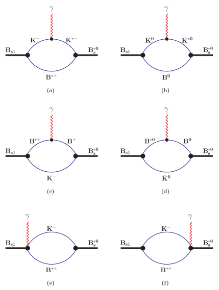
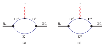
Figure 6: Diagrams contributing to the radiative transition $B_{s1}\to B_{s}^{\ast}+\gamma$.

Figure 7: Diagrams contributing to the radiative transition $B_{s1}\to B_{s0}^{\ast}+\gamma$.

References

- (1) J. L. Rosner, Phys. Rev. D 74, 076006 (2006) [arXiv:hep-ph/0608102].
- (2) T. Barnes, F. E. Close and H. J. Lipkin, Phys. Rev. D 68, 054006 (2003) [arXiv:hep-ph/0305025].
- (3) A. Faessler, T. Gutsche, V. E. Lyubovitskij and Y. L. Ma, Phys. Rev. D 76, 014005 (2007) [arXiv:0705.0254 [hep-ph]].
- (4) A. Faessler, T. Gutsche, S. Kovalenko and V. E. Lyubovitskij, Phys. Rev. D 76, 014003 (2007) [arXiv:0705.0892 [hep-ph]].
- (5) A. Faessler, T. Gutsche, V. E. Lyubovitskij and Y. L. Ma, Phys. Rev. D 76, 114008 (2007) [arXiv:0709.3946 [hep-ph]].
- (6) T. Branz, T. Gutsche and V. E. Lyubovitskij, arXiv:0712.0354 [hep-ph].
- (7) Y. B. Dong, A. Faessler, T. Gutsche and V. E. Lyubovitskij, in preparation.
- (8) S. Weinberg, Phys. Rev. 130, 776 (1963); A. Salam, Nuovo Cim. 25, 224 (1962); K. Hayashi, M. Hirayama, T. Muta, N. Seto and T. Shirafuji, Fortsch. Phys. 15, 625 (1967).
- (9) G. V. Efimov and M. A. Ivanov, The Quark Confinement Model of Hadrons, (IOP Publishing, Bristol Philadelphia, 1993).
- (10) I. V. Anikin, M. A. Ivanov, N. B. Kulimanova and V. E. Lyubovitskij, Z. Phys. C 65, 681 (1995); M. A. Ivanov, M. P. Locher and V. E. Lyubovitskij, Few Body Syst. 21, 131 (1996); M. A. Ivanov, V. E. Lyubovitskij, J. G. Körner and P. Kroll, Phys. Rev. D 56, 348 (1997) [arXiv:hep-ph/9612463]; M. A. Ivanov, J. G. Körner, V. E. Lyubovitskij and A. G. Rusetsky, Phys. Rev. D 60, 094002 (1999) [arXiv:hep-ph/9904421]; A. Faessler, T. Gutsche, M. A. Ivanov, V. E. Lyubovitskij and P. Wang, Phys. Rev. D 68, 014011 (2003) [arXiv:hep-ph/0304031]; A. Faessler, T. Gutsche, M. A. Ivanov, J. G. Korner, V. E. Lyubovitskij, D. Nicmorus and K. Pumsa-ard, Phys. Rev. D 73, 094013 (2006) [arXiv:hep-ph/0602193]; A. Faessler, T. Gutsche, B. R. Holstein, V. E. Lyubovitskij, D. Nicmorus and K. Pumsa-ard, Phys. Rev. D 74, 074010 (2006) [arXiv:hep-ph/0608015].
- (11) V. Baru, J. Haidenbauer, C. Hanhart, Yu. Kalashnikova and A. E. Kudryavtsev, Phys. Lett. B 586 (2004) 53 [arXiv:hep-ph/0308129]; C. Hanhart, Yu. S. Kalashnikova, A. E. Kudryavtsev and A. V. Nefediev, Phys. Rev. D 75, 074015 (2007) [arXiv:hep-ph/0701214].
- (12) S. Godfrey and R. Kokoski, Phys. Rev. D 43, 1679 (1991).
- (13) E. J. Eichten, C. T. Hill and C. Quigg, Phys. Rev. Lett. 71, 4116 (1993) [arXiv:hep-ph/9308337].
- (14) A. F. Falk and T. Mehen, Phys. Rev. D 53, 231 (1996) [arXiv:hep-ph/9507311].
- (15) D. Ebert, V. O. Galkin and R. N. Faustov, Phys. Rev. D 57, 5663 (1998) [Erratum-ibid. D 59, 019902 (1998)] [arXiv:hep-ph/9712318].
- (16) W. A. Bardeen, E. J. Eichten and C. T. Hill, Phys. Rev. D 68 (2003) 054024 [arXiv:hep-ph/0305049].
- (17) T. Matsuki, K. Mawatari, T. Morii and K. Sudoh, Phys. Lett. B 606 (2005) 329 [arXiv:hep-ph/0411034]; T. Matsuki and T. Morii, Phys. Rev. D 56, 5646 (1997) [Austral. J. Phys. 50, 163 (1997)] [arXiv:hep-ph/9702366].
- (18) E. E. Kolomeitsev and M. F. M. Lutz, Phys. Lett. B 582, 39 (2004) [arXiv:hep-ph/0307133].
- (19) T. Matsuki, T. Morii and K. Sudoh, AIP Conf. Proc. 814, 533 (2006) [arXiv:hep-ph/0510269].
- (20) F. K. Guo, P. N. Shen, H. C. Chiang and R. G. Ping, Phys. Lett. B 641 (2006) 278 [arXiv:hep-ph/0603072].
- (21) F. K. Guo, P. N. Shen and H. C. Chiang, Phys. Lett. B 647 (2007) 133 [arXiv:hep-ph/0610008].
- (22) P. Colangelo, F. De Fazio and R. Ferrandes, Nucl. Phys. Proc. Suppl. 163, 177 (2007) [arXiv:hep-ph/0609072].
- (23) J. Vijande, A. Valcarce and F. Fernandez, arXiv:0711.2359 [hep-ph].
- (24) Z. G. Wang, arXiv:0712.0118 [hep-ph].
- (25) F. K. Guo, S. Krewald and U. G. Meissner, arXiv:0712.2953 [hep-ph].
- (26) Z. G. Wang, arXiv:0801.0267 [hep-ph].
- (27) Z. G. Wang, arXiv:0801.1932 [hep-ph].
- (28) Z. G. Wang, arXiv:0803.1223 [hep-ph].
- (29) J. Gasser and H. Leutwyler, Nucl. Phys. B 250, 465 (1985).
- (30) P. L. Cho and M. B. Wise, Phys. Rev. D 49, 6228 (1994) [arXiv:hep-ph/9401301].
- (31) P. Colangelo and F. De Fazio, Phys. Lett. B 570, 180 (2003) [arXiv:hep-ph/0305140].
- (32) T. Mehen and R. P. Springer, Phys. Rev. D 70, 074014 (2004) [arXiv:hep-ph/0407181].
- (33) W. M. Yao et al. [Particle Data Group], J. Phys. G 33 (2006) 1.
- (34) S. Mandelstam, Annals Phys. 19, 1 (1962); J. Terning, Phys. Rev. D 44, 887 (1991).
- (35) Y. Dong, A. Faessler, T. Gutsche and V. E. Lyubovitskij, Phys. Rev. D 77, 094013 (2008) [arXiv:0802.3610 [hep-ph]].
- (36) A. Anastassov et al. [CLEO Collaboration], Phys. Rev. D 65, 032003 (2002) [arXiv:hep-ex/0108043].
- (37) Z. G. Wang and S. L. Wan, Phys. Rev. D 74, 014017 (2006) [arXiv:hep-ph/0606002].
- (38) M. E. Bracco, A. J. Cerqueira, M. Chiapparini, A. Lozea and M. Nielsen, Phys. Lett. B 641, 286 (2006) [arXiv:hep-ph/0604167].
- (39) F. S. Navarra, M. Nielsen and M. E. Bracco, Phys. Rev. D 65, 037502 (2002) [arXiv:hep-ph/0109188].
- (40) Z. W. Lin and C. M. Ko, Phys. Rev. C 62, 034903 (2000) [arXiv:nucl-th/9912046].
- (41) M. B. Wise, Phys. Rev. D 45, R2188 (1992).
- (42) R. Casalbuoni, A. Deandrea, N. Di Bartolomeo, R. Gatto, F. Feruglio and G. Nardulli, Phys. Rept. 281, 145 (1997) [arXiv:hep-ph/9605342].
- (43) J. A. M. Vermaseren, arXiv:math-ph/0010025.