Independent Emission and Absorption Abundances for Planetary Nebulae

Abstract

Emission-line abundances have been uncertain for more than a decade due to unexplained discrepancies in the relative intensities of the forbidden lines and weak permitted recombination lines in planetary nebulae (PNe) and H II regions. The observed intensities of forbidden and recombination lines originating from the same parent ion differ from their theoretical values by factors of more than an order of magnitude in some of these nebulae. In this study we observe UV resonance line absorption in the central stars of PNe produced by the nebular gas, and from the same ions that emit optical forbidden lines. We then compare the derived absorption column densities with the emission measures determined from ground-based observations of the nebular forbidden lines. We find for our sample of PNe that the collisionally excited forbidden lines yield column densities that are in basic agreement with the column densities derived for the same ions from the UV absorption lines. A similar comparison involving recombination line column densities produces poorer agreement, although near the limits of the formal uncertainties of the analyses. An additional sample of objects with larger abundance discrepancy factors will need to be studied before a stronger statement can be made that recombination line abundances are not correct.

1. Introduction

The analysis of emission line intensities has been used to determine nebular abundances for a wide range of objects. Standard procedures have been developed in which the collisionally excited forbidden lines and high-level permitted recombination lines of ions are used to determine abundances (Dopita & Sutherland, 2003; Osterbrock & Ferland, 2006). For most objects heavy element abundances are derived from the forbidden lines because of their greater strengths compared to the fainter recombination lines, which are frequently only marginally stronger than the continuum intensity. For some of the higher surface brightness gaseous nebulae both types of lines have been used to determine the heavy element CNO abundances, and they have produced discrepant results of more than an order of magnitude in some objects.

Each of the two types of lines have certain advantages for abundance determinations. The forbidden lines are strong, so they are detected from many more ions than the recombination lines. The collisional excitation of low-lying levels dominates other competing population processes such as fluorescence excitation, charge exchange, and dielectronic recombination. Furthermore, collision strengths coupling most of the lower bound levels of ions are known to better than 30% accuracy. The largest uncertainty in using forbidden line intensities for abundances is their sensitivity to kinetic temperature that results from excitation by electron impact.

Table 1Ions with UV Resonance and Optical Forbidden Lines

Ion	UV Resonance Transition $\lambda$(Å)	Optical Forbidden Line $\lambda$(Å)
C I	1277.5*, 1329.6*, 1561.4*, 1657.0*	4622, 8727, 9850
P II	1152.8, 1154.0*, 1301.9, 1310.7*, 1542.3*, 1532.5	4669, 7876
S I	1270.8, 1277.2, 1295.7, 1316.5, 1425.0, 1433.3*, 1474.0, 1483.0*, 1807.3, 1820.3*	4589, 7725
Fe II	1260.5, 1608.5, 1621.7*	4244, 4359, 5159, 8617
Ni II	1317.2, 1370.1, 1454.8, 1709.6, 1741.5	6667, 7378
N I	1199.5, 1200.2, 1200.7	3467, 5198, 5200, 10398
O I	1302.2, 1304.9*, 1306.0**	5577, 6300, 6364
S II	1250.6, 1253.8, 1259.5	4069, 4076, 6716, 6731, 10320
S III	1190.2, 1194.1*, 1201.7*	3722, 6312, 9069, 9531

Direct electron recapture populates the higher levels of ions and this process has relatively small cross sections. Thus, recombination lines tend not to be strong except for H and He by virtue of their dominant abundances, but they are observable in nebulae from ions of CNO and Ne. They have the advantage that recombination line intensity ratios are insensitive to temperature and density, and the relevant cross sections are believed to be known reasonably well. Because recombination cross sections are small, however, other excitation processes compete with electron recapture in populating the higher levels from which these lines are observed. Thus, there can be greater uncertainty in the excitation processes that are responsible for specific high level permitted lines.

Table 2Journal of Observations for HST UV Spectroscopy

Object	He2-138	NGC 246	NGC 6543	Tc 1
Central star (V)	10.9	11.9	11.1	11.4
Shell surface brightness, S(H$\beta$)
(erg cm-2 s-1 arcsec2)	5.1$\times 10^{-13}$	6.2$\times 10^{-16}$	8.2$\times 10^{-13}$	3.0$\times 10^{-13}$
Diameter of Central Nebular
Emission (arcsec)	7	245	20	10
Radial velocity, heliocentric (km s-1)	-47	-46	-66	-83
Exposure times (sec):
1150–1330Å	7$\times$2114	1967	2$\times$2150	2$\times$2072
				8$\times$1365
1316–1518Å	$\cdots$	2$\times$1368	2440	$\cdots$
1495–1688Å	7$\times$2116	$\cdots$	3$\times$2460	2077
				4$\times$1367

Electron temperatures and densities are determined directly from the relative intensities of forbidden lines originating on different levels of the same ion with the result that emission spectra have been a major source of our knowledge of element abundances of every type of emission-line object. The relatively high surface brightnesses of planetary nebulae and a few of the brighter H II regions enable the recombination lines of CNO to be observed, and in the past decade ion abundances have been determined for a number of PNe using both the forbidden lines (FL) and the recombination lines (RL) from the same ions. Surprisingly, the two types of lines have not yielded the same abundances. The differences between the RL and FL abundances vary from object to object and span the range from 15 percent, i.e., relatively good agreement, to factors of 50 and more (Tsamis et al., 2004; Robertson-Tessi & Garnett, 2005; Liu et al., 2006; Garcia-Rojas & Esteban, 2007), with the recombination line intensities always being stronger than predicted relative to the forbidden lines and therefore indicative of higher abundances. These discrepancies have been the subject of many studies which have given rise to a large literature on the subject, but they are still not understood. Until they are resolved some doubt is cast upon the normal methods by which collisionally excited forbidden lines are used to derive element abundances. The differences cannot be due to incorrect atomic data since this would cause the magnitude of the discrepancies to be roughly the same for all objects. Current resolutions to the discrepancies problem have focused on temperature fluctuations in the nebulae (Peimbert, 1967; Peimbert et al., 2004) and dense inclusions that are hydrogen deficient (Liu et al., 2000).

A completely independent, alternative method of obtaining abundances for nebular gas does exist and can be used as an independent check of emission-line abundances. It involves observing the absorption lines produced by the foreground nebular gas in the spectrum of an embedded or background star to determine column densities. Most of the absorption lines occur in the ultraviolet because low density gas occupies the ground state and the resonance lines of the most cosmically abundant ions fall in the UV. Thus, a space telescope with a high resolution spectrograph is required to study these absorption lines with sufficient resolution to yield reliable column densities.

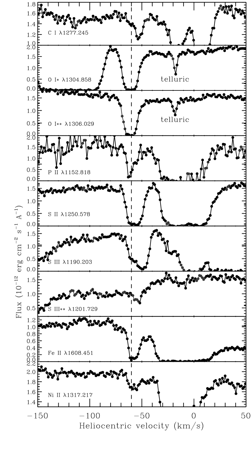
Figure 1.— A montage of UV absorption line profiles from HST/STIS spectra of the central star of He2-138. The foreground ISM absorption is centered around velocity = -10 km s^-1, and the PN shell absorption is centered around velocity = -60 km s^-1, as indicated by the vertical dashed line.

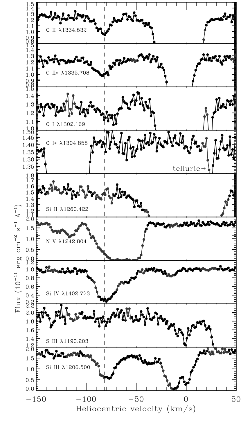
Figure 2.— A montage of UV absorption line profiles from the star of NGC 246 from the HST/STIS data. The ISM absorption is centered near velocity = 0, and the PN shell absorption is centered around velocity = -80 km s^-1, as indicated by the vertical dashed line. The broad N V absorption trough is indicative of an outflowing wind from the central star, which has a heliocentric velocity of v* = -46 km s^-1.

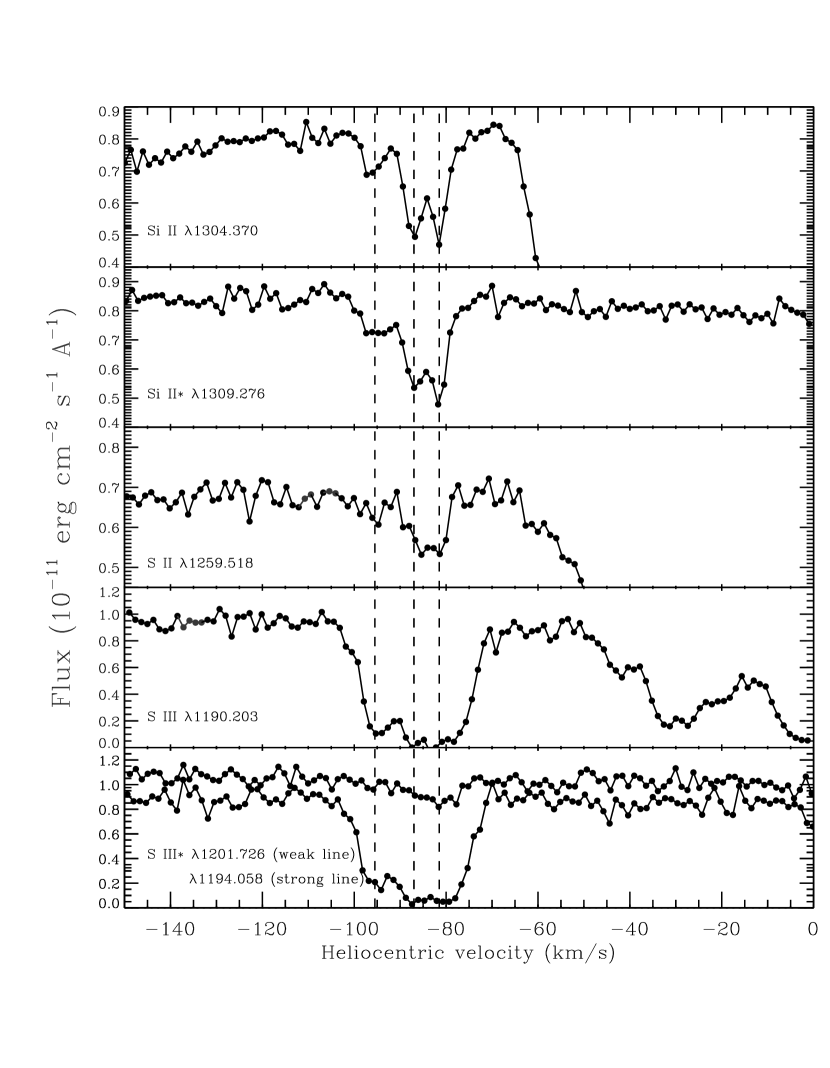
Figure 3.— Same as Figure 1 except for the central star NGC 6543. The three vertical dashed lines represent distinct absorption components from the nebular shell.

Pwa, Mo, & Pottasch (1984) and Pwa, Pottasch, Mo (1986) made the first attempts to obtain ion abundances in planetary nebulae by this method, using the IUE high resolution spectrograph (R=15,000) to measure absorption line equivalent widths from which column densities were determined. For the two PNe whose central stars were bright enough to be studied with IUE, the relatively few unsaturated lines for which they were able to obtain column densities belonged to ions that do not have detectable emission lines in the optical. Hence, although they did determine relative abundances from absorption line data, they were unable to make a direct comparison between independently derived absorption and emission line abundances for the same ions.

The high resolution spectrographs of HST increase the number of nebulae for which reliable column densities can be obtained, and offer the possibility of resolving the question of the abundance discrepancies. The more abundant heavy element ions having resonance lines in the UV between $\lambda\lambda$1150-1800Å accessible with the STIS spectrograph and also having detectable forbidden lines at optical wavelengths are listed in Table 1. The abundances of these ions can be determined independently from ground and space telescopes by completely different methods and then compared, albeit having separate sight lines and path lengths, e.g., the line of sight to the star does not probe the rear part of the nebula.

Specifically, the column densities of individual ions can be found from the UV absorption spectra, while emission measures are derived from the forbidden and permitted nebular emission lines. For each ion the column density and emission measure differ only by the multiplicative factor of the electron density in the emission measure. Since standard nebular diagnostics provide a direct determination of the density appropriate for each ion depending upon its ionization level, a direct comparison can be made between the absorption column density of the ion and its emission measure as derived from the different emission lines. This procedure should demonstrate which emission lines, forbidden or permitted, yield abundances most consistent with those from the UV absorption lines.

An initial study of abundances determined from UV absorption lines in the central star vs. those found from nebular emission line intensities for the PN IC 418 was attempted by Williams et al. (2003). For the four ions S⁺², S⁺, Ni⁺, and Fe⁺, and netural oxygen O^o, for which relative abundances could be determined independently from both methods, rough agreement was found. However, the uncertainties were too large for meaningful conclusions to be drawn.

We report here on an observing program which attempts to resolve the discrepancies between the forbidden and permitted emission line intensities by making a UV absorption line analysis that independently serves to validate emission line results. We have obtained high resolution UV spectra of four PNe central stars with HST/STIS, and visible spectra of three of the associated nebular shells from Las Campanas and KPNO. The UV observations and absorption analysis are described in §3, and the optical emission spectra and analysis are presented in §4. The relative column densities from the two methods are compared and interpreted in §5.

2. Object Sample and Observing Program

Column densities determined from absorption lines are most reliable when the lines are well-resolved and have ample signal-to-noise to define the continuum, thus brighter central stars are advantageous. Absorption lines originating in nebular gas are frequently seriously blended with and obliterated by stronger absorption from the same transitions caused by intervening ISM gas along the same line of sight. Unambiguous measurement of absorption from the nebular gas therefore requires a nebular radial velocity differing by at least 50 km s^-1 from that of the Local Standard of Rest to shift the nebular absorption out of the corresponding stronger ISM component. Optimal candidates for emission study are preferentially high surface brightness objects, thus favoring PNe over the lower surface brightness H II regions. It would be advantageous to include in our sample some PNe for which the largest FL and RL abundance discrepancies have been determined, however the few PNe that have been established to have differences of more than a factor of ten either have (a) central stars that are too faint in the UV, (b) very low surface brightnesses, or (c) radial velocities that are not sufficiently different from the LSR to avoid confusion between the nebular shell and ISM absorption lines.

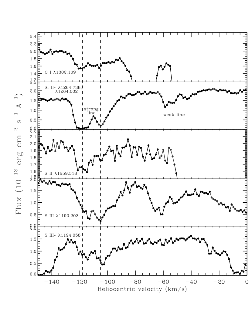
Figure 4.— Same as Figure 1, except for the central star of Tc 1.

The sample of known PNe satisfying the optimal criteria for study is given in Williams et al. (2003), and is not large. We identified four PNe that satisfy these criteria and which seem well suited for a combined UV-visible study, viz., He2-138, NGC 246, NGC 6543, & Tc 1, whose central stars are sufficiently bright that UV observations with HST at high spectral resolution would produce acceptable spectra in reasonable exposure times. We acquired spectra of the central stars of these PNe in the UV with HST/STIS and then subsequently observed the nebular shells along adjacent sight lines in the visible with ground-based telescopes to obtain line intensities for the emission-line analysis.

3. Absorption-Line Analysis

3.1. STIS Observations

HST/STIS was used to obtain spectra of the central stars of He2-138, NGC 246, NGC 6543, and Tc 1 in the high resolution mode, i.e., grating E140H with a resolution of 3 km s^-1, in three separate settings that covered the wavelength region 1150–1690 Å. Exposure times that produced a continuum signal-to-noise level of S/N$\approx$15 over the entire wavelength regime for each grating setting were adopted. The observations were made in 2005 (Cycle 12), and the relevant properties of our targets and the journal of the STIS observations is given in Table 2. Regrettably, STIS failed and became inoperative before our observing program could be completed, thus we did not succeed in executing all of our planned observations. Only partial data exist for each of the central stars. The spectra were reduced using the most recent version of CALSTIS procedures and algorithms (Lindler, 1998), and a montage of resonance line profiles from the final reduced spectra that include ions for which we also subsequently observed nebular forbidden emission lines is shown in Figures 1-4 for the four PNe.

3.2. UV Line Measurements

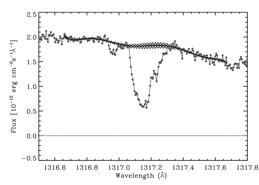
Figure 5.— A segment of the STIS spectrum that covers the Ni II line at 1317.217 Å for the central star in He2-138. The large feature centered at 1317.15 Å arises from foreground interstellar material. The small feature centered 1316.96 Å is the one that is relevant to our study, since it arises from the nebula. The adopted continuum level is shown by a curved line with a cross-hatched overlay that shows the 1$\sigma$ uncertainty in its placement.

Table 3 lists the absorption lines that we measured in the central star spectra of the four planetary nebulae. Following the name of each target in the subheaders of the table, we list the radial velocity of the central star $v_{*}$ and the velocity interval that covers the strongest absorption features that we identify as arising from the planetary nebula shell. Weaker features often spanned smaller velocity intervals and the measurements of these lines, along with those undetected, were taken over the more restricted ranges.

We defined the continuum levels by fitting Legendre polynomials to the fluxes on either side of each line, using the methods refined by Sembach & Savage (1992). In Figure 5 we present a portion of the UV spectrum of the He2-138 central star which shows the final continuum fit, together with the envelope defined by 1$\sigma$ excursions from the fit, used in the determination of the absorption intensities in the apparent optical depth analysis of the Ni II $\lambda$1317.217 line.

For each absorption feature, within the errors of the continuum fitting there is an acceptable range for the reconstructed intensity levels, and limits for this range defined the errors in the line measurements attributable to continuum uncertainties. For both the equivalent width measurements and the evaluations of column densities using the apparent optical depth (AOD) method (§3.3), we combined these continuum uncertainties in quadrature with the uncertainties due to photon-counting noise to arrive at a net error of the quantity being measured. In some instances, lines could be measured twice because they appeared in two adjacent echelle orders.

While our principal objective was to obtain column densities for ions in the nebular shells for comparison with emission line strengths from the same ions, we nevertheless have included in Table 3 measurements for absorption lines from ions for which there were no emission lines detected in our ground-based spectra (§4.2). We feel that it is prudent to include these lines for the benefit of future more general studies of the relative abundances of atoms and ions in the planetary nebulae shells.

Uncertain column densities result from either very weak lines that are marginally detected or strongly saturated lines. A few of the ions have multiple lines with a range of f-values that provide for reliable column densities. We avoided lines that were so badly saturated that their resulting lower limits for the column densities would be so much lower than the actual values that they would have no real value for any study. For some species, e.g., Mg II, only the strongest line appeared above the noise; for such cases we could not measure the weaker line. Using the same methods as for lines that were visible in our spectra, we evaluated intensity upper limits within the wavelength intervals where certain lines of interest might be expected, but which were either marginally detectable or not visible at all. Sometimes these measurements yielded negative equivalent widths, although with magnitudes comparable to or much less than the errors, and these determinations are ultimately useful in providing upper limits for the column densities (see footnote b to Table 3).

3.3. Absorption Column Densities

Column densities $N$ were derived by integrating over velocity the apparent optical depths $\tau_{a}(v)=\ln[I_{cont}(v)/I(v)]$ and evaluating the quantity

$$N\equiv\int n_{1}d\ell=m_{e}c/(\pi e^{2}f\lambda)\int\tau_{a}(v)dv\,,$$ (1)

where $n_{1}$ is the density of the ion in the lower level, and the numerical value for the expression in front of the integral is $3.77\times 10^{14}$ cm^-2 (km s^-1)^-1 (Savage & Sembach, 1991; Jenkins, 1996). The results for all of the ions with reliable determinations are given in Table 3, and it should be emphasized that the column densities refer only to those ions that occupy the lower level of the transition. Errors in the column densities may arise from three different sources: (a) photon-counting noise, (b) errors in the definition of the continuum level, and (c) errors in the adopted zero intensity level. If the random deviations of intensity arising from statistical fluctuations in photon counts are expressed as $\sigma_{I(v)}$, an approximation for the error in $\tau_{a}(v)$ is simply

$$\sigma_{\tau_{a}(v)}=\sigma_{I(v)}I_{cont}(v)/I(v)\,,$$ (2)

which is reasonably accurate as long as the quantity is much less than unity. Jenkins & Tripp (2001) found that for a signal-to-noise ratio of about 20 at the continuum (which applies to nearly all of our spectral lines) and a Gaussian error distribution, the approximation expressed in equation 2 is good as long as $I(v)/I_{cont}(v)\geq 0.15$. We have indicated which lines appearing in Table 3 violate this condition at the maximum level of absorption. For these cases, the upper error bounds may need to be increased to somewhat larger values than those listed.

The errors in optical depth $\sigma_{\tau_{a}(v)}$ that arise from photon counting are uncorrelated from one spectral element to the next, while the systematic error arising from a misplacement of the continuum is an effect that is usually coherent over the extent of an absorption feature. For this reason, the noise errors for successive spectral elements were added together in quadrature before they were combined as a group with the global uncertainty in line strength caused by inaccuracies in the definition of the continuum level. Since the errors arising from photon counting and continuum misplacement are uncorrelated, it is appropriate to add them together in quadrature. At the bottoms of severely saturated lines, we found that the intensities deviate from zero by less than 1% of the continuum intensity. Thus, anomalies arising from errors in zero corrections are insignificant compared to shortcomings of the approximation in equation 2.

Except for some strong lines of Si II and Si II* in the spectrum of NGC 6543, the values of $N$ obtained for lines of different strength generally agreed with each other. In this exception, the fact that the stronger lines yielded lower column densities than the weaker ones for these two ground state levels indicates that there are some unresolved saturated absorptions that make all of the evaluations of $N$ using equation 1 underestimate slightly the true value of $N$ for Si II (Jenkins, 1996).

4. Emission-Line Analysis

4.1. Optical Spectroscopy

Table 3Equivalent Widths and Column Densities

$\lambda$	$\log f\lambda$	Species	$W_{\lambda}$	$\log N$
(Å)			(mÅ)	$({\rm cm}^{-2}$)
He2-138  ($v_{*}=-47\,{\rm km~{}s}^{-1};~{}-73<v_{\rm PN}<-40\,{\rm km~{}s}^{-1}$)
1656.928	2.392	C I	$28.6\pm 4.4$	12.97 ($+0.07,-0.08$)
1560.309	2.082	C I	$2.6\pm 1.8$	12.25 ($+0.22,-0.47$)
1277.245	2.037	C I	$11.2\pm 1.8$	13.00 ($+0.07,-0.08$)
1548.204	2.468	C IV	$32.5\pm 4.2$	12.99 ($+0.06,-0.07$)
1550.781	2.167	C IV	$15.7\pm 4.0$	12.93 ($+0.10,-0.13$)
1550.781	2.167	C IV	$11.8\pm 2.6$	12.79 ($+0.09,-0.11$)
1304.858	1.795	O I*	$75.1\pm 1.2$	14.49 ($+0.05,-0.05$)
1306.029	1.795	O I**	$64.9\pm 1.4$	14.38 ($+0.04,-0.04$)
1306.029	1.795	O I**	$67.7\pm 2.2$	14.20 ($+0.08,-0.10$)
1239.925	-0.106	Mg II	$5.0\pm 1.3$	14.79 ($+0.10,-0.14$)
1239.925	-0.106	Mg II	$4.2\pm 1.1$	14.72 ($+0.10,-0.14$)
1670.789	3.463	Al II	$91.4\pm 20.5$	12.69 ($+0.12,-0.17$)
1304.370	2.052	Si II	$88.9\pm 1.0$	14.57 ($+0.04,-0.05$)
1309.276	2.052	Si II*	$69.6\pm 2.3$	13.98 ($+0.02,-0.02$)
1309.276	2.052	Si II*	$71.5\pm 2.4$	13.98 ($+0.02,-0.02$)
1152.818	2.451	P II	$31.2\pm 3.8$	13.28 ($+0.09,-0.11$)
1301.874	1.219	P II	$4.1\pm 1.1$	13.36 ($+0.11,-0.14$)
1153.995	2.331	P II**	$11.2\pm 4.5$	12.83 ($+0.14,-0.22$)
1295.653	2.052	S I	$1.6\pm 1.6$	$<12.58$
1250.578	0.832	S II	$74.9\pm 2.0$	15.49 ($+0.08,-0.09$)
1250.578	0.832	S II	$71.7\pm 1.2$	15.42 ($+0.10,-0.14$)
1190.203	1.449	S III	$73.6\pm 2.3$	14.76 ($+0.12,-0.16$)
1190.203	1.449	S III	$70.0\pm 1.6$	14.70 ($+0.02,-0.02$)
1201.729	0.626	S III**	$16.3\pm 3.2$	14.63 ($+0.08,-0.10$)
1197.184	2.414	Mn II	$9.4\pm 2.5$	12.66 ($+0.11,-0.15$)
1197.184	2.414	Mn II	$10.8\pm 2.2$	12.68 ($+0.08,-0.10$)
1199.391	2.308	Mn II	$6.2\pm 2.5$	12.53 ($+0.14,-0.22$)
1608.451	1.968	Fe II	$55.0\pm 2.3$	13.95 ($+0.03,-0.04$)
1317.217	1.876	Ni II	$4.1\pm 1.3$	12.70 ($+0.12,-0.16$)
1317.217	1.876	Ni II	$5.3\pm 1.1$	12.81 ($+0.09,-0.11$)
1237.059	3.183	Ge II	$9.7\pm 1.3$	11.86 ($+0.06,-0.06$)
1237.059	3.183	Ge II	$11.6\pm 1.2$	11.94 ($+0.05,-0.05$)
1235.838	2.402	Kr I	$3.4\pm 1.9$	12.14 ($+0.18,-0.33$)
1235.838	2.402	Kr I	$4.6\pm 1.2$	12.25 ($+0.10,-0.14$)
NGC 246  ($v_{*}=-46\,{\rm km~{}s}^{-1};~{}-95<v_{\rm PN}<-60\,{\rm km~{}s}^{-1}$)
1277.245	2.037	C I	$0.2\pm 1.0$	$<12.29$
1334.532	2.234	C II	$12.9\pm 1.1$	12.84 ($+0.04,-0.04$)
1334.532	2.234	C II	$14.3\pm 1.0$	12.89 ($+0.03,-0.03$)
1335.708	2.234	C II*	$15.8\pm 1.0$	12.93 ($+0.03,-0.03$)
1199.550	2.199	N I	$-0.7\pm 1.0$	$<12.04$
1302.169	1.796	O I	$4.3\pm 2.1$	12.80 ($+0.17,-0.28$)
1302.169	1.796	O I	$0.6\pm 1.7$	$<12.78$
1304.858	1.795	O I*	$-1.7\pm 1.3$	$<12.44$
1260.422	3.171	Si II	$6.5\pm 2.6$	11.61 ($+0.14,-0.22$)
1264.738	3.125	SiII*	$-0.3\pm 1.0$	$<11.14$
1206.500	3.293	Si III	$49.7\pm 3.5$	12.52 ($+0.03,-0.03$)
1393.760	2.854	Si IV	$145.1\pm 2.3$	13.50 ($+0.01,-0.01$)
1402.773	2.552	Si IV	$97.6\pm 1.3$	13.51 ($+0.01,-0.01$)
1259.518	1.320	S II	$3.5\pm 2.2$	13.19 ($+0.20,-0.40$)
1190.203	1.449	S III	$3.4\pm 1.3$	13.08 ($+0.14,-0.21$)
1194.058	1.325	S III*	$-1.7\pm 2.5$	$<13.32$
1317.217	1.876	Ni II	$2.1\pm 1.8$	12.40 ($+0.26,-0.71$)
1370.132	1.906	Ni II	$-0.6\pm 1.9$	$<12.61$
NGC 6543  ($v_{*}=-66\,{\rm km~{}s}^{-1};~{}-103<v_{\rm PN}<-74\,{\rm km~{}s}^{-1}$)
1277.245	2.037	C I	$1.1\pm 1.4$	$<12.52$
1200.223	2.018	N I	$2.0\pm 1.7$	12.29 ($+0.25,-0.69$)
1304.858	1.795	O I*	$1.7\pm 1.3$	12.39 ($+0.25,-0.65$)
1306.029	1.795	O I**	$-0.3\pm 1.8$	$<12.73$
1306.029	1.795	O I**	$-1.4\pm 1.3$	$<12.47$
1670.789	3.463	Al II	$6.5\pm 4.5$	11.22 ($+0.22,-0.48$)
1260.422	3.171	Si II	$85.9\pm 1.6$	13.11 ($+0.02,-0.02$)
1526.707	2.307	Si II	$35.7\pm 2.0$	13.23 ($+0.03,-0.03$)
1304.370	2.052	Si II	$19.8\pm 1.4$	13.25 ($+0.03,-0.03$)
1264.738	3.125	Si II*	$88.8\pm 0.9$	13.17 ($+0.02,-0.02$)

Table 3(continued)

$\lambda$	$\log f\lambda$	Species	$W_{\lambda}$	$\log N$
(Å)			(mÅ)	$({\rm cm}^{-2}$)
NGC 6543  ($v_{*}=-66\,{\rm km~{}s}^{-1};~{}-103<v_{\rm PN}<-74\,{\rm km~{}s}^{-1}$)
1533.432	2.307	Si II*	$43.5\pm 2.9$	13.33 ($+0.03,-0.03$)
1265.002	2.171	Si II*	$33.2\pm 1.5$	13.39 ($+0.02,-0.02$)
1309.276	2.052	Si II*	$22.6\pm 1.0$	13.31 ($+0.02,-0.02$)
1152.818	2.451	P II	$5.8\pm 6.2$	$<12.81$
1259.518	1.320	S II	$9.6\pm 2.4$	13.65 ($+0.10,-0.12$)
1253.805	1.136	S II	$6.3\pm 1.3$	13.64 ($+0.08,-0.10$)
1190.203	1.449	S III	$93.2\pm 1.4$	14.92 ($+0.29,-1.33$)
1194.058	1.325	S III*	$87.2\pm 1.7$	14.96 ($+0.02,-0.03$)
1194.058	1.325	S III*	$86.5\pm 1.6$	14.95 ($+0.02,-0.02$)
1197.184	2.414	Mn II	$1.3\pm 2.1$	$<12.32$
1199.391	2.308	Mn II	$0.2\pm 2.2$	$<12.38$
1608.451	1.968	Fe II	$0.1\pm 4.0$	$<12.84$
1317.217	1.876	Ni II	$-0.7\pm 1.6$	$<12.56$
1370.132	1.906	Ni II	$-1.2\pm 2.2$	$<12.64$
Tc 1  ($v_{*}=-83\,{\rm km~{}s}^{-1};~{}-128<v_{\rm PN}<-86\,{\rm km~{}s}^{-1}$)
1560.309	2.082	C I	$-3.2\pm 4.1$	$<12.65$
1277.245	2.037	C I	$-1.9\pm 2.4$	$<12.54$
1199.550	2.199	N I	$-2.1\pm 3.1$	$<12.53$
1302.169	1.796	O I	$27.1\pm 2.4$	13.63 ($+0.04,-0.04$)
1306.029	1.795	O I**	$0.5\pm 2.0$	$<12.83$
1239.925	-0.106	Mg II	$0.2\pm 3.2$	$<14.94$
1239.925	-0.106	Mg II	$7.2\pm 3.8$	14.94 ($+0.18,-0.32$)
1670.787	3.463	Al II	$74.8\pm 22.9$	12.34 ($+0.12,-0.16$)
1260.422	3.171	Si II	$110.7\pm 2.1$	13.22 ($+0.02,-0.02$)
1193.290	2.842	Si II	$66.9\pm 3.7$	13.17 ($+0.03,-0.03$)
1190.416	2.541	Si II	$38.1\pm 4.4$	13.15 ($+0.05,-0.05$)
1304.370	2.052	Si II	$22.3\pm 1.2$	13.29 ($+0.02,-0.03$)
1264.738	3.125	Si II*	$99.8\pm 1.7$	13.18 ($+0.02,-0.02$)
1265.002	2.171	Si II*	$22.9\pm 2.4$	13.20 ($+0.04,-0.05$)
1309.276	2.052	Si II*	$22.8\pm 1.7$	13.29 ($+0.03,-0.03$)
1152.818	2.451	P II	$7.3\pm 6.9$	12.52 ($+0.25,-0.66$)
1259.518	1.320	S II	$10.3\pm 2.0$	13.67 ($+0.08,-0.09$)
1190.203	1.449	S III	$79.9\pm 2.6$	14.65 ($+0.02,-0.02$)
1194.058	1.325	S III*	$49.5\pm 5.6$	14.46 ($+0.05,-0.06$)
1194.058	1.325	S III*	$48.4\pm 6.2$	14.46 ($+0.06,-0.07$)
1197.184	2.414	Mn II	$25.8\pm 4.8$	13.06 ($+0.08,-0.09$)
1197.184	2.414	Mn II	$25.9\pm 2.9$	13.05 ($+0.05,-0.05$)
1608.451	1.968	Fe II	$-2.9\pm 8.5$	$<13.12$
1317.217	1.876	Ni II	$0.4\pm 1.4$	$<12.60$
1237.059	3.183	Ge II	$-5.3\pm 3.2$	$<11.43$
1237.059	3.183	Ge II	$-2.4\pm 3.8$	$<11.63$
1235.838	2.402	Kr I	$9.0\pm 2.6$	12.53 ($+0.11,-0.15$)

Table 3(continued)

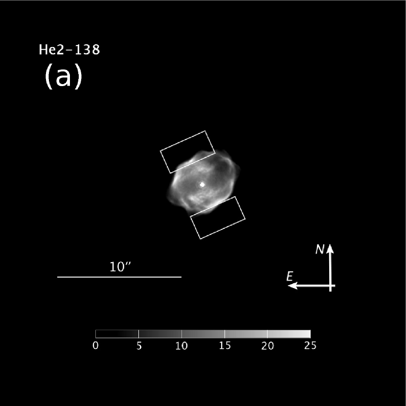
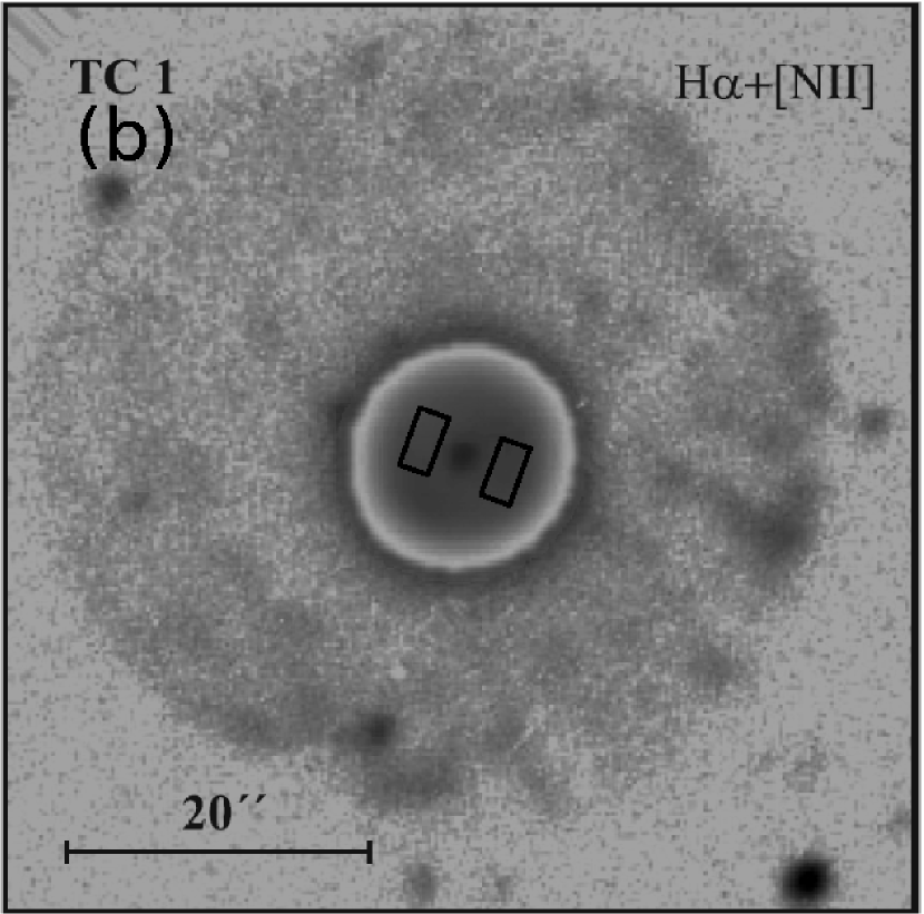
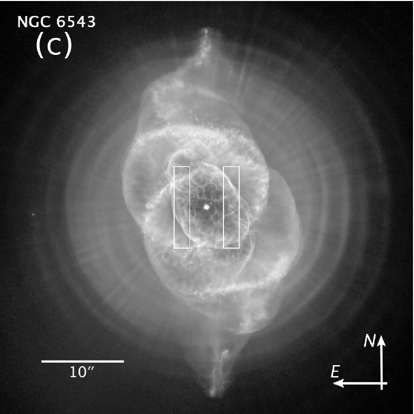
Figure 6.— Images of program PNe showing locations, orientations, and size of slits for (a) He2-138, (b) Tc1, and (c) NGC 6543. In all figures North is up and East is to left. Panels (a) and (c) are HST images. The shell emission sampled by our spectra would be represented by these images convolved with a 1–1.3 arcsec PSF.

The four PNe studied here were observed in the visible with ground-based telescopes to measure intensities of the nebular emission lines. The lower surface brightnesses of the nebular shells compared with the central stars dictated that the nebular spectra sight lines be positioned no closer than 2 arcsec from the central star in order to avoid unacceptable levels of contamination by scattered light from the brighter star. However, our goal was to estimate the intensity directly along the line of sight to the central star since this is the position of the gas that produces the absorption lines. Our approach was to take spectra in two positions symmetrically placed on either side of the central star and to then average together the two spectra after they had been flux calibrated. The flux average serves to compensate for surface brightness fluctuations, but does not represent the flux along the sight line to the central star if there is a radial gradient in surface brightness away from the central star due to the three-dimensional structure of the shell.

Initially, a reconnaissance was carried out in 2004 at low spectral resolution (300–500 km s^-1 FWHM) using the Gold Spectrograph on the 2.1m telescope at Kitt Peak National Observatory (KPNO) to observe NGC 246 and NGC 6543, and the Wide Field CCD (WFCCD) camera on the du Pont 2.5m telescope at Las Campanas Observatory (LCO) to observe He2-138, NGC 246, and Tc 1. We found that the emission lines in NGC 246 are much too faint for accurate spectrophotometric measurements of any of the weaker emission lines; only a few of the very strongest lines such as [O III] $\lambda$5007 were visible even in long exposures. This object was therefore removed from our program, but we provide the UV information from the central star spectrum in this paper because of its potential use for abundance studies. The visible spectra of the nebulae showed that line blending dictated the need for much higher resolution data to show many of the weaker emission lines of interest in the other three objects. This led us to obtain 15–20 km s^-1 FWHM resolution echelle spectra in 2005 with the echelle spectrographs on the 4m Mayall Telescope at KPNO and the 2.5m du Pont Telescope at LCO.

4.1.1 Observations at LCO

The LCO echelle spectrograph uses a prism as a cross disperser and covers the wavelength range $\lambda\lambda$3480–10,150Å in 64 orders, with increasingly large wavelength gaps between orders beyond $\lambda$8000Å. On each of the two nights 8, 9 June 2005 UT, we observed He2-138 and Tc 1 in two different slit positions symmetrically placed on either side of the central star, using a 2 arcsec wide $\times$ 4 arcsec long slit and offsetting at an angle so that the slit would include the brightest part of the nebulae. The slit orientations were at right angles to the directions of the offsets. The two slit positions for Tc 1 were 1.0 arcsec S, 2.7 arcsec W of the central star, and 1.0 arcsec N, 2.7 arcsec E. For He2-138, the two slit positions were 2.7 arcsec N, 1.25 arcsec E and 2.7 arcsec S, 1.25 arcsec W of the central star. The slit positions used for our observations are shown in Figure 6, overlayed on the best available images that we could find for these objects.

For Tc 1 the spectra were taken well inside the outer edge of the nebula. However, for the smaller He2-138 we were not able to simultaneously avoid the scattering effects of the central star and sample the shell well inside its outer edge, so the slit had to be placed near the outer edge of the nebula. Figure 6a shows a Hubble Telescope image of He2-138 with the spectrograph slit positions superposed. Atmospheric seeing resulted in shell emission filling the central portion of the slit. We detected flux along the central 3 arcsec of the slit, but variations in tracking and seeing caused the intensity to vary among the exposures. These variations make our determinations of the emission measure for this object considerably less certain than for the other two PNe. The spectral resolution was 15 km s^-1 FWHM over most of the range, but degraded to 20 km s^-1 at the extreme ends. We extracted spectra from each position, and after applying the proper flux calibration averaged the two extracted spectra together. We added together seven 1200 sec exposures at each slit position over two nights to measure the weak lines, and used pairs of 30 or 60 sec exposures at each position to measure the strong emission lines which would otherwise be saturated.

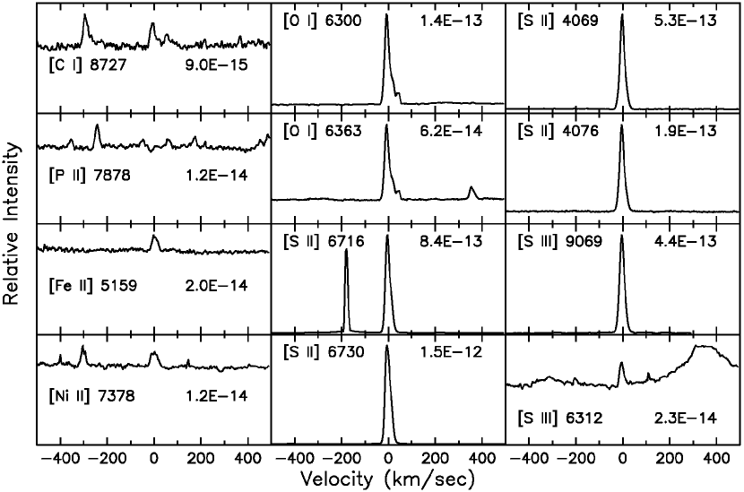
Figure 7.— Nebular emission line profiles from the LCO echelle spectrum of He2-138. The panels show the forbidden emission lines listed in Table 7 that were used to determine forbidden line abundances. The corresponding lines are shown at zero velocity in each panel. The linear vertical scale is F_λ in units of erg cm^-2 s^-1 Å^-1 with the bottom abscissa of each panel corresponding to zero flux and the top corresponding to the value of F_λ printed inside the panel.

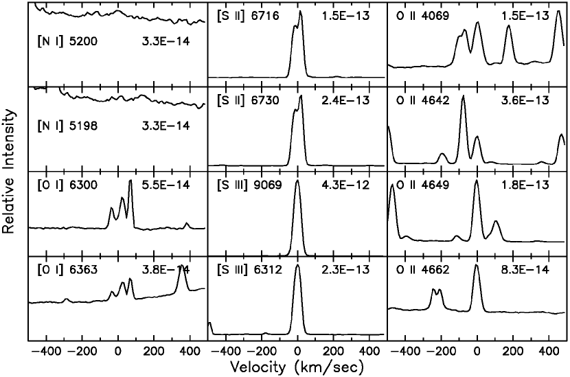
Figure 8.— Emission line profiles from the KPNO echelle spectrum of NGC 6543. The panels and scaling are as in Figure 7, except that the right-hand column shows four of the stronger O II recombination lines from Table 10. The stronger red [O I] emission components at +70 km s^-1 are atmospheric airglow lines.

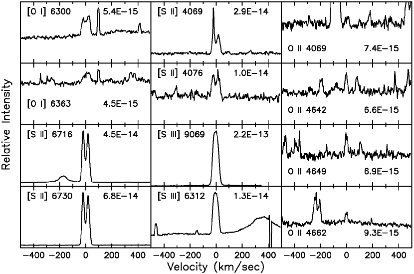
Figure 9.— Emission line profiles from the LCO echelle spectrum of Tc 1. The panels and scaling are as in Figure 7, with the narrow [O I] components at +100 km s^-1 again due to atmospheric [O I] emisison.

Only the second night was photometric so we used observations of the standard stars HR 4468, HR 4963 and HR 5501 (Hamuy et al., 1994) made through a 8$\times$8 arcsec slit on the second night to calibrate both nights. We applied this calibration in three steps. We first added together the raw counts from all of the different long exposures, which is the optimal weighting for detecting weak lines, and then flux calibrated that spectrum using a mean airmass. This gave a high signal-to-noise ratio spectrum that was affected by a wavelength-independent attenuation and by a slight error in the wavelength dependence of the extinction correction. The second step was to properly flux calibrate a single long exposure in each slit position on the photometric night using the correct airmass. Finally, we measured the fluxes of the same intermediate strength emission lines in both spectra, and used the flux ratios to correct the high S/N spectrum to match the flux scale of the single well-calibrated spectrum. This procedure provides the best calibration for our observing circumstances and results in absolute spectrophotometry accurate to better than 8 percent over the whole wavelength range.

4.1.2 Observations at KPNO

Table 4Optical Forbidden Emission Line Fluxes

		He2-138		NGC 6543		Tc 1
Species	$\lambda$(Å)	$F$	$F_{c}$	$F$	$F_{c}$	$F$	$F_{c}$
H I	4861	3.49(-12)	1.26(-11)	1.51(-11)	2.10(-11)	1.58(-12)	3.37(-12)
C I	4622	2.76(-16):	1.07(-15):	$\cdots$	$\cdots$	$\cdots$	$\cdots$
C I	8727	1.63(-15)	2.86(-15)	$\cdots$	$\cdots$	$<$1.97(-16)	$<$2.76(-16)
C I	9824	1.16(-15):	1.84(-15):	$\cdots$	$\cdots$	$\cdots$	$\cdots$
C I	9850	$\cdots$	$\cdots$	$\cdots$	$\cdots$	$<$9.74(-16)	$<$1.28(-15)
N I	5198	3.08(-14)	9.97(-14)	4.37(-15):	5.92(-15):	3.79(-16):	7.61(-16):
N I	5200	1.88(-14)	6.09(-14)	3.92(-15):	5.30(-15):	4.04(-16):	8.10(-16):
N II	5755	3.60(-14)	1.01(-13)	4.70(-14)	6.13(-14)	2.00(-14)	3.68(-14)
N II	6548	3.08(-12)	7.37(-12)	7.66(-13)	9.59(-13)	6.17(-13)	1.04(-12)
N II	6583	9.38(-12)	2.23(-11)	2.55(-12)	3.18(-12)	1.92(-12)	3.21(-12)
O I	5577	6.33(-16)	1.84(-15)	$\cdots$	$\cdots$	6.61(-17):	1.25(-16):
O I	6300	7.36(-14)	1.85(-13)	2.12(-14)	2.69(-14)	2.45(-15)	4.24(-15)
O I	6364	2.66(-14)	6.60(-14)	7.03(-15)	8.82(-15)	9.68(-16)	1.66(-15)
O II	3726	4.51(-13)	2.25(-12)	1.40(-12)	2.12(-12)	1.68(-12)	4.36(-12)
O II	3729	2.00(-13)	9.97(-13)	6.41(-13)	9.70(-13)	1.11(-12)	2.90(-12)
O II	7320	5.02(-12)	1.06(-13)	1.74(-13)	2.10(-13)	1.21(-13)	1.89(-13)
O II	7330	4.74(-14)	9.97(-14)	1.79(-13)	2.17(-13)	1.02(-13)	1.59(-13)
O III	4363	$<$6.29(-16)	$<$2.64(-15)	3.73(-13)	5.40(-13)	7.97(-15)	1.87(-14)
O III	4959	5.72(-16)	1.99(-15)	4.15(-11)	5.73(-11)	6.72(-13)	1.41(-12)
O III	5007	2.72(-15)	9.34(-15)	1.24(-10)	1.71(-10)	2.00(-12)	4.17(-12)
P II	4669	$<$6.29(-16)	$<$2.40(-15)	$\cdots$	$\cdots$	$<$2.07(-16)	$<$4.58(-16)
P II	7876	1.20(-16)	2.34(-16)	$\cdots$	$\cdots$	$<$5.98(-17)	$<$8.88(-17)
S I	4589	$<$8.88(-16)	$<$3.48(-15)	$\cdots$	$\cdots$	$<$2.07(-16)	$<$4.66(-16)
S I	7725	$\cdots$	$\cdots$	$\cdots$	$\cdots$	$<$7.99(-17)	$<$1.20(-16)
S II	4069	1.23(-13)	5.64(-13)	6.84(-14)	1.01(-13)	8.36(-15)	2.06(-14)
S II	4076	4.47(-14)	2.04(-13)	1.24(-14)	1.83(-14)	2.40(-15)	5.91(-15)
S II	6716	4.69(-13)	1.09(-12)	1.38(-13)	1.71(-13)	4.50(-14)	7.43(-14)
S II	6731	9.77(-13)	2.26(-12)	2.54(-13)	3.15(-13)	7.15(-14)	1.18(-13)
S III	6312	2.24(-15)	5.60(-15)	1.71(-13)	2.17(-13)	9.22(-15)	1.59(-14)
S III	9069	3.44(-13)	5.85(-13)	4.91(-12)	5.63(-12)	3.19(-13)	4.38(-13)
Cl III	5518	4.57(-16)	1.35(-15)	6.54(-14)	8.65(-14)	5.06(-15)	9.62(-15)
Cl III	5538	7.90(-16)	2.32(-15)	9.27(-14)	1.22(-13)	5.39(-15)	1.02(-14)
Ar III	5192	$\cdots$	$\cdots$	1.05(-14)	1.42(-14)	5.29(-16)	1.06(-15)
Ar III	7136	2.78(-15)	6.02(-15)	3.56(-12)	4.35(-12)	1.53(-13)	2.42(-13)
Ar III	7751	3.75(-16)	7.34(-16)	8.30(-13)	9.89(-13)	3.85(-14)	5.78(-14)
Ar IV	4711	$\cdots$	$\cdots$	1.77(-13)	2.49(-13)	$\cdots$	$\cdots$
Ar IV	4740	$\cdots$	$\cdots$	2.08(-13)	2.92(-13)	$\cdots$	$\cdots$
Fe II	4244	$<$1.44(-15)	$<$6.28(-15)	1.10(-15):	1.61(-15):	$<$3.12(-16)	$<7$.47(-16)
Fe II	4359	3.56(-15)	1.50(-14):	1.39(-15):	2.01(-15):	$<$2.08(-16)	$<$4.87(-16)
Fe II	5159	1.58(-15)	5.17(-15):	$\cdots$	$\cdots$	$\cdots$	$\cdots$
Fe II	8617	2.75(-15)	4.91(-15):	$\cdots$	$\cdots$	$<$1.98(-16)	$<$2.78(-16)
Ni II	6667	1.49(-15):	3.48(-15):	4.69(-16):	5.83(-16):	2.29(-16):	3.80(-16):
Ni II	7376	1.71(-15):	3.58(-15):	$\cdots$	$\cdots$	$<$1.00(-16)	$<$1.55(-16)

The KPNO echelle spectra of NGC 6543 were taken over the three nights 18-20 June 2005 UT. We used the UV camera on the 4m Mayall Telescope Cassegrain echelle spectrograph with echelle grating 79-63 and cross disperser 226-1 with two different setups, each giving 20 km s^-1 resolution. The blue setup, used for the first two nights, covered the wavelength range $\lambda\lambda$3200–5300Å. It used the cross disperser in second order with a CuSO₄ order separating filter. We then switched to a red setup covering the range $\lambda\lambda$4750–9900Å in first order of the cross-disperser grating, using a GG495 order separating filter. For calibration we observed standard stars HR 4468, HR 4963, HR 5501 and HR 8634 from Hamuy et al. (1994), measured through a 6 arcsec wide slit. The nights with the blue setup were photometric, while there were some clouds present when we used the red setup. We used the measured strengths of emission lines in the overlapping sections of the red and blue spectra to scale the fluxes for the red spectra to match those of the blue spectrum.

As was done at LCO, spectra were taken in two positions symmetrically placed on either side of the central star. In this case the slit was 2 arcsec wide by 10 arcsec long and was centered 3 arcsec to the E and then 3 arcsec to the W of the central star with a slit position angle of 90^o, as shown in Figure 6. As with Tc 1 these slit positions are well inside the outer regions of the nebula. The combined exposure times at each slit position for each grating setting were of order 60 min. We flux calibrated the NGC 6543 spectra and then averaged together the two slit positions to get a final spectrum interpolated for the line of sight to the central star in the same way as was done with the LCO spectra. We determine the absolute spectrophotometry of our calibration to have an accuracy of better than 7 percent. In Figures 7-9 we show portions of the nebular spectra of the three PNe that were used in the analysis of the emission lines and which show both the strong diagnostic forbidden lines and the weaker recombination lines of O II.

4.2. Nebular Emission Line Intensities

The emission line fluxes have been measured from the final co-added and averaged spectra using the IRAF splot routine. The measurements were straightforward because few of the lines of interest showed evidence of significant blending. The resultant observed intensities for He2-138, NGC 6543, and Tc 1 are given in Table 4 for lines that can be used to obtain $T_{e}$, $n_{e}$, and extinction along the lines of sight. The observed intensities have been corrected for extinction by taking the flux ratios of multiple unblended Balmer and Paschen line pairs from the same upper levels and determining the logarithmic extinction at H$\beta$, c_Hβ, from the expression

$$c_{H\beta}=\left[X_{H\beta}/(X_{1}-X_{2})\right]\times\log_{10}\left(A_{1}F_{2}\lambda_{2}/A_{2}F_{1}\lambda_{1}\right)\,,$$ (3)

where $A_{1,2}$, $\lambda_{1,2}$, and $F_{1,2}$ are the spontaneous emission coefficients, wavelengths, and observed fluxes for a specific Balmer and Paschen line pair, and $X_{1,2,H\beta}$ are the galactic extinction law values fitted by Howarth (1983) at the wavelengths of the lines and H$\beta$ respectively (assuming $R=3.2$). Individual emission line fluxes were then corrected using the relation

$$F_{c}(\lambda)=10^{c_{H\beta}X(\lambda)/X_{H\beta}}F(\lambda)\,,$$ (4)

where $F_{c}$ is the corrected flux. Taking the average of values obtained from multiple line pairs for our lines of sight we derive values of c_Hβ = 0.56, 0.14, and 0.33 for He2-138, NGC 6543, and Tc 1. These values are in good agreement with those of Cahn, Kaler, & Stanghellini (1992), who obtained global values of 0.40, 0.12, and 0.28 for the three PNe. The extinction corrected fluxes, $F_{c}$, are listed in column 4 of Table 4, including the upper limits to fluxes of undetected lines, which have been taken to be the 3$\sigma$ rms flux of the noise of the neighboring continuum.

4.3. Plasma Diagnostics and Emission Measures

Table 5Atomic Data References

Species	Transition Probabilities	Collision Strengths
C I	Nussbaumer & Rusca (1979)	Pequignot & Aldrovandi (1976)
	Froese Fischer & Saha (1985)	Thomas & Nesbet (1975)
		Johnson, Burke, & Kingston (1987)
N I	Zeippen (1982)	Berrington & Burke (1981)
	Froese Fischer & Tachiev (2004)	Dopita, Mason, & Robb (1976)
N II	Nussbaumer & Rusca (1979)	Stafford et al. (1994)
	Wiese, Fuhr, & Deters (1996)	Saraph, Seaton, & Shemming (1969)
		Lennon & Burke (1994)
O I	Baluja & Zeippen (1988)	Berrington & Burke (1981)
	Mendoza (1983)	Berrington (1988)
		LeDourneuf & Nesbet (1976)
O II	Zeippen (1982)	Pradhan (1976)
	Wiese, Fuhr, & Deters (1996)	McLaughlin & Bell (1993)
O III	Nussbaumer & Storey (1981)	Aggarwal (1983)
	Wiese, Fuhr, & Deters (1996)	Aggarwal, Baluja, & Tully (1982)
		Baluja, Burke, & Kingston (1980)
		Baluja, Burke, & Kingston (1981)
		Lennon & Burke (1994)
P II	Kaufman & Sugar (1986)	Tayal (2004)
	Mendoza & Zeippen (1982b)	Kruger & Czyzak (1970)
S II	Mendoza & Zeippen (1982a)	Keenan et al. (1996)
	Keenan et al. (1993)	Mendoza (1982)
	Verner, Verner, & Ferland (1996)
S III	Mendoza & Zeippen (1982b)	Mendoza (1982)
	Heise, Smith, & Calamai (1995)
	LaJohn & Luke (1993)
Cl III	Mendoza & Zeippen (1982a)	Butler & Zeippen (1989)
Ar III	Mendoza & Zeippen (1983)	Johnson & Kingston (1990)
		Kruger & Czyzak (1970)
Ar IV	Mendoza & Zeippen (1982a)	Zeippen, Le Borlot, & Butler (1987)
	Kaufman & Sugar (1986)
Fe II	Nussbaumer & Storey (1988)	Zhang & Pradhan (1995)
(159 levels)	Garstang (1962)	Bautista & Pradhan (1996)
	Nahar (1995)	Bautista & Kallman (2001)
	Schnabel, Schultz-Johanning, & Kock (2004)
	Bautista & Kallman (2001)
Ni II	Nussbaumer & Storey (1982)	Bautista (2004)
(76 levels)	Kurucz (1992)

Table 6Electron Temperatures and Densities

Diagnostic	He2-138	NGC 6543	Tc 1
Density (cm-3)
[N I] $\lambda$5198/$\lambda$5200	7000${}^{+\infty}_{-6000}$	900${}^{+900}_{-500}$	400${}^{600}_{-300}$
[S II] $\lambda$6716/$\lambda$6731	15000	5000${}^{+17000}_{-3000}$	3000${}^{+3800}_{-1200}$
[O II] $\lambda$3726/$\lambda$3729	7500${}^{+9000}_{-3000}$	6000${}^{+2400}_{-1600}$	2000${}^{+800}_{-600}$
[Cl III] $\lambda$5518/$\lambda$5538	7500${}^{+10000}_{-3000}$	5000${}^{+2100}_{-1400}$	3000${}^{+1800}_{-1100}$
[Ar IV] $\lambda$4711/$\lambda$4740	$\cdots$	4500${}^{+1100}_{-900}$	$\cdots$
Temperature (K)
[O I] ($\lambda$6300+$\lambda$6364)/$\lambda$5577	9000${}^{+1200}_{-70}$	$\cdots$	14000${}^{+2300}_{-1400}$
[S II] ($\lambda$6716+$\lambda$6731)/($\lambda$4069+$\lambda$4076)	6000	9000${}^{+7000}_{-5000}$	9000${}^{+5000}_{-3000}$
[O II] ($\lambda$3726+$\lambda$3729)/($\lambda$7320+$\lambda$7330)	7000${}^{+3000}_{-2000}$	12000${}^{+3000}_{-2000}$	10500${}^{+2700}_{-1700}$
[N II] ($\lambda$6548+$\lambda$6583)/$\lambda$5755	6500${}^{+600}_{-700}$	10300${}^{+800}_{-700}$	8500${}^{+600}_{-500}$
[S III] $\lambda$9069/$\lambda$6312	6000${}^{+500}_{-300}$	8500${}^{+500}_{-400}$	9500${}^{+700}_{-500}$
[Ar III] ($\lambda$7136+$\lambda$7751)/$\lambda$5192	$\cdots$	8000${}^{+400}_{-300}$	9000${}^{+800}_{-500}$
[O III] ($\lambda$4959+$\lambda$5007)/$\lambda$4363	$\cdots$	8200${}^{+200}_{-200}$	9000${}^{+500}_{-400}$

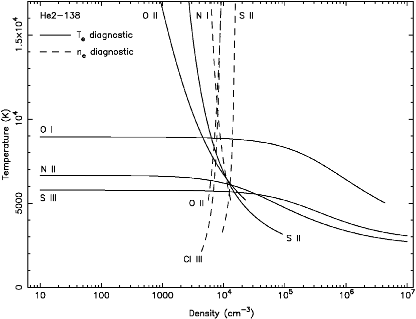
Figure 10.— Diagnostic diagram for He2-138. Dashed lines indicate $n_{e}$ diagnostic curves and solid lines $T_{e}$ diagnostics curves derived from emission line intensities listed in Table 4 input into the ratios listed in Table 6.

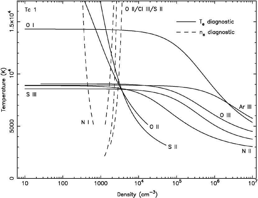
Figure 11.— Diagnostic diagram for Tc 1. Dashed lines indicate $n_{e}$ diagnostic curves and solid lines $T_{e}$ diagnostics curves derived from corresponding emission line intensities listed in Table 4 input into the ratios listed in Table 6.

Emission measures and relative abundances of ions are normally determined from their forbidden line intensities, which have a sensitive dependence upon the kinetic temperature and density of the gas. Electron temperatures $T_{e}$ have been determined for regions of different ionization primarily from the ratio of auroral to nebular line intensities of [O I], [S II], [N II], [O II], [O III], [S III], and [Ar III] using complete radiative and collisional multi-level calculations similar to those in the IRAF nebular package (Shaw & Dufour, 1995), as described by Sharpee et al. (2007) in their study of $s$-process elements in PNe. Similarly, electron densities $n_{e}$ are sensitive to certain line ratios such as [O II] $\lambda$3726/29, [S II] $\lambda$6716/31, [Cl III] $\lambda$5518/38, and [Ar IV] $\lambda$4711/40. We have used all of these forbidden line ratios, when they were observed, and corresponding atomic data listed in Table 5 to calculate appropriate values of $T_{e}$ and $n_{e}$ in Figures 10–12. The resulting values of $T_{e}$ and $n_{e}$ are listed in Table 6 with their formal uncertainties. The densities and temperatures derived from the different lines are generally consistent with each other with the exception of the [N I] for NGC 6543 and Tc1, and the [S II] density for He2-138, as is evident from the plots in Figures 10–12. The disparate densities deduced for He2-138 from the different lines could be real; the result of inhomogeneities. The [N I] lines, on the other hand, are very weak and thus the densities from that doublet are very uncertain.

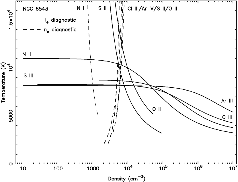
Figure 12.— Diagnostic diagram for NGC 6543. Dashed lines indicate $n_{e}$ diagnostic curves and solid lines $T_{e}$ diagnostics curves derived from corresponding emission line intensities listed in Table 4 input into the ratios listed in Table 6.

In order to properly account for all relevant physical processes when converting the observed emission line flux $F_{c}$ into the emission measure we consider here the full definition of the emission measure. The extinction-corrected flux of an optically thin emission line along a line of sight is

$$F_{c}={\theta_{o}}^{2}[h\nu_{o}/(4\pi)]\int n_{u}A_{ul}\,d\ell\,,$$ (5)

where ${\theta_{o}}^{2}$ is the angular area of the gas being observed, and $A_{ul}$ and $n_{u}$ are the line transition probability and number density of the upper level. The stronger forbidden transitions normally have direct collisional excitation from the ground state as the predominant mechanism exciting the line, therefore it is convenient to write the equation of statistical equilibrium governing the population of the upper level in terms of the ion and electron densities as

$$n_{u}\sum_{k<u}A_{uk}=n_{e}n_{1}q_{1u}(T_{e})[1+\xi(n_{e},T_{e},J_{\nu})]\,,$$ (6)

where $q_{1u}(T_{e})$ is the collision coefficient between the ground state and upper level, and the term $\xi(n_{e},T_{e},J_{\nu})$ represents all other processes contributing to the population of the upper level, e.g., radiative cascading and collisional population from upper levels, collisional de-excitation to lower levels, continuum and resonance fluorescence, and recombination. We formulate the equation this way in order to isolate the term $n_{e}n_{1}$, whose integral along the line of sight is the emission measure of the ion. For the processes listed above, the expression for $\xi$ is

$$\xi(n_{e},T_{e},J_{\nu}) = \left[n_{e}n_{1}q_{1u}\right]^{-1}\left\{\sum_{k>u}n_{k}A_{ku}+n_{e}\sum_{k>1,k\neq u}n_{k}q_{ku}\right.$$ (7)

$$-n_{e}n_{u}\sum_{k\neq u}q_{uk}+\sum_{k\neq u}n_{k}J_{ku}B_{ku}$$

$$\left.-n_{u}\sum_{k\neq u}J_{uk}B_{uk}+n_{e}n_{i+1}\alpha_{u}\right\}\,.$$

Here, $J_{ku}$ and $B_{ku}$ are the mean intensity and Einstein $B$ coefficient for radiative (de-)excitation from level $k$ to level $u$, and $\alpha_{u}$ is the effective recombination coefficient into level $u$.

For most strong forbidden lines direct excitation from the ground states predominates, and $\xi\ll 1$. However, for certain ions, e.g., Fe II and Ni II (Lucy, 1995; Bautista, Peng, & Pradhan, 1996; Bautista & Pradhan, 1996; Bautista, 2004), and certain transitions of CNO (Grandi, 1975) other processes such as radiative excitation and strong coupling between other excited levels contribute to some of the stronger forbidden transitions, such that $\xi>1$ for these lines under certain conditions. The intensities of these lines do not retain a simple linear dependence on $n_{e}n_{1}$, and it is important to treat their excitation via detailed multi-level calculations that involve the radiation field.

We have used detailed calculations of the relevant level populations for all of the ions using the values of $T_{e}$, $n_{e}$, and $J_{\nu}$ appropriate for the level of ionization and augmented by incorporation of additional levels and processes for the ions, to determine the emission coefficients $q_{1u}(Te)$ and $\xi(n_{e},T_{e},J_{\nu})$ for all of the lines listed in Table 4. The radiation fields $J_{\nu}$ for our slit positions have been taken from observations of the central stars by IUE and FUSE for frequencies below the Lyman limit. For frequencies above the Lyman limit we have extrapolated the observed stellar continua by assuming a black body flux at the appropriate temperature for the central stars. The dilution factors at our slit positions were rather small so that radiative excitation by the stellar continua was not competitive in the population of any level that we considered. For Fe II and Ni II we have used the explicit multi-level population processes and cross sections of Bautista, Pradhan, and collaborators to calculate line strengths for these ions. All known processes that might make significant contributions to the line intensities have been included in the above calculations, and corresponding values of $T_{e}$ and $n_{e}$ have been used that are appropriate for the ionization state for each line. Reddening corrected fluxes have then been used to compute ground state emission measures $EM_{i}$ for those ions for which UV absorption was also observed.

Combining equations 5-7 produces the following expression for the emission measure of an ion $i$,

$$EM_{i} \equiv \int n_{e}n_{1}d\ell$$ (8)

$$= 4\pi F_{c}\sum_{k<u}A_{uk}/\left\{h\nu_{o}A_{ul}{\theta_{o}}^{2}q_{1u}(T_{e})\right.$$

$$\times\left.\left[1+\xi(n_{e},T_{e},J_{\nu})\right]\right\}\,.$$

The extinction-corrected fluxes from Table 4, the atomic data and cross sections from the references in Table 5, and the temperatures and densities listed in Table 6 appropriate to the different ions depending upon their level of ionization have all been used to determine the emission measures of ions from equation 8 using the intensities of the various lines for our sample of PNe. The resulting emission measures are presented in Table 7.

5. Comparative Column Densities from Emission and Absorption

5.1. Correction for Different Lines of Sight

Table 7Forbidden Line Emission Measures

Species	$\lambda$(Å)	$EM_{i}$
		(cm-6 pc)
He2-138
C I	8727	00.4040
P II	7875	$<$0.0250
Fe II	5159	00.6100
Ni II	7378	00.0124
O I	6300	12.3600
	6364	13.7900
S II	4069	13.9900
	4076	14.9200
	6716	11.6700
	6731	12.8400
S III	6312	03.9300
	9069	03.8900
NGC 6543
N I	5198	00.0290
	5200	00.0310
O I	6300	00.2270
	6364	00.2340
S II	6716	00.2020
	6731	00.2010
S III	6312	05.4930
	9069	05.5980
Tc 1
O I	6300	00.0600
	6364	00.0730
S II	4069	00.0990
	4076	00.0840
	6716	00.1360
	6731	00.1390
S III	6312	00.7360
	9069	00.9900

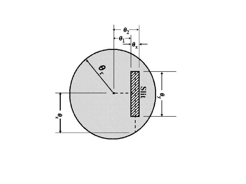
Figure 13.— A schematic indicating the relevant angles discussed in the text that apply the derivations of the volume and shell correction factors $\zeta_{\rm vol}$ and $\zeta_{\rm shell}$, assuming that the nebula is a perfect sphere.

In order to compare directly the results of the absorption and emission abundance analyses the emission measures have to be converted to effective column densities, or vice versa, by dividing the emission measures by the electron density appropriate for each ion. If we designate $<\!\!n_{e}\!\!>_{i}$ as the mean value of $n_{e}$ in the emitting region of the ion $i$, the equivalent emission column density for the ion can be written as

$$N_{em}=EM_{i}/(\zeta<\!\!n_{e}\!\!>_{i})$$ (9)

since the integrals that define the emission measure and the column density of an ion differ only by the factor of the electron density in the emission measure. The constant $\zeta$ is a normalization factor that corrects for the different path lengths along the two lines of sight, viz., our emission line of sight passes through the entire nebula whereas the absorption spectrum line of sight penetrates only to the central star. A derivation of $\zeta$ is given below that allows for the fact that our observations record the flux within a rectangle subtended by the entrance slit of the spectrograph, and this slit is offset from the center of the nebula to avoid contamination of the spectrum by the central star.

A generic representation of our emission-line measurement geometry is shown in Figure 13, with the idealization that the appearance of the nebula is perfectly round in the sky. We consider two fundamentally different simplifications for the distribution of any particular ion within the nebula. The first such representation is a uniformly filled sphere. If the height of the slit $\theta_{y}$ is longer than the chord through the nebula, the volume element $V$ of the sphere that is interior to a projection of the slit with a width equal to $\theta_{x}=\theta_{2}-\theta_{1}$ is given by

$$V={\pi\over 3}~{}\left[\theta_{1}^{3}-\theta_{2}^{3}+3\theta_{r}^{2}\left(\theta_{2}-\theta_{1}\right)\right]~{}.$$ (10)

If we consider that the integration range in equation 5 is over a distance equivalent to the angle subtended by $\theta_{r}$, we can define the correction factor $\zeta_{\rm vol,0}$ to be simply $V$ derived above normalized to the volume within a rectangular box of dimensions $\theta_{x}\theta_{y}\theta_{r}$; hence

$$\zeta_{\rm vol,0}={V\over\theta_{x}\theta_{y}\theta_{r}}={\pi\left[\theta_{1}^{3}-\theta_{2}^{3}+3\theta_{r}^{2}\left(\theta_{2}-\theta_{1}\right)\right]\over 3\theta_{x}\theta_{y}\theta_{r}}~{}.$$ (11)

If $\theta_{y}$ does not subtend the entire chord, we must reduce $\zeta_{\rm vol,0}$ by a factor

$$F_{\rm vol}={1\over\pi}\left[{\theta_{y}\over\theta_{z}}\left(4-{\theta_{y}\over\theta_{z}^{2}}\right)^{\text@frac{1}{2}}+2\sin^{-1}\left({\theta_{y}\over 2\theta_{z}}\right)\right]$$ (12)

where

$$\theta_{z}=\left[\theta_{r}^{2}-\left({\theta_{1}+\theta_{2}\over 2}\right)^{2}\right]^{\text@frac{1}{2}}$$ (13)

is the radius of the circle that represents the intersection of the surface of the sphere with a plane that is aligned with the centerline of the slit. The factor $F_{\rm vol}$ is based on the approximation that $\theta_{x}\ll\theta_{z}$, since it represents the area subtended by lines bounded by $\theta_{y}$ inside the circle relative to the total area of the circle, but only for a circle coincident with the slit centerline. The final value for $\zeta_{\rm vol}$ which applies to a fully filled sphere is given by

$$\zeta_{\rm vol}=F_{\rm vol}\,\zeta_{\rm vol,0}$$ (14)

Our second representation differs from the first in that the material is assumed to be distributed in a thin shell, rather than throughout the entire volume of the nebula. In a development similar to the one that we performed for the volume-filled nebula, we compute the area $A$ of a projection of the slit on the surface of the sphere, under the condition that it is long enough to cover the entire chord,

$$A=2\pi\theta_{r}\left(\theta_{2}-\theta_{1}\right)~{}.$$ (15)

In this case, the normalization box has the dimensions $\theta_{x}\theta_{y}$ multiplied by the thickness of the shell. Since the appropriate path length for equation 5 in this case is the shell thickness, this thickness cancels out in the equation for shell correction factor $\zeta_{\rm shell,0}$, leaving us with the expression

$$\zeta_{\rm shell,0}={A\over\theta_{x}\theta_{y}}={2\pi\theta_{r}\left(\theta_{2}-\theta_{1}\right)\over\theta_{x}\theta_{y}}$$ (16)

The reduction factor $F_{\rm shell}$ for $\theta_{y}<2\theta_{z}$ is given by

$$F_{\rm shell}={2\over\pi}\sin^{-1}\left({\theta_{y}\over 2\theta_{z}}\right)$$ (17)

and this factor reverts to unity for $\theta_{y}\geq 2\theta_{z}$. As before,

$$\zeta_{\rm shell}=F_{\rm shell}\,\zeta_{\rm shell,0}$$ (18)

Values for the angles and correction factors $\zeta_{\rm vol}$ and $\zeta_{\rm shell}$ are given in Table 8, and are based upon nebular diameters taken from the literature, as discussed below. Both values of $\zeta$ for NGC 6543 and Tc 1 are not very far from 2 because the slit heights were only about half the nebular diameters and the slits were positioned rather close to the central stars. The relative change in going from $\zeta_{\rm vol}$ to $\zeta_{\rm shell}$ is large for He2-138 because the slit size was comparable to the nebular diameter, and it was positioned near the nebula’s edge.

The images of He2-138, NGC 6543, and Tc 1 in Figure 6 show that all three PNe possess a degree of spherical symmetry for the overall structure, but also have embedded asymmetrical, inhomogeneous features, e.g., clumps and possible bipolar structure. Differences between the emission and absorption lines of sight therefore depend not just on the footprint of the spectrograph slit on the nebulae and whether the nebulae can be represented as filled shells or thin rings, but also upon small-scale inhomogeneities that lie along one line of sight but not the other. Small-scale structure could well be the dominant cause of differences between the separate lines of sight, and such structure commonly depends on the level of ionization.

Table 8Angles and Correction Factors

	Nebular Identification
Quantity	He2-138	NGC 6543	Tc1
$\theta_{r}$	3.5	9.8	4.8
$\theta_{1}$	2.0	2.0	1.9
$\theta_{2}$	3.5	4.0	3.9
$\theta_{y}$	4.0	10.	4.0
$\zeta_{\rm vol}$	0.985	1.80	1.48
$\zeta_{\rm shell}$	4.12	2.22	2.64

Table 9Comparitive Column Densities from Emission and Absorption Lines

Species	$\log\,N_{abs}$	$EM_{i}$	$<n_{e}>_{i}$	$\log\,N_{em}$	$\log\,N_{abs}-\log\,N_{em}$
	(cm-2)	(cm-6 pc)	(cm-3)	(cm-2)
He2-138 ($\zeta_{\rm vol}=0.985$ $\zeta_{\rm shell}=4.12$)
C I	13.93$\pm 0.16$	00.4040	07000	(14.26, 13.64) $\pm 0.31$	(-0.33, 0.29) $\pm 0.35$
P II	13.58$\pm 0.21$	$<$0.025000	07000	$<$(13.05, 12.43) $\pm 0.42$	$>$(0.53, 1.15) $\pm 0.47$
Fe II	14.37$\pm 0.14$	00.6100	07000	(14.44, 13.82) $\pm 0.64$	(-0.07, 0.55) $\pm 0.66$
Ni II	12.77$\pm 0.17$	00.0124	07000	(12.74, 12.12) $\pm 0.21$	(0.03, 0.65) $\pm 0.27$
O I	$>$15.48$\pm 0.37$	12.8000	07000	(15.76, 15.14) $\pm 0.34$	$>$(-0.28, 0.34) $\pm$0.50
S II	$>$15.49$\pm 0.09$	12.3000	10000	(15.58, 14.96) $\pm 0.26$	$>$(-0.09, 0.53) $\pm 0.28$
S III	15.11$\pm$0.13	03.8900	07500	(15.21, 14.59) $\pm 0.11$	(-0.10, 0.52) $\pm 0.17$
NGC 6543 ($\zeta_{\rm vol}=1.80$ $\zeta_{\rm shell}=2.22$)
O I	13.48$\pm 0.51$	00.2300	05000	(13.89, 13.80) $\pm 0.25$	(-0.41, -0.32) $\pm 0.57$
N I	12.29$\pm 0.25$	00.0300	04000	(13.10, 13.01) $\pm 0.21$	(-0.81, -0.72) $\pm 0.33$
S II	13.64$\pm 0.07$	00.2000	05000	(13.83, 13.74) $\pm 0.14$	(-0.19, -0.10) $\pm 0.16$
S III	15.22$\pm 0.14$	05.5600	05000	(15.27, 15.18) $\pm 0.04$	(-0.05, 0.04) $\pm 0.15$
Tc 1 ($\zeta_{\rm vol}=1.48$ $\zeta_{\rm shell}=2.64$)
O I	13.67$\pm 0.06$	00.0640	02000	(13.82, 13.57)$\pm 0.26$	(-0.15, 0.10) $\pm 0.27$
S II	13.67$\pm 0.09$	00.1370	03000	(13.98, 13.73)$\pm 0.14$	(-0.31, -0.06) $\pm 0.17$
S III	14.93$\pm 0.07$	00.9200	03000	(14.80, 14.55) $\pm 0.04$	(0.13, 0.38) $\pm 0.08$

Our emission spectra provide information on the extent of both large-scale geometrical and small-scale inhomogeneity effects from the intensity variations of the emission lines along the slit length. The slit lengths we used were 4 and 10 arcsec with a spatial resolution of 1 arcsec along the slit, so we have relatively few independent spatial resolution elements. Nevertheless, the range in distance of the slit from the central star over its length is comparable to the offset of the slit center from the central star. Thus, variations of intensity along the slit due to the overall geometry of the nebulae should be comparable to the intensity differences due to the different path lengths of the absorption and emission sightlines. We have measured the variations in intensity of the [S III] and [O I] lines, representing our highest and lowest ionization species, along the slit in the three PNe. We find for Tc 1 that both the [S III] and [O I] lines have a very uniform distribution of intensity throughout the full slit, and with no measurable differences between the two slit positions. Thus, for Tc 1 the measurements indicate that the emission and absorption lines of sight are likely to be very similar.

For He2-138 the [S III] and [O I] lines have virtually identical, smooth intensity distributions where the intensity peaks at the center and decreases outward toward the ends of the slit where it falls off rapidly near the ends. The intensity profile is more characteristic of a filled volume than a thin shell distribution of gas, but the smaller size of this nebula causes it to fill only 3 arcsec of the 4 arcsec slit length so the geometrical factor zeta represents an important correction for this object. Since there is no indication of differences in the spatial distribution of the ions based on their ionization level the geometrical normalization factor zeta is the same for all of the lines. The fact that the emission spectra sampled the outer edge of the nebula makes the corresponding geometrical correction for this PN rather uncertain, as was explained in §4.1.1. Thus, we consider the results for He2-138 to be less reliable than those of Tc 1 and NGC 6543.

NGC 6543 presents a more complicated picture in terms of the differences between the two lines of sight. The [S III] completely fills the slits with a uniform intensity for one of the slit positions, but shows variations of $\sim$25 percent in the other position. The [O I] completely fills the slits also, but shows large variations along the slit near the center. Thus, the lowest ionization species in this PN display a pronounced small-scale structure that may cause the emission and absorption lines of sight to be quite different for the lowest ionization lines. Based on the intensity variations one must admit the possibility of differences in the column densities along different lines of sight for the neutral species to be as large as factors of 3 for this object - an uncertainty that compromises its usefulness for the neutral species [O I] and [N I].

If the stellar absorption and nebular emission spectroscopy are obtained at sufficiently high resolution one can use radial velocity information from resolved line profiles to match velocity components of optical emission with the corresponding UV absorption produced in the same velocity intervals. A comparison of these quantities within the same velocity interval of the gas provides a more accurate assessment of the comparative abundances than comparing the total emission measure and column density integrated over the full profiles. Local values of the emission column density can be determined for specific kinematic regions within the nebulae. Averaging these values over the full velocity range for the nebular shell will produce the global emission column density for the ion, and also information on its fluctuations as a function of velocity. Since thermal and expansion velocities of nebulae are of order 10–20 km s^-1 a spectral resolution less than 10 km s^-1 is optimal to perform the analysis this way. Our emission spectra lack the necessary spectral resolution to perform such an analysis, and therefore we work with the integrated (over wavelength) emission measures and column densities.

5.2. Comparison of Absorption & Emission Column Densities

The absorption column densities obtained from UV resonance lines refer specifically to those ions occupying the lower level of the transition. In order to obtain the total column density of the ion the column densities for all the individual fine-structure levels of the ground state must be summed together. In our STIS spectra some ions had blended absorption profiles for one or more of the transitions from the ground state fine-structure levels that prevented us from deriving the column densities for those levels. We have determined the column densities of ions in those levels by taking values of $T_{e}$ and $n_{e}$ obtained from the emission lines for that ion to solve for the level populations relative to the levels for which column densities were determined. Additionally, when more than one resonance multiplet of an ion has yielded a column density we have computed the mean value for the ion by weighting individual values according to the inverse square of their uncertainties. These calculations, which have been applied to the absorption column densities in Table 3, yield the total ion column densities, $N_{abs}$, to the central star, and these are listed in Table 9 together with the formal errors that result from the quantifiable uncertainties that are discussed below.

Emission measures for the same ions that have been observed in absorption, and which appear in Table 7 for our sample of PNe, are also presented in Table 9. For ions where more than one forbidden line yields an emission measure we have determined the average of the values, with stronger weight being given to the lines of higher intensity and lower Boltzmann factor. Using the corresponding values of the electron density for each of the ions the resulting emission column densities, $N_{em}$, have been determined from the emission measures from equation 9. These are given in the penultimate column of Table 9 together with the combined errors, having been normalized to the absorption path length by dividing by the geometrical factor $\zeta$.

A comparison of the values of $N_{abs}$ and $N_{em}$ for the different ions from the two completely independent abundance analyses shows moderately good agreement, with the exceptions of P II in He2-138 and N I in NGC  6543. Absolute abundances determined from the forbidden emission lines and UV absorption lines give the same results within $\pm$0.3 dex for adjacent lines of sight, which is comparable to the combined formal errors of the analyses. The 1$\sigma$ errors in the column densities derived from the analyses represent the uncertainties that are quantifiable. There are also systematic errors that arise from assumptions rather than measurement uncertainties, and both sources of error affect the accuracy of our comparison of forbidden and recombination line column densities.

The primary sources of error for the absorption column densities are (a) the determination of the proper continuum level, (b) the low S/N of the intensities of weak absorption lines, (c) the insensitivity of intensity to column density for saturated lines, and (d) the determination of total ground state column density for states with fine-structure levels when absorption from one or more of the levels is either not observed or saturated. The main sources of error for the emission column densities are uncertainties in (a) the flux calibration of the echelle spectra, which are at the 5–10 percent level, (b) collision strengths for some of the forbidden lines, and (c) the correct values of $T_{e}$ and $n_{e}$ that correspond to each of the transitions, as assigned to the various ions from the diagnostics shown in Figures 10–12. The atomic data for most of the forbidden lines that we have used for diagnostics and the determination of column densities are believed to be known to better than 30 percent accuracy. With the exception of the [P II] line the current values for most of the forbidden line collision strengths and transition probabilities are the result of calculations by independent methods over the past three decades that have converged on values that are in good agreement with each other and that have changed little over the past five years. Thus, the atomic data are not likely to be major sources of error. Rather, the largest sources of formal errors in the emission column densities are uncertainties in the values of temperature and density. Because line intensities depend upon these two parameters, errors in $T_{e}$ and $n_{e}$ translate to errors in the column density. Most of the lines are in the low density limit and therefore the emission measures are rather insensitive to density. However, because of the Boltzmann factor the line intensities are sensitive to $T_{e}$. The errors caused by uncertainties in the temperature, together with uncertainties in intensity measurement and flux calibration, form the basis for the combined error that is presented in Table 9 for each emission column density. To these uncertainties must be added the unknown errors in collision strengths and those differences that small-scale inhomogeneities may cause between the lines of sight.

Several features of Table 9 merit comment. First, due to a combination of weak, saturated, or strongly blended UV absorption lines coupled with the failure of our nebular spectra to detect forbidden lines from some ions, there are relatively few ions for which we were able to derive independent abundances from both UV absorption and forbidden emission lines. Even with the relatively long slit used to sample substantial portions of the PNe shells we were not successful in detecting weak emission lines from a number of the ions for which column densities had been measured from the STIS spectra.

Second, with the exception of S⁺² all of the ion species listed in Tables 7 and 9 are the lowest ionization stages that have ionization potentials greater than 13.6 eV. This means that some fraction of most of the ions we have measured could exist in cold, neutral gas residing either within dense clumps embedded inside the nebula or in a foreground shell of material around the nebula. Such gas would complicate our analysis by increasing the absorption column density without having any effect on the emission lines, leading to legitimate differences between the emission and absorption column densities. Fortunately, we can test for this possibility by comparing $N_{abs}$(O I) with $N_{abs}$(S II). The ionization fraction of O is closely coupled to that of H through a charge exchange reaction that has a large rate constant (Field & Steigman, 1971; Chambaud et al., 1980), which guarantees that the amount of O I in the ionized gas is quite low and that practically all of the O is neutral in H I gas. By contrast, in an H II region a reasonable fraction of the S will be in the form of S⁺ since its ionization potential is high (23.3 eV). Furthermore, in an H I region nearly all of the S should also be singly ionized. Therefore, from H I gas we expect to find the ratio $N_{abs}$(O I)/$N_{abs}$(S II) to be approximately equal to the solar value of [O/S] = 1.46, assuming that neither of the elements are significantly condensed onto dust grains nor are they enriched or depleted by nuclear processes within the AGB progenitor of the central star. A ratio smaller than this value signifies progressively less contribution to the column densities from neutral gas.

For Tc 1 we have found that $N_{abs}$(O I)$\approx$$N_{abs}$(S II), which indicates that any contribution from neutral material must be so small that it can be neglected for our study. The situation for NGC 6543 is not quite so straightforward because our inferred value of $N_{abs}$(O I) for the nebula is based on the marginal detection of O I*. Our ability to directly measure O I in the ground fine-structure level is compromised by possible P II $\lambda$1301.87 absorption from foreground ISM gas at a velocity v = -14 km s^-1, which appears at the same wavelength as the velocity-shifted O I $\lambda$1302.17 line from the nebular shell. Nevertheless, we can derive an upper limit to the O I column density for the nebula from this feature, which has equivalent width $EW=10$ mÅ, by assuming the foreground P II absorption to be negligible. When we do this, we derive a value $\log N$(O I) = 13.2, an amount that is above the lower bound for our calculated $\log$ $N_{abs}$(O I) that is listed in Table 9. However, this value is still substantially lower than our measurement of $N_{abs}$(S II), so once again we are assured that contamination of the column densities from neutral gas is negligible for NGC 6543.

We are unable to make any assertion about $N_{abs}$(O I)/$N_{abs}$(S II) toward He2-138 because both column densities were recorded as lower limits (the lines are strongly saturated; see footnote c in Table 3). However, in the spectrum of the central star for this nebula we see absorption features from excited H₂ at v = -62 km s^-1, which is a strong indication that we are viewing a photodissociation region at the inner edge of a neutral shell surrounding the nebula. Thus, it is possible for this one object that $N_{abs}$ for ions that can exist within H I regions could add to the contributions from the ionized nebula. This may explain why $N_{abs}$(P II)$\gg$$N_{em}$(P II) for this PN, although it is then puzzling why the discrepancies for Fe II and Ni II are not nearly as large unless both of them are condensed onto grains.

Finally, we point out that heavy element recombination lines for the ion species that we studied by UV absorption, and which are substantially weaker than the forbidden lines, remained under the detection threshold of our spectra. This limits our ability to make a direct comparison of abundances determined from recombination lines for our PNe. However, although our spectra did not detect recombination lines originating from any of the ions in Tables 7 and 9 from which UV resonance absorption was observed, we did observe C II, N II, and O II recombination lines. Any information that can be obtained from an analysis of these recombination lines is potentially useful. Of the above ions only the O II recombination lines originate from a parent ion for which forbidden lines were observed, viz., O⁺², so the column densities inferred from these lines are considered in the following section.

5.3. Recombination Line Column Densities

The results of Table 9 show that the absorption and forbidden emission column densities agree within the uncertainties of measurement error, inaccuracies in the values of temperature and density, and inhomogeneities that cause the adjacent lines of sight to sample different components of the nebulae. This agreement indicates that nebular analyses based upon forbidden emission lines yield heavy element abundances that are the same as those derived from absorption lines-the key result from this study. That said, what conclusions can be drawn from our sample of PNe about nebular abundances based on recombination lines? Do our objects show the same discrepancies exhibited by other PNe?

Table 10Recombination Line Abundances

Line(Multiplet)	$F$	ADF
	(erg cm-2 s-1)
NGC 6543
O II $\lambda$4069.62,.88 (10)	5.52(-14)	2.24
$\lambda$4072.15 (10)	4.32(-14)	1.88
$\lambda$4110.79 (20)	1.16(-14)	5.01
$\lambda$4153.30 (19)	2.72(-14)	3.61
$\lambda$4317.14 (2)	2.10(-14)	2.59
$\lambda$4345.56 (2)	2.47(-14)	3.28
$\lambda$4349.43 (2)	2.85(-14)	1.57
$\lambda$4638.86 (1)	2.91(-14)	2.59
$\lambda$4641.81 (1)	7.34(-14)	2.87
$\lambda$4649.14 (1)	8.59(-14)	1.75
$\lambda$4650.84 (1)	3.27(-14)	3.21
$\lambda$4661.63 (1)	3.20(-14)	2.47
Average		2.8$\pm 0.9$
Tc 1
O II $\lambda$4069.62,.88 (10)	4.75(-16)	1.97
$\lambda$4072.15 (10)	4.26(-16)	1.82
$\lambda$4153.30 (19)	1.58(-16)	2.12
$\lambda$4317.14 (2)	2.11(-16)	2.88
$\lambda$4345.56 (2)	2.93(-16)	4.09
$\lambda$4349.43 (2)	2.98(-16)	1.66
$\lambda$4641.81 (1)	7.08(-16)	2.72
$\lambda$4650.84 (1)	3.73(-16)	3.48
$\lambda$4661.63 (1)	4.37(-16)	3.18
Average		2.5$\pm 0.9$

We have detected a number of the same O II recombination lines from NGC 6543 and Tc 1 that have been studied extensively in PNe over the past decade and used to determine relative O⁺² abundances (Liu et al., 2000; Robertson-Tessi & Garnett, 2005). Since the [O III] forbidden lines are strong in both objects it is straightforward to determine the abundance of O⁺² as derived from the two types of lines. No recombination lines were observed in the spectrum of the very low ionization nebula He2-138.

The permitted O II lines from multiplets 1, 2, 10, 19, and 20 have been shown to be populated by recombination and to yield, among themselves, consistent values of the O⁺² abundance in H II regions and PNe (Tsamis et al., 2003; Wesson, Liu, & Barlow, 2005). We have used the extinction-corrected intensities of these lines, the observed intensities of which are shown in Table 10, to compute the O⁺² abundance relative to that determined from the [O III] $\lambda\lambda$5007, 4959 lines. This ratio is referred to as the “abundance discrepancy factor” (ADF), and for PNe and H II regions always has values that are greater than unity. Using the same cross sections and procedures described by Robertson-Tessi & Garnett (2005) and Wesson, Liu, & Barlow (2005), we have determined ADF values from the individual O II lines, and these are listed in the last column of Table 10. The resulting mean values of the ADFs for NGC 6543 and Tc 1 are 2.8 and 2.5 (0.45 and 0.40 dex), respectively. The mean ADF of 2.8 found here for NGC 6543 is consistent with the previous determinations of ADF = 3.0 and 3.8 from other lines of sight through this same nebula (Kingsburgh, Lopez, & Peimbert, 1996; Wesson & Liu, 2004). Thus, at least two of our objects show the same discrepancies between the recombination and forbidden line abundances for O⁺² that are typical of PNe, and we have not by chance studied nebulae for which the ADFs are close to unity.

Since there is good agreement between the absorption and forbidden line column densities in our objects, one can infer from the above results that recombination lines are likely to produce emission column densities that are significantly higher than those derived from absorption lines. The final column of Table 9 shows that the mean of the forbidden emission line column densities is marginally larger than that of the absorption column densities for each of the PNe. The recombination line column densities would produce a larger discrepancy. However, because the ADFs for NGC 6543 and Tc 1 are of the same size as the uncertainties in the column densities, a larger sample of PNe is needed, especially including some objects with relatively large ADFs, before a definitive statement can be made that recombination abundances are not correct. Given that we do not detect any recombination lines from parent ions for which we measured UV absorption lines, a direct comparison of absorption and recombination line column densities for the same ions is likely to remain elusive. Realistically, the only ions in Tables 7 and 9 that are likely to be parent ions of detectable recombination lines are S⁺ and S⁺². With deeper spectra it should be possible to observe the S II recombination lines in our PNe, however the relevant recombination coefficients are not known and are very difficult to calculate with any accuracy (P. Storey, private communication).

Emission line analysis of a large number of PNe has shown that recombination lines originating from C⁺², N⁺², O⁺², and Ne⁺² ions all yield roughly the same relative abundances among themselves as do the collisionally excited forbidden and intercombination lines from these same ions, and that the recombination lines consistently indicate higher abundances with respect to H and He (Robertson-Tessi & Garnett, 2005; Wesson, Liu, & Barlow, 2005; Liu et al., 2006). The discrepancies do not appear to arise from problems with the atomic data, rather they seem to be linked to characteristics that are specific to the nebulae. Thus, the ADFs for doubly ionized CNONe tend to be approximately the same in individual objects, and they vary in step with each other from one nebula to the next although there are exceptions to this rule, e.g., NGC 6720 (Garnett & Dinerstein, 2001).

If the agreement among the CNONe ADFs also applied to S⁺² one could use the ADFs we have derived from the O II lines in NGC 6543 and Tc 1 to infer the recombination line column density for S⁺², based on the [S III] emission measure. However, the ADFs for elements in the 3rd row of the periodic table, including sulfur, are virtually unknown because so few recombination lines are detected and the relevant cross sections are not known (Barlow et al., 2003). The only 3rd row ion for which a recombination abundance has been determined is Mg⁺², from Mg II lines having been measured in ten PNe by Barlow et al. (2003). They found the Mg⁺²/H⁺ abundances for their objects to show little evidence for enhancement over the solar value, contrary to the large O⁺²/H⁺ enhancements derived from the O II recombination lines in the same PNe. They conclude that the recombination line abundance discrepancies may be a phenomenon restricted to ions of the 2nd row of the periodic table, viz., C, N, O, and Ne, and not exhibited by 3rd row ions.

Our current study shows nonetheless that the electron densities and temperatures deduced from the usual forbidden line analysis are correct over a range of ionization zones that should include the regions where C⁺², N⁺², O⁺², and Ne⁺² reside. This means that the large ADFs for the second row elements cannot be reflecting errors in the forbidden line abundances due to the use of incorrect values of $n_{e}$ or $T_{e}$. It would be necessary to find another mechanism that would affect the forbidden line abundances derived for C⁺², N⁺², O⁺², and Ne⁺², but not those found for S⁺ and S⁺². In our opinion this makes factors affecting the recombination line abundances almost certainly the cause of the abundance discrepancies.

6. Summary

The results reported here are derived from a limited sample of PNe and are based upon observations that may not be extended in the near future unless STIS is repaired and put back into service on HST. For this sample we find that the forbidden lines yield absolute abundances for C I, Fe II, Ni II, O I, S II, and S III that are consistent with those derived from their absorption lines along adjacent sight lines. Within the uncertainties in the line intensities and calculations, the good agreement between the column densities derived from the forbidden emission lines and the UV absorption lines for the three PNe represents a validation of both types of analysis. It strengthens confidence in the abundances derived from forbidden emission lines in spite of discrepancies with the abundances derived from high level permitted recombination lines from the same ions, and is the primary result of this investigation.

Although recombination lines were detected in only two of the three objects in this study, those two PNe do show factor 2.5–-2.8 discrepancies between the O⁺² abundances derived from forbidden lines and those from recombination lines. This demonstrates that we have studied PNe in which the abundance discrepancy problem exists. Not being able to independently measure an abundance for O⁺² from its UV resonance lines, which fall outside of the HST wavelength range, we cannot confirm that the recombination abundances for O⁺² are anomalously high. Nor can we use the similarity in the abundance discrepancy factors of C⁺², N⁺², and Ne⁺² with that of O⁺² to make a comparison of the inferred recombination abundances of these ions with those from an absorption analysis because their UV resonance lines also fall outside of the HST wavelength range. The one doubly ionized ion for which we do have good absorption data, S⁺², did not have recombination lines detected in our nebular spectra.

We have shown that the electron densities and temperatures deduced for a wide range of ionization levels do give correct abundances using the forbidden lines from ions of other elements within the same ionization zone as O⁺² (and C⁺², N⁺², and Ne⁺²). In particular, the forbidden line abundances for S⁺² are in good agreement with the absorption line abundances for S⁺². This is an important constraint since any explanation of the ADF for O⁺² and other second row elements that implicates errors in the forbidden line abundances would have to invoke a mechanism that does not affect the forbidden line abundances of other ions such as S⁺² in the same ionization zone.

RW, EBJ, and JAB gratefully acknowledge support for this research from data reduction grant HST-GO-09736-A from STScI. JAB and EP also acknowledge financial support from NSF through grant AST-0305833. Special thanks are due Jessica Kim and Paul Goudfrooij for their skillful restitution of a STIS spectrum that was anomalous.

References

- Acker et al. (1992) Acker, A., Ochsenbein, F., Stenholm, B., Tylenda, R., Marcout, J., & Schohn, C. 1992, Strasbourg- ESO Catalogue of Galactic Planetary Nebulae (Garching: ESO)
- Aggarwal (1983) Aggarwal, K.M. 1983, ApJS, 52, 387
- Aggarwal, Baluja, & Tully (1982) Aggarwal, K.M., Baluja, K.L., & Tully, J.A. 1982, MNRAS, 201, 923
- Baluja & Zeippen (1988) Baluja, K.L. & Zeippen, C.J. 1988, J. Phys. B, 21, 1455