Hamiltonian approach to geodesic image matching

Abstract.

This paper presents a generalization to image matching of the Hamiltonian approach for planar curve matching developed in the context of group of diffeomorphisms. We propose an efficient framework to deal with discontinuous images in any dimension, for example 2D or 3D. In this context, we give the structure of the initial momentum (which happens to be decomposed in a smooth part and a singular part) thanks to a derivation lemma interesting in itself. The second part develops a Hamiltonian interpretation of the variational problem, derived from the optimal control theory point of view.

1. Introduction

This paper arose from the attempt to develop the multi-modal image matching in the framework of large deformation diffeomorphisms. Initiated by the work of Grenander, this context was deeply used since [Tro95], especially with applications to computational anatomy. The method followed is the classical minization of an energy on the space of diffeomorphisms, which enables to compute geodesics on this space and to derive the evolution equations. In most of the papers, the group of diffeomorphisms acts on the support of the template; we add to this one a diffeomorphisms group action on the level set of the template. This action is a natural way to cope with the multi-modal matching and could be, in a certain way, compared to the metamorphoses approach exposed in [TY05]: the metamorphoses are another way to act on the images but the goal is very different in our case. Matching in our context, is to find a couple $(\eta,\phi)$ which minimizes the energy

$$E(\eta,\phi)=D(Id,(\eta,\phi))^{2}+\frac{1}{\sigma^{2}}\|\eta\circ I_{0}\circ\phi^{-1}-I_{targ}\|_{L^{2}}^{2},$$ (1)

with $I_{0}$ the initial function (or image) and $I_{targ}$ the target function, Id is the identity map in the product of groups, $\sigma$ is a calibration parameter. The distance $D$ is obtained through a product of Riemannian metrics on the diffeomorphisms groups.
All the complexity is then carried by the group of diffeomorphisms and its action: in the particular case of landmark matching, the geodesics are well described. The problem is reduced in this case to understand the geodesic flow on a finite dimensional Riemannian manifold. It should be also emphasized that this problem can be seen as an optimal control problem. In [BMTY05], numerical implementation of gradient based methods are strongly developed through a semi-Lagrangian method for computing the geodesics. A Hamiltonian formulation can be adopted to provide efficient applications and computations through the use of the conservation of momenta. In [VMTY04], statistics are done on the initial momenta which is a relative signature of the target functions. The existence of geodesics from an initial momentum was deeply developed in [TY05], but this work dealt only with smooth functions for $I_{0}$ (essentially $H^{1}$) however with a very large class of momenta. An attempt to understand the structure of the momentum for an initial discontinuous function was done in the matching of planar curves in [GTL06].
We propose thereafter a framework to treat discontinuous functions in any dimension: the main point is to derive the energy function in this context.
Finally, we chose to give a Hamiltonian interpretation of the equations which is the proper way to handle the conservation of momentum. This formulation includes the work done in [GTL06] but does not capture the landmark matching. The formulation we adopt gives a weak sense to the equations and we prove existence and uniqueness for the weak Hamiltonian equations within a large set of initial data. A word on the structure of initial data: the article on planar matching ([GTL06]) focuses on Jordan curves. The main result is the existence for all time and uniqueness of Hamiltonian flow. The initial data are roughly a Jordan curve for the position variable and a vector field on this curve for the momentum. In our context, we choose four variables $(I_{0},\Sigma_{0},p_{0},P_{0})$. $I_{0}$ is the initial function with a set of dicontinuities $\Sigma_{0}$, $p_{0}$ is the momentum on the set $\Sigma_{0}$ and $P_{0}$ is the momentum for the smooth part of the initial function. This is a natural way to understand the problem and the choice to keep the set of discontinuity as a position variable can lead to larger applications than only choose $I_{0}$ as position variable.

The paper is organized as follows. We start with a presentation of the framework underlying equation (1). We present a key lemma concerning the data attachment term with respect to the $\eta$ and $\phi$ variables. Its proof is postponed to the last section. Then we derive the geodesics equations and ensure the existence of a solution for all time from an initial momentum. In the second part of this paper, we give the weak formulation of the Hamiltonian equations, and deal with the existence and uniqueness for this Hamiltonian formulation.

2. Framework and notations

2.1. The space of discontinuous images

Let $n\geq 1$ and $M\subset\mathbb{R}^{n}$ a $C^{1}$ bounded open set diffeomorphic to the unit ball.
We denote by $BV(M)$ the set of functions of bounded variation. The reader is not supposed to have a broad knowledge of $BV$ functions. Below, we restrict ourselves to a subset of $BV$ functions which does not require the technical material of $BV$ functions. However it is the most natural way to introduce our framework. Recall a definition of $BV$ functions:

Definition 1.

A function $f\in L^{1}(M)$ has bounded variation in $M$ if

$$\sup\{\int_{M}f\;\mathrm{div}\phi\;dx\;|\;\phi\in C_{c}^{1}(M,\mathbb{R}^{n}),|\phi|_{\infty}\leq 1\}<\infty.$$

In this case, $Df$ is defined by $\int_{M}f\;\mathrm{div}\phi\;dx=-\int_{M}Df\;\phi\;dx$.

Definition 2.

We define $\text{Im}(M)\subset BV(M)$ such that for each function $f\in\text{Im}(M)$, there exists a partition of $M$ in Lipschitz domains $(U_{i})_{i\in[0,k]}$ for an integer $k\geq 0$, and the restriction $f_{|U_{i}}$ is Lipschitz .

Remark 1.

The extension theorem of Lipschitz function in $\mathbb{R}^{n}$ enables us to consider that on each $U_{i}$, $f_{|U_{i}}$ is the restriction of a Lipschitz function defined on $\mathbb{R}^{n}$.

On the definition of a Lipschitz domain $U$: we use here (to shorten the previous definition) a large acceptation of Lipschitz domains which can be found in chapter 2 of [DZ01]. Namely, $U$ is a lip domain if there exists a Lipschitz open set $\Omega$ such that $\Omega\subset U\subset\bar{\Omega}$. In the proof of the derivation lemma 7, we give the classical definition of Lipschitz open set that we use above. In a nutshell, an open set is Lipschitz if for every point of the boundary there exists an affine basis of $\mathbb{R}^{n}$ in which we can describe the boundary of the open set as the graph of a Lipschitz function on $\mathbb{R}^{n-1}$. We chose to deal with Lipschitz domains because it makes sense in the context of application to images.

Example 1.

The most simple example is a piecewise constant function, $f=\sum_{i=1}^{k}a_{i}\mathbf{1}_{U_{i}}$ with $a_{i}\in\mathbb{R}$.

Remark 2.

Our framework does not allow us to treat the discontinuities along a cusp, but we can deal with the corners respecting the Lipschitz condition.

Let $f\in\text{Im}(M)$, we denote by $J_{f}$ the set of the jump part of $f$. As a $BV(M)$ function, we can write the distributional derivative of $f$: $Df=\nabla f+D^{c}f+j(f)(x)\mathcal{H}^{n-1}\llcorner J_{f}$. $\nabla f$ is the absolutely continuous part of the distributional derivative with respect to the Lebesgue measure and $D_{c}$ is the Cantor part of the derivative. In other words, with the classical notations $j(f)(x)=(f^{+}(x)-f^{-}(x))\nu_{f}(x)$, where $(f^{+},f^{-},\nu_{f}):J_{f}\mapsto\mathbb{R}^{n}\times\mathbb{R}^{n}\times\mathbf{S}^{n-1}$ is a Borel function. The functions $f^{+}$ and $f^{-}$ are respectively defined as $f^{+}(x)=\lim_{t\mapsto 0^{+}}f(x+t\nu_{f}(x))$ and $f^{-}(x)=\lim_{t\mapsto 0^{-}}f(x+t\nu_{f}(x))$. Naturally, $j(f)$ does not depend on the choice of the representation of $\nu_{f}$, in fact $j(f)$ is homogeneous to the gradient. See for reference [Bra98] or [AFP00]. In our case, the Cantor part is null from the definition.
We then write for $f\in\text{Im}(M)$,

$$Df=\nabla f+j(f)(x)\mathcal{H}^{n-1}\llcorner J_{f}.$$ (2)

2.2. The space of deformations

We denote by $V_{M},<,>_{V}$ a Hilbert space of square integrable vector fields on $M$, which can be continuously injected in $(\chi_{0}^{p}(M),\|.\|_{p,\infty})$, the vector space of $C^{p}$ with $p\geq 1$ vector fields which vanish on $\partial M$. Hence, there exists a constant $c_{V}$ such that for all $v\in V$:

$$\|v\|_{p,\infty}\leq c_{V}\|v\|_{V}.$$

Hence this Hilbert space is also a RKHS (Reproducing Kernel Hilbert Space), and we denote by $k_{V}(x,.)\alpha$ the unique element of $H$ which verifies for all $v\in H$: $<v(x),\alpha>=<k_{V}(x,.)\alpha,v>_{H}$, where $<,>$ is the euclidean scalar product and $\alpha$ a vector in $\mathbb{R}^{n}$. This will enable an action on the support $M$.

We denote by $S,<,>_{S}$ a Hilbert space of square integrable vector fields on $\mathbb{R}$, as above. We denote by $k_{S}(x,.)$ its reproducing kernel. This will enable the action on the level set of the functions.

Through the following paragraph, we recall the well-known properties on the flow of such vector fields and its control. Most of them can be found in chapter $2$ of [Gla05], and are elementary applications of Gronwall inequalities. (See Appendix B in [Eva98])

Let $v\in L^{2}([0,1],V)$, then with [Tro95] the flow is defined:

$$\partial_{t}\phi_{0,t}^{v} = v_{t}\circ\phi_{0,t}^{v},$$ (3)

$$\phi_{0} = Id.$$ (4)

For all time $t\in[0,1]$, $\phi_{0,t}^{v}$ is a $C^{1}$ diffeomorphism of $M$ and the application $t\mapsto d_{x}\phi_{0,t}^{v}$ is continuous and solution of the equation:

$$d_{x}\phi_{0,t}^{v}=Id+\int_{0}^{t}d_{\phi_{0,s}^{v}(x)}v_{s}.d_{x}\phi_{s}^{v}ds.$$ (5)

We dispose of the following controls, with respect to the vector fields; let $u$ and $v$ be two vector fields in $\in L^{2}([0,1],V)$ and $T\leq 1$:

$$\|\phi^{u}_{0,t}-\phi^{v}_{0,t}\|_{\infty} \leq c_{V}\|v-u\|_{L^{1}[0,T]}\exp(c_{V}\|v\|_{L^{1}[0,T]}),$$ (6)

$$\|d\phi^{u}_{0,t}-d\phi^{v}_{0,t}\|_{\infty} \leq 2c_{V}\|v-u\|_{L^{1}[0,T]}\exp(c_{V}\|v\|_{L^{1}[0,T]}).$$ (7)

And we have controls with respect to the time, with $[s,t]\subset[0,T]$:

$$\|\phi_{0,t}^{v}-\phi_{0,s}^{v}\|_{\infty} \leq \int_{s}^{t}\|v_{r}\|_{\infty}dr\leq c_{V}\int_{s}^{t}\|v_{r}\|_{V}dr,$$ (8)

$$\|\phi_{0,t}^{v}-\phi_{0,s}^{v}\|_{\infty} \leq c_{V}\sqrt{|s-t|}\|v\|_{L^{2}},$$ (9)

$$\|d\phi_{0,t}^{v}-d\phi_{0,s}^{v}\|_{\infty} \leq C\exp(C^{\prime}\sqrt{T}\|v\|_{L^{2}[0,T]})\int_{s}^{t}\|v_{r}\|_{V}dr.$$ (10)

with the constants $C$ and $C^{\prime}$ depending only on $c_{V}$. Obviously these results are valid if $S$ replaces $V$. In this case, we write $\eta_{0,t}$ for the flow generated by $s_{t}$. With the group relation for the flow, $\eta_{t,u}\circ\eta_{s,t}=\eta_{s,u}$.

The group we consider is the product group of all the diffeomorphisms we can obtain through the flow of $u\in L^{2}([0,1],V\times S)$.

We aim to minimize the following quantity, with $\mu$ the Lebesgue measure:

$$\mathcal{J}(v_{t},s_{t})=\frac{\lambda}{2}\int_{0}^{1}\|v_{t}\|_{V}^{2}dt+\frac{\beta}{2}\int_{0}^{1}\|s_{t}\|_{S}^{2}dt+\int_{M}|\eta_{0,1}\circ I_{0}\circ\phi_{0,1}^{-1}(u)-I_{targ}(u)|^{2}d\mu(u),$$ (11)

with $\eta_{0,t}$ the flow associated to $s_{t}$. Remark that the metric we place on the product groups $V\times S$ is the product of the metric on each group which is represented by the first two terms in (11). The functions $I_{0},I_{targ}$ lie in $\text{Im}(M)$. In one section below, we prove classically that there exists at least one solution and we derive the geodesic equations which give the form of the initial momentum.

3. Derivation lemma

This derivation lemma may be useful in many situations where discontinuities arise. Consider for exemple two Lipschitz open sets $U$ and $V$. One may want to deform one of these open sets while the second remains unchanged (figure below). The basic case is the following:

$$J_{t}=\int_{V}\chi_{U}\circ\phi_{t}^{-1}dx=\mu(V\cap\phi_{t}(U)),$$

with $\mu$ the Lebesgue measure. We answer to the differentiation of $J_{t}$, we obtain a sort of Stokes formula with a perturbation term. We discuss below a more general formula to apply in our context. The final result is the proposition 1:

Lemma 1.

Let $U,V$ two bounded Lipschitz domains of $\mathbf{R}^{n}$. Let $X$ a Lipschitz vector field on $\mathbb{R}^{n}$ and $\phi_{t}$ the associated flow. Finally, let $g$ and $f$ Lipschitz real functions on $\mathbf{R}^{n}$. Consider the following quantity depending on $t$,

$$J_{t}=\int_{\phi_{t}(U)}f\circ\phi_{t}^{-1}g\mathbf{1}_{V}d\mu,$$

where $d\mu$ is the Lebesgue measure, then

$$\partial_{t|t=0^{+}}J_{t}=\int_{U}-<\nabla f,X>g\mathbf{1}_{V}d\mu+\int_{\partial U}<X,n>fg\tilde{\mathbf{1}}_{V}(X)d\mu_{|\partial U}.$$ (12)

with $\tilde{\mathbf{1}}_{V}(X)(y)=\lim_{\epsilon\mapsto 0^{+}}\mathbf{1}_{\bar{V}}(y+\epsilon X)$, if the limit exists, $0$ elsewhere. And we denote by $d\mu_{|\partial U}$ the measure on $\partial U$ and $n$ the outer unit normal.

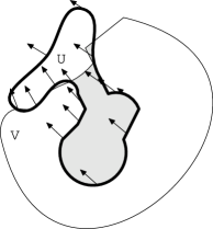
Figure 1. Evolution of the area between two Lipschitz curves. (The arrows represent $X$ along the boundary of $U$)

As a corollary, we deduce:

Corollary 1.

We have,

$$\partial_{t|t=0^{+}}\mu(V\cap\phi_{t}(U))=\int_{\partial U}<X,n>\tilde{\mathbf{1}}_{V}(X)d\mu_{|\partial U},$$

with $\tilde{\mathbf{1}}_{V}(X)(y)=\lim_{\epsilon\mapsto 0^{+}}\mathbf{1}_{\bar{V}}(y+\epsilon X)$, if the limit exists, $0$ elsewhere. And we denote by $d\mu_{|\partial U}$ the measure on $\partial U$ and $n$ the outer unit normal.

In this case, the derivation formula is a Stokes’ formula in which one takes only into account the deformation viewed in $V$.

Below is a figure to illustrate the lemma:

Remark 3.

We could generalize the lemma to finite intersection of Lipschitz domains, with the same scheme of the proof developed above. We gain hence generality which seems to be very natural for concrete applications.

This generalization for Lipschitz domains is sufficient for the application we aim, and this application is presented in the paragraph below to derive the geodesic equations. Hence we present the corollary we use in the next paragraph.

Theorem 1.

Let $(f,g)\in\text{Im}(M)^{2}$, $X$ a Lipschitz vector field on $\mathbb{R}^{n}$ and $\phi_{t}$ the associated flow.

$$J_{t}=\int_{M}f\circ\phi_{t}^{-1}(x)g(x)d\mu(x),$$

then the derivation of $J_{t}$ is:

$$\partial_{t|t=0+}J_{t}=\int_{M}-<\nabla f,X>gdx-\int(f_{+}-f_{-})\tilde{g}<\nu_{f},X>d\mathcal{H}^{n-1}.$$ (13)

with $\tilde{g}_{X}(x):=\lim_{t\mapsto 0^{+}}g(\phi_{t}(x))$ if the limit exists and if not, $\tilde{g}_{X}(x)=0$.

Proof: Writing $f$ as $f=\sum_{i=1}^{k}f\mathbf{1}_{x\in U_{i}}$ where $(U_{i})_{i=1,\ldots,n}$ is the partition in domains associated to $f$, and using the same expression for $g$, by linearity of integration, we fall in the case of the proposition 3. $\square$

A last remark on the formulation of the lemma, we can rewrite the equation (13) in a more compact form:

$$\partial_{t|t=0+}J_{t}=-\int_{M}\langle Df,X\rangle\tilde{g},$$

with $Df$ the notation for the derivative for $SBV$ function and $\tilde{g}$ is the function defined above. Remark that $\mu\;a.e.$ $\tilde{g}=g$, these two functions differ on $J_{f}$.

4. Minimizing the energy functional

The existence of geodesics is a classical fact, but in this framework the derivation of the geodesic equations did not appear to the author in the existing literature. With the metric introduced above, a geodesic in the product space is a product of geodesics. We chose to understand the two geodesics separately for technical reasons. We could also have described the geodesics in the product space $V\times S$, this point of view will be detailed in the Hamiltonian formulation of the equations.

4.1. Existence and equations of geodesics

Theorem 2.

Let $(I_{0},I_{tar})\in\text{Im}(M)^{2}$, we consider the functional $\mathcal{J}$ on $H=L^{2}([0,1],V\times S)$ defined in (11). There exists $(v,s)\in H$ such that $\mathcal{J}(v,s)=\min_{(v,s)\in H}\mathcal{J}(v,s)$. For such a minimizer, there exists $(p_{a},p_{b},p_{c})\in L^{2}(M,\mathbb{R}^{n})\times L^{2}(J_{I_{0}},\mathbb{R}^{n})\times L^{2}(M,\mathbb{R})$ such that:

$$\beta s_{t}=\int_{M}p_{c}(y)d[\eta_{t,1}]_{I_{t}^{s}(y)}k_{S}(I^{s}_{t}(y),.)d\mu(y),$$ (14)

$$\lambda v_{t}=\int_{M}k_{V}(\phi_{0,t}(x),.)[d\phi_{0,t}]_{x}^{-1*}(p_{a}(x))d\mu(x)$$

$$+\int_{J_{I_{0}}}k_{V}(\phi_{0,t}(x),.)[d\phi_{0,t}]_{x}^{-1*}(p_{b}(x))d\mu_{|J_{I_{0}}}(x),$$ (15)

with:

$$I_{t}^{s}=\eta_{0,t}\circ I_{0}\circ\phi_{1,0},$$

$$I_{t}^{v}=\eta_{0,1}\circ I_{0}\circ\phi_{t,0},$$

and $J_{I_{0}}$ the jump set of $I_{0}$. More precisely for the $(p_{a},p_{c})$ we show, we have the equation:

$$p_{a}(x)=-\mathrm{Jac}(\phi_{0,1}(x))\nabla_{|x}I_{0}^{v}\;p_{c}(x).$$ (16)

Proof:

On the space $H$, the strong closed balls are compact for the weak topology. The functional $\mathcal{J}$ is lower semi-continuous, so we obtain the existence of a minimizer. As reference for the weak topology [Br 94]. We find here [TY05] a proof that the flow is continuous for the weak topology, the main point to prove the semi-continuity: if $(u_{n},s_{n})\rightharpoonup(u,v)$ in $H$, then $(\phi_{0,1},\eta_{0,1})\mapsto(\phi_{0,1},\eta_{0,1})$.

We first differentiate w.r.t. the vector field $s\in L^{2}([0,T],S)$, we denote by $\tilde{s}$ a perturbation of $s$. Using the lemma 10 in appendix, we write: $\partial_{\tilde{s}}\eta_{0,1}(x)=\int_{0}^{1}[d\eta_{t,1}]_{|\eta_{0,t}(x)}\tilde{s}_{t}(\eta_{0,t}(x))dt$. We already introduce the kernel:

$$\int_{0}^{1}[\beta<s_{t},\tilde{s}_{t}>_{S}+\int_{M}2(I_{1}-I_{targ})[d\eta_{t,1}]_{|\eta_{0,t}(I_{0}^{s}(y))}<k_{S}(I_{t}^{s}(y),.),\tilde{s}_{t}>_{S}d\mu(y)]dt=0,$$

it leads to:

$$\beta s_{t}+\int_{M}2(I_{1}(y)-I_{targ}(y))[d\eta_{t,1}]_{|I_{t}^{s}(y)}k_{S}(I_{t}^{s}(y),.)d\mu(y)=0.$$

With the notation $p_{c}=-2(I_{1}-I_{targ})$, we have the first equation announced.

For the second equation, we need the derivation lemma detailed in section 3. In order to use the lemma, we first need to develop the attachment term:

$$\int_{M}|\eta_{0,1}\circ I_{0}\circ\phi_{0,1}^{-1}(u)-I_{targ}(u)|^{2}d\mu(u)=\int_{M}(I_{1}^{v})^{2}-2I_{1}^{v}I_{targ}+I_{targ}^{2}d\mu,$$

Now, only the first two terms are involved in the derivation, and we apply the lemma to these two terms. (Actually the lemma is necessary only for the second term.)
Again, we have with the lemma 10:

$$V_{1}:=\partial_{\epsilon}\phi_{1,0}(x)=-\int_{0}^{1}d(\phi_{t,0})_{\phi_{1,t}(x)}(\tilde{v}[\phi_{1,t}(x)])dt.$$

We consider the semi-derivation of (11) at the minimum with respect to the displacement field $v$, we use the notations of $SBV$ functions for the derivatives:

$$\lambda\int_{0}^{1}<v_{t},\tilde{v}_{t}>dt+\int D[(I^{v}_{1})^{2}]V_{1}-2\int DI^{v}_{1}V_{1}\tilde{I}_{targ}^{\tilde{v}}=0,$$

$$\lambda\int_{0}^{1}<v_{t},\tilde{v}_{t}>dt+\int_{M}2<\nabla I_{1}^{v},V_{1}>(I_{1}^{v}-I_{targ})d\mu+$$

$$\phantom{dddddddddddd}\int_{J_{I_{1}^{v}}}\left(j([I_{1}^{v}]^{2})-2j(I_{1}^{v})\right)V_{1}\tilde{I}_{targ}d\mathcal{H}^{n-1}=0.$$

As $(I^{v}_{1})^{2}$ and $I^{v}_{1}$ have the same discontinuity set, the second integration is only over $J_{I_{1}^{v}}$.

We apply a version of the central lemma in [GTL06] which is detailed in appendix (see lemma 9).

$$g:L^{2}([0,1],V) \mapsto L^{2}([0,1],V)\times L^{2}(M,\mathbb{R}^{n})\times L^{2}(J_{I^{v}_{1}},\mathbb{R}^{n})$$

$$\tilde{v} \mapsto (\tilde{v},V_{1},{V_{1}}_{|J_{I_{v}^{1}}}),$$

We ensure that $B:=\{(v,2\nabla I_{1}^{v}(I_{1}^{v}-I_{targ}),\left(j([I_{1}^{v}]^{2})-2j(I_{1}^{v})\right)\tilde{I}_{targ}),\tilde{v}\in L^{2}([0,1],V)\}$ is bounded. For each $\tilde{v}$, $|\tilde{I}_{targ}^{\tilde{v}}|_{\infty}\leq|I_{targ}|_{\infty}$. (This assumption could be weakened.) Whence we get with the lemma 9 the existence of $\tilde{I}_{targ}\in\overline{\mathrm{Conv}(B)}$ (we observe that the Lebesgue part of $\tilde{I}_{targ}$ is equal to $I_{targ}$, the modification is on the set $J_{I_{1}^{v}}$), such that:

$$\lambda\int_{0}^{1}<v_{t},\tilde{v}_{t}>dt+\;\int D[(I^{v}_{1})^{2}]V_{1}-2\int DI^{v}_{1}V_{1}\tilde{I}_{targ}=0,$$

$$\lambda\int_{0}^{1}<v_{t},\tilde{v}_{t}>dt+\;\int_{M}2\nabla I_{1}^{v}(I_{1}^{v}-I_{targ})d\mu+\int_{J_{I_{1}^{v}}}j([I_{1}^{v}]^{2})V_{1}-\int_{J_{I_{1}^{v}}}2j(I_{1}^{v})\tilde{I}_{targ}V_{1}=0.$$

Now, we aim to obtain the explicit geodesic equations by introducing the kernel, we denote by $A(\tilde{v}):=\int D[(I^{v}_{1})^{2}]V_{1}-2\int DI^{v}_{1}V_{1}\tilde{I}_{targ}$ the pseudo derivative of the attachment term and we denote also:

$$\tilde{\Delta}(x):=j((I_{0})^{2})\circ\phi_{1,0}(x)-2j(I_{0})\circ\phi_{1,0}(x)\tilde{I}_{targ}(x),$$

which defines a normal vector field on $J_{I_{1}^{v}}$.

$$A(\tilde{v})=\int_{0}^{1}-\int_{M}2(I_{1}-I_{targ})(y)<k_{V}(\phi_{1,t}(y),.)d(\phi_{t,0})_{\phi_{1,t}(y)}^{*}(\nabla_{|\phi_{1,0}(y)}I_{0}^{v}),\tilde{v}_{t}>_{V}d\mu(y)$$

$$-\int_{\phi_{0,1}(J_{I_{0}})}<k_{V}(\phi_{1,t}(y),.)d(\phi_{t,0})_{\phi_{1,t}(y)}^{*}(\tilde{\Delta}(y)),\tilde{v}_{t}(y)>_{V}d\mu_{|\phi_{0,1}(J_{I_{0}})}(y)dt.$$

With the change of variable $x=\phi_{1,0}(y)$,

$$A(\tilde{v})=\int_{0}^{1}-\int_{M}2(I_{1}-I_{targ})(\phi_{0,1}(x))\mathrm{Jac}(\phi_{0,1}(x))<k_{V}(\phi_{0,t}(x),.)d(\phi_{t,0})_{\phi_{0,t}(x)}^{*}(\nabla_{|x}I_{0}^{v}),\tilde{v}_{t}>_{V}d\mu$$

$$-\int_{J_{I_{0}}}\frac{\mathrm{Jac}(\phi_{0,1}(x))}{|d\phi_{0,1}(n_{x})|}<k_{V}(\phi_{0,t}(x),.)d(\phi_{t,0})_{\phi_{0,t}(x)}^{*}(\tilde{\Delta}(\phi_{0,1}(x)),\tilde{v}_{t}>_{V}d\mu_{|J_{I_{0}}}dt,$$ (17)

with $n_{x}$ a normal unit vector to $J_{I_{0}}$ in $x\in J_{I_{0}}$. Note that in the second term, the change of variable acts on the hypersurface $J_{I_{0}}$. This explains the term $\frac{\mathrm{Jac}(\phi_{0,1}(x))}{|d\phi_{0,1}(n_{x})|}$ which corresponds to the Jacobian term for the smooth part.

We are done,

$$\lambda v_{t}=\int_{M}2\Delta(\phi_{0,1}(x))\mathrm{Jac}(\phi_{0,1}(x))k_{V}(\phi_{0,t}(x),.)d(\phi_{0,t}^{-1})_{\phi_{0,t}(x)}^{*}(\nabla_{|x}I_{0}^{v})d\mu$$

$$+\int_{J_{I_{0}}}\frac{\mathrm{Jac}(\phi_{0,1}(x))}{|d\phi_{0,1}(n_{x})|}k_{V}(\phi_{0,t}(x),.)d(\phi_{0,t}^{-1})_{\phi_{0,t}(x)}^{*}(\tilde{\Delta}(\phi_{0,1}(x)))d\mu_{|J_{I_{0}}}.$$

With $p_{a}(x)=2\Delta(\phi_{0,1}(x))\mathrm{Jac}(\phi_{0,1}(x))\nabla_{|x}(I_{0}^{v})$ and $p_{b}(x)=\tilde{\Delta}(\phi_{0,1}(x))\frac{\mathrm{Jac}(\phi_{0,1}(x))}{|d\phi_{0,1}(n_{x})|}$, we have the geodesic equations. $\square$

These geodesic equations are a necessary condition for optimality. In the next paragraph, we show that if $(p_{a},p_{b},p_{c})$ is given, we can reconstruct the geodesics.

4.2. Reconstruction of geodesics with the initial momentum

We first demonstrate that if a vector field is a solution to the geodesic equations, then the norm is constant in time.

Proposition 1.

Constant speed curves in vector fields spaces
If a vector field $s_{t}$ is a solution of equation (14) and the kernel is differentiable then $\|s_{t}\|^{2}$ is constant.
If a vector field $v_{t}$ is a solution of equation (15) and the kernel is differentiable then $\|v_{t}\|^{2}$ is constant.

Proof:
We prove the first point:

$$\|s_{t}\|_{S}^{2}=\int_{M}\int_{M}p(y^{\prime})d[\eta_{t,1}]_{I_{t}^{s}(y^{\prime})}k_{S}(I^{s}_{t}(y^{\prime}),I^{s}_{t}(y))p(y)d[\eta_{t,1}]_{I_{t}^{s}(y)}d\mu(y^{\prime})d\mu(y).$$

Remark that a.e. $\partial_{t}(d[\eta_{t,1}]_{I_{t}^{s}(y)})=-d[s_{t}]_{I_{t}^{s}(y)}d[\eta_{t,1}]_{I_{t}^{s}(y)}$. This equation is obtained by a derivation of the group relation: $d[\eta_{0,1}]_{I_{0}^{s}}=d[\eta_{t,1}\circ\eta_{0,t}]_{I_{0}^{s}}$, and with the derivation of the equation (14):

$$d[s_{t}]_{x}=\int_{M}d[\eta_{t,1}]^{*}_{I_{t}^{s}(y)}p_{c}(y)\partial_{1}k_{S}(x,I^{s}_{t}(y))dy.$$

As $ds_{t}\in L^{1}([0,1])$ then the equation (5) proves that $d[\eta_{t,1}]_{I_{t}^{s}(.)}$ is absolutely continuous. As the space of absolutely continuous functions is an algebra, $\|s_{t}\|_{S}^{2}$ is also absolutely continuous. To obtain the result, it suffices to prove that the derivate vanishes a.e.

$$\partial_{t}\|s_{t}\|^{2}=-\int_{M}\int_{M}p(y^{\prime})ds_{t}(I_{t}^{s}(y^{\prime}))d[\eta_{t,1}]_{I_{t}^{s}(y^{\prime})}k_{S}(I^{s}_{t}(y^{\prime})),I^{s}_{t}(y)))p(y)d[\eta_{t,1}]_{I_{t}^{s}(y)}d\mu(y^{\prime})d\mu(y)$$

$$+\int_{M}\int_{M}p(y^{\prime})d[\eta_{t,1}]_{I_{t}^{s}(y^{\prime})}\partial_{1}k_{S}(I^{s}_{t}(y^{\prime})),I^{s}_{t}(y)))s_{t}(I^{s}_{t}(y^{\prime}))p(y)d[\eta_{t,1}]_{I_{t}^{s}(y)}d\mu(y^{\prime})d\mu(y)=0.$$

The second point is very similar. We underline that the equation (15) is a particular case of the following, with a measure $\nu$ which has a Lebesgue part and a singular part on the set $J_{I_{0}}$ of discontinuities of the function $I_{0}$. We also define:

$$p_{t}(x)=(d[\phi_{0,t}]^{*}_{x})^{-1}(p_{a}(x)\mathbf{1}_{x\notin J_{I_{0}}}+p_{b}(x)\mathbf{1}_{x\in J_{I_{0}}}),$$

By the definition,

$$\|v_{t}\|^{2}=\int\int p_{t}(x)k_{V}(\phi_{0,t}(x),\phi_{0,t}(y))p_{t}(y)d\nu(x)d\nu(y).$$

Remark that $\partial_{t}p_{t}(x)=-dv_{t}^{*}\circ\phi_{0,t}(x)p_{t}(x)$, and we differentiate:

$$\partial_{t}\|v_{t}\|^{2}=-\int\int\int p_{t}(x)\partial k_{V}(\phi_{0,t}(x),\phi_{0,t}(z))p_{t}(z)k_{V}(\phi_{0,t}(x),\phi_{0,t}(y))p_{t}(y)d\nu(x)d\nu(y)d\nu(z)$$

$$+\int\int\int p_{t}(x)\partial k_{V}(\phi_{0,t}(x),\phi_{0,t}(y))p_{t}(y)k_{V}(\phi_{0,t}(x),\phi_{0,t}(z))p_{t}(z)d\nu(x)d\nu(y)d\nu(z)=0.$$

$\square$

This proposition is crucial to establish that the geodesics are defined for all time. Namely, we answer to existence and uniqueness of solutions to (the set $J_{I_{0}}$ but could be much more general than the discontinuity set of a function in $\text{Im}(M)$):

$$\eta_{0,t} = Id+\int_{0}^{t}s_{u}\circ\eta_{u}du,$$

$$\beta s_{t}(.) = \int_{M}p_{c}(y)d[\eta_{t,0}]_{I_{t}^{s}(y)}k_{S}(I_{t}^{s}(y)),.)d\mu(y),$$

$$\phi_{0,t} = Id+\int_{0}^{t}v_{u}\circ\phi_{u}du,$$

$$\lambda v_{t}(.) = \int_{M}k_{V}(.,\phi_{0,t}(x))[d\phi_{0,t}]_{x}^{-1*}(p_{a}(x))d\mu(x)$$ (18)

$$+ \int_{J_{I_{0}}}k_{V}(.,\phi_{0,t}(x))[d\phi_{0,t}]_{x}^{-1*}(p_{b}(x))d\mu_{|J_{I_{0}}}(x)dt.$$

On purpose, this system of equations is decoupled in $v$ and $s$. The proof of the next proposition treats both cases in the same time but it could be separated.

Proposition 2.

For $T$ sufficiently small, the system of equations (4.2) with

$$(p_{a},p_{b},p_{c})\in L^{1}(M,\mathbb{R}^{n})\times L^{1}(J_{I_{0}},\mathbb{R}^{n})\times L^{1}(M,\mathbb{R})$$

has a unique solution if the kernel is differentiable and its first derivative is Lipschitz.

Proof:
We aim to apply the fixed point theorem on the Banach space $L^{2}([0,T],V\times S)$. We estimate the Lipschitz coefficient of the following application:

$$\Xi:L^{2}([0,T],V\times S) \mapsto L^{2}([0,T],V\times S)$$

$$(v,s) \mapsto (\xi(v),\xi(s)),$$ (19)

with

$$\xi(s)_{t}=\int_{M}p_{c}(x)d[\eta_{t,0}]_{\tilde{I}_{t}(x)}k_{S}(\tilde{I}_{t}(x)),.)d\mu(x),$$

$$\xi(v)_{t}=\int_{M}k_{V}(.,\phi_{0,t}(x))[d\phi_{0,t}]_{x}^{-1*}(p_{a}(x))d\mu(x)$$

$$+\int_{J_{I_{0}}}k_{V}(.,\phi_{0,t}(x))[d\phi_{0,t}]_{x}^{-1*}(p_{b}(x))d\mu_{|J_{I_{0}}}(x)dt.$$

For the space $L^{2}([0,T],V)$, if we have:

$$\|\xi(v)_{t}-\xi(u)_{t}\|^{2}\leq M\|v-u\|_{L^{1}[0,T]},$$

the result is then proven with Cauchy-Schwarz inequality:

$$\|\xi(v)-\xi(u)\|_{L^{2}[0,T]}\leq\sqrt{MT}\|v-u\|_{L^{2}[0,T]}.$$

This can be obtained with:

$$\|\xi(v)_{t}-\xi(u)_{t}\|^{2} = <\xi(v)_{t},\xi(v)_{t}-\xi(u)_{t}>-<\xi(u)_{t},\xi(v)_{t}-\xi(u)_{t}>,$$

$$\|\xi(v)_{t}-\xi(u)_{t}\|^{2} \leq 2\max(|<\xi(v)_{t},\xi(v)_{t}-\xi(u)_{t}>|,|<\xi(u)_{t},\xi(v)_{t}-\xi(u)_{t}>|).$$

For one of the two terms in the equation above:

$$<\xi(v)_{t},\xi(v)_{t}-\xi(u)_{t}> = \int\int[d\phi_{0,t}^{v}]_{x}^{-1*}(p_{a}(x))[k(\phi_{0,t}^{v}(x),\phi_{0,t}^{v}(y))[d\phi_{0,t}^{v}]_{y}^{-1*}(p_{a}(y))$$

$$- k(\phi_{0,t}^{v}(x),\phi_{0,t}^{u}(y))[d\phi_{0,t}^{u}]_{y}^{-1*}(p_{a}(y))]d\mu(y)d\mu(x).$$

On the unit ball of $L^{2}([0,T],V\times S)$ denoted by $B$, and with the inequality (6), we control the diffeomorphisms:

$$\|\phi^{u}_{0,t}-\phi^{v}_{0,t}\|_{\infty} \leq c_{V}\|v-u\|_{L^{1}[0,T]}\exp(c_{V}),$$ (20)

$$\|d\phi^{u}_{0,t}-d\phi^{v}_{0,t}\|_{\infty} \leq 2c_{V}\|v-u\|_{L^{1}[0,T]}\exp(c_{V}).$$

With the triangle inequality, we get:

$$|<\xi(v)_{t},\xi(v)_{t}-\xi(u)_{t}>| \leq \int\int[d\phi_{0,t}^{v}]_{x}^{-1*}(p_{a}(x))|[k(\phi_{0,t}^{v}(x),\phi_{0,t}^{v}(y))[d\phi_{0,t}^{v}]_{y}^{-1*}(p_{a}(y))$$

$$- k(\phi_{0,t}^{v}(x),\phi_{0,t}^{v}(y))[d\phi_{0,t}^{u}]_{y}^{-1*}(p_{a}(y))]|$$

$$+ |[k(\phi_{0,t}^{v}(x),\phi_{0,t}^{v}(y))[d\phi_{0,t}^{u}]_{y}^{-1*}(p_{a}(y))$$

$$- k(\phi_{0,t}^{v}(x),\phi_{0,t}^{u}(y))[d\phi_{0,t}^{u}]_{y}^{-1*}(p_{a}(y))]|d\mu(x)d\mu(y).$$

On the unit ball $B$, we have:

$$\|d\phi^{u}_{0,t}\|_{\infty} \leq 1+2c_{V}\exp(c_{V}),$$

$$\|\phi^{u}_{0,t}-Id\|_{\infty} \leq c_{V}.$$

Let $M_{k}\in\mathbb{R}$ a bound for the kernel and its first derivative on the unit ball $B$. Such a constant exists thanks to the hypothesis on the kernel and its first derivative.

A bound for the first term can be found with the second inequality of (20):

$$2c_{V}\|v-u\|_{L^{1}[0,T]}\exp(c_{V})M_{k}(1+2c_{V}\exp(c_{V}))\|p_{a}\|\|p_{b}\|,$$

the second term is controlled with the first inequality of (20) with the Lipschitz hypothesis on the kernel:

$$c_{V}\|v-u\|_{L^{1}[0,T]}\exp(c_{V})M_{k}(1+2c_{V}\exp(c_{V}))\|p_{a}\|\|p_{b}\|.$$

Finally we get,

$$\|\xi(v)_{t}-\xi(u)_{t}\|^{2}\leq 6\;c_{V}\|v-u\|_{L^{1}[0,T]}\exp(c_{V})M_{k}(1+2c_{V}\exp(c_{V}))\|p_{a}\|\|p_{b}\|.$$

We have now concluded for the first component of the application $\Xi$. For the second term, the proof is essentially the same, we do not give the details. $\square$

We have proven that there exists $T>0$ such that we have existence and uniqueness to the system (4.2), we prove now that the solutions are non-exploding i.e. we can choose $T=+\infty$ in the last proposition. This property shows that the associated riemannian manifold of infinite dimension is complete, since the exponential map is defined for all time. Without the hypothesis on the kernel, we can find simple counter-examples to this fact.

Proposition 3.

The solution proposition 2 is defined for all time.

Proof:
Thanks to propostion 1, we know that the norm of the solution $u_{t}$ is constant in time, which will enable the extension for all time. Consider a maximal solution with interval of definition $[0,T]$ with $T<+\infty$, then with the inequalities from (8) and after, we define the limit $\lim_{t\mapsto T}\phi_{0,t}:=\phi_{0,T}$, since for all $x$, $\phi_{0,t}(x)$ is a Cauchy sequence. This is the same for $\lim_{t\mapsto T}d\phi_{0,t}(x)$. This limit is also a diffeomorphism, since we can define the limit of the inverse as well. The proof is the same to extend $\eta_{t}$ for all time.
We can then apply the proposition (existence for small time) to the current image $I_{t}$ instead of $I_{0}$, we obtain diffeomorphisms $\tilde{\phi}_{0,s}$ and $\tilde{\eta}_{0,s}$ in a neighborhood of $0$, $[0,\epsilon]$. Composing with $\phi_{0,T}$ and $\eta_{0,T}$, we extend the maximal solution on $[0,T+\epsilon]$. This is a contradiction. $\square$

We decoupled the equations in $s$ and $v$ to give a simple proof of the existence in all time of the flow. The formulation of (4.2) implies the following formulation, which is the first step to understand the weak Hamiltonian formulation. If we have the system (4.2) and the relation (16), through the change of variable $u=\phi_{0,t}(x)$, we get easily:

$$\eta_{0,t} = Id+\int_{0}^{t}s_{u}\circ\eta_{u}du,$$

$$\beta s_{t}(.) = -\int_{M}P_{t}(x)k_{S}(I_{t}(x)),.)d\mu(x),$$

$$\phi_{0,t} = Id+\int_{0}^{t}v_{u}\circ\phi_{u}du,$$

$$\lambda v_{t}(.) = \int_{M}k_{V}(.,u)P_{t}(u)\nabla_{|u}I_{t}d\mu(x),$$ (21)

$$+ \int_{J_{I_{0}}}k_{V}(.,\phi_{0,t}(x))[d\phi_{0,t}]_{x}^{-1*}(p_{b}(x))d\mu_{|J_{I_{0}}}(x)dt,$$

with,

$$P_{t}(x) = \mathrm{Jac}(\phi_{t,0})d[\eta_{t,0}]_{I_{t}^{s}(x)}P_{0}\circ\phi_{t,0},$$

$$P_{0}(x) = -p_{c}(\phi_{0,1}(x))d[\eta_{0,1}]_{I_{0}(x)}\mathrm{Jac}(\phi_{0,1}(x)).$$

5. Hamiltonian generalization

In numerous papers on large deformation diffeomorphisms, the Hamiltonian framework arises. The simplest example is probably the Landmark matching problem for which the geodesic equations and the Hamiltonian version of the evolution are well known ([VMTY04],[ATY05]). Our goal is to provide an Hamiltonian interpretation of the initial variational problem. The main difference is that we want to write Hamiltonian equations in an infinite dimensional space, which is roughly the space of images. The first step was done in [GTL06] where Hamiltonian equations were written on the representations of closed curves. Our work generalizes this approach to the space of images. We use the point of view of the optimal control theory (as it is developed in [ATY05]) to formally introduce the Hamiltonian. Then, we state a weak Hamiltonian formulation of the equations obtained by the variational approach. We prove uniqueness for the solutions to these equations. At the end of this section, we discuss the existence of the solutions with the help of the existence of the solutions for the variational problem.
In the whole section, we maintain our previous assumptions on the kernel for the existence of solutions for all time.

5.1. Weak formulation

In this paragraph, we slightly modify the approach in order to develop the idea of decomposing an image in "more simple parts". Let introduce the position variables. We consider in the following that the discontinuity boundary is a position variable. Instead of considering the function $I_{t}$ as the second position variable, we introduce a product space which can be projected on the space $\text{Im}(M)$. Let $(U_{1},\ldots,U_{n})$ be a partition in Lipschitz domain of $M$. We denote by $\Sigma_{0}=\cup_{i=1}^{n}\partial U_{i}$ the union of the boundaries of the Lipschitz domains. We consider the projection:

$$p:\prod_{i=1}^{n}W^{1,\infty}(M) \mapsto \text{Im}(M)$$ (22)

$$(I^{i})_{i=1,\ldots,n} \mapsto I=\sum_{i=1}^{n}I^{i}\mathbf{1}_{U_{i}}.$$ (23)

Discontinuities give derivatives with a singular part. Maybe we could have treated this case adopting only the variable $I_{t}$, but we find the idea of decomposing an image into more simple parts rich enough to study the case. Observe that $\Sigma_{0}$ is endowed with an important role in the definition of the projection: to write down a Hamiltonian system on the large space, we need to introduce the deformation of $\Sigma_{0}$ and the deformation of each function in the product space. We will derive the Hamiltonian equations from this optimal control problem: (the position variable is $Q$ and the control variable is $U$, $c(U)$ is the instantaneous cost function)

$$Q = (Q_{i})_{0\leq i\leq r}=(\Sigma,(I^{i})_{1\leq i\leq r})\in L^{1}(\Sigma_{0},M)\times W^{1,\infty}(M)^{r},$$

$$U = (v,s)\in V\times S,$$

$$\dot{Q} = f(Q,U)=(v\circ Q^{0},(-\langle\nabla Q^{i},v\rangle+s(Q^{i}))_{1\leq i\leq r}),$$

$$c(U) = \frac{\lambda}{2}|v|_{V}^{2}+\frac{\beta}{2}|s|_{S}^{2}.$$

The cotangent space $D$ of the position variable contains $F=L^{\infty}(\Sigma,\mathbb{R}^{n})\times L^{1}(M,\mathbb{R})^{r}\subset D$. We write the formal minimized Hamiltonian of the control system on the subspace $F$, with $P\in F$:

$$H(P,Q)=\min_{U}\int_{\Sigma_{0}}\langle P_{0}(x),\dot{Q}_{0}(x)\rangle d\mu_{|\Sigma_{0}}(x)+\sum_{i=1}^{r}\int_{M}P^{i}\dot{Q}_{i}d\mu(x)-c(U).$$ (24)

Minimizing in $U$, we obtain optimality conditions in $(u,v)$ a minimizer such that for any perturbation $(\delta v,\delta s)$:

$$\lambda\langle v,\delta v\rangle = \int_{\Sigma_{0}}\langle P^{0},\delta v\circ Q^{0}\rangle d\mu_{|\Sigma_{0}}(x)-\sum_{i=1}^{r}\int_{M}P^{i}\langle\nabla Q^{i},\delta v\rangle d\mu(x),$$

$$\beta\langle s,\delta s\rangle = \sum_{i=1}^{r}\int_{M}P^{i}\delta s(I^{i})d\mu(x).$$

Using the kernel, it can be rewritten,

$$\lambda v = \int_{\Sigma_{0}}k(Q^{0}(x),.)P^{0}d\mu_{|\Sigma_{0}}(x)-\sum_{i=1}^{r}\int_{M}k_{V}(x,.)P^{i}\nabla Q^{i}d\mu(x),$$ (25)

$$\beta s = \sum_{i=1}^{r}\int_{M}k_{S}(Q^{i},.)P^{i}d\mu(x).$$ (26)

We deduce the expression of the Hamiltonian,

$$H(P,Q) = \frac{1}{2\lambda}[\int_{\Sigma_{0}}\int_{\Sigma_{0}}P^{0}(x)k_{V}(Q^{0}(x),Q^{0}(y))P^{0}(y)d\mu_{|\Sigma_{0}}(x)d\mu_{|\Sigma_{0}}(y)$$

$$+ \int_{M}\int_{M}P^{j}(y)\nabla Q^{j}(y)k_{S}(y,x)\nabla Q^{i}(x)P^{i}(x)d\mu(x)d\mu(y)$$

$$- 2\sum_{1\leq i\leq r}\int_{M}\int_{\Sigma_{0}}P^{0}(y)k_{V}(Q^{0}(y),x)P^{i}(x)\nabla Q^{i}(x)d\mu(x)d\mu_{|\Sigma_{0}}(y)]$$

$$+ \frac{1}{2\beta}\sum_{1\leq i,j\leq r}\int_{M}\int_{M}P^{j}(y)k_{S}(Q^{j}(y),Q^{i}(x))P^{i}(x)d\mu(x)d\mu(y).$$

Now, we want to give a sense to the Hamiltonian equations, $\forall\;i\in[1,r]$:

$$\dot{Q}^{0}_{t} = \partial_{P^{0}}H(P_{t},Q_{t})(.),$$ (27)

$$\dot{Q}_{t}^{i} = \partial_{P^{i}}H(P_{t},Q_{t})\;\forall\;i\in[1,r],$$

$$\dot{P}_{t}^{0} = -\partial_{Q^{0}}H(P_{t},Q_{t}),$$

$$\dot{P}_{t}^{i} = -\partial_{Q^{i}}H(P_{t},Q_{t})\;\forall\;i\in[1,r].$$

These derivatives should be understood as distributions, for $\Psi\in C_{0}^{+\infty}(M,\mathbb{R})$ and $u\in C_{0}^{+\infty}(M,\mathbb{R}^{n})$ and with the notation introduced in (25), $\forall\;i\in[1,r]$:

$$\partial_{P^{0}}H(P,Q)(u) = \int_{\Sigma_{0}}\langle v\circ Q^{0}(y),u(y)\rangle d\mu_{|\Sigma_{0}}(y),$$ (28)

$$\partial_{P^{i}}H(P,Q)(\Psi) = \int_{M}\Psi(y)\left(s(Q^{i}(y))-\langle v(y),\nabla Q^{i}(y)\rangle\right)d\mu(y),$$

$$\partial_{Q^{0}}H(P,Q)(u) = \int_{\Sigma_{0}}\langle[dv]_{|Q^{0}(y)}(u(y)),P^{0}(y)\rangle d\mu_{|\Sigma_{0}}(y),$$

$$\partial_{Q^{i}}H(P,Q)(\Psi) = \int_{M}\Psi(y)[ds]_{|Q^{i}(y)}P^{i}(y)-\langle v(y),P^{i}(y)\nabla\Psi(y)\rangle d\mu(y).$$

Remark that only the last equation really needs to be defined as a distribution and not as a function. Now we can give a sense to the Hamiltonian equations but only in a weak sense:

Definition 3.

An application $\chi\in C^{0}([0,T],L^{1}(\Sigma_{0},M)\times W^{1,\infty}(M)^{r}\times L^{1}(\Sigma_{0},\mathbb{R}^{n})\times L^{1}(M,\mathbb{R})^{r})$ is said to be a weak solution if it verifies for $\Psi\in C_{0}^{+\infty}([0,T]\times M,\mathbb{R})$ and $u\in C_{0}^{+\infty}([0,T]\times M,\mathbb{R}^{n})$: (we denote $\chi(t)=(Q_{t},P_{t})$.)

$$\int_{0}^{T}\int_{M}-\partial_{t}\Psi\;Q_{t}^{i}d\mu dt=\int_{0}^{T}\partial_{P^{i}}H(P_{t},Q_{t})(\Psi)\;dt\;\forall\;i\in[1,r],$$ (29)

$$\int_{0}^{T}\int_{M}-\partial_{t}\Psi\;P_{t}^{i}d\mu dt=-\int_{0}^{T}\partial_{Q^{i}}H(P_{t},Q_{t})(\Psi)\;dt\;\forall\;i\in[1,r],$$ (30)

$$\int_{0}^{T}\int_{\Sigma_{0}}-\partial_{t}u\;Q^{0}_{t}d\mu_{|\Sigma_{0}}dt=\int_{0}^{T}\partial_{P^{0}}H(P_{t},Q_{t})(u)\;dt,$$ (31)

$$\int_{0}^{T}\int_{\Sigma_{0}}-\partial_{t}u\;P^{0}_{t}d\mu_{|\Sigma_{0}}dt=-\int_{0}^{T}\partial_{Q^{0}}H(P_{t},Q_{t})(u)\;dt.$$ (32)

5.2. Uniqueness of the weak solutions

In this paragraph, the uniqueness to the weak Hamiltonian equations is proven, and the proof gives also the general form of the solutions. This form is closely related to the solution of the variational problem of the previous section.

Theorem 3.

Every weak solution is unique and there exists an element of $L^{2}([0,T],V\times S)$ which generates the flow $(\phi_{0,t},\eta_{0,t})$ such that:

$$Q_{t}^{0}(x) = \phi_{0,t}(x),x\in\Sigma_{0},$$ (33)

$$Q_{t}^{i}(u) = \eta_{0,t}\circ Q_{0}^{i}\circ\phi_{t,0}(u),u\notin\phi_{0,t}(\Sigma_{0}),i\in[0,n].,$$ (34)

and for the momentum variables:

$$P_{t}^{0}(x) = d[\phi_{0,t}]_{x}^{-1*}(P_{0}^{0}(x)),x\in\Sigma_{0},$$ (35)

$$P_{t}^{i}(u) = P_{0}^{i}\circ\phi_{t,0}\mathrm{Jac}(\phi_{t,0})d[\eta_{t,0}]_{Q_{t}^{i}(u)},u\notin\phi_{0,t}(\Sigma_{0}).$$ (36)

Proof: Let $\chi$ a weak solution on $[0,T]$, we introduce

$$t\mapsto v_{t}(.)=\frac{1}{\lambda}\int_{\Sigma_{0}}k(Q^{0}_{t}(x),.)P^{0}_{t}d\mu_{|\Sigma_{0}}(x)-\sum_{i=1}^{r}\int_{M}k_{V}(x,.)P^{i}_{t}\nabla Q^{i}_{t}d\mu(x),$$

which lies in $L^{2}([0,T],V)$. This vector field is uniquely determined by the weak solution. From the preliminaries, we deduce that $\phi_{0,t}(x)=\int_{0}^{t}v_{s}(\phi_{s,0}(x))ds$ is well defined. We introduce also,

$$t\mapsto s_{t}(.)=\sum_{i=1}^{r}\int_{M}k_{S}(Q^{i}_{t},.)P^{i}_{t}d\mu(x).$$

For the same reasons, we can integrate the flow: $\eta_{0,t}(x)=\int_{0}^{t}s_{r}(\eta_{r,0}(x))dr$ is well defined. Introducing $\tilde{Q}_{t}^{i}(x)=\eta_{t,0}\circ Q_{t}^{i}\circ\phi_{0,t}$ for $i\in[1,r]$, we obtain, with $S_{t}\circ\eta_{t,0}(x)=\partial_{t}\eta_{t,0}(x)$ and $V_{t}\circ\phi_{0,t}(x)=\partial_{t}\phi_{0,t}(x)$:

$$\int_{0}^{T}\int_{M}-\partial_{t}\Psi\;\tilde{Q}_{t}^{i}d\mu = \int_{0}^{1}\int_{M}-\partial_{t}\Psi\;\eta_{t,0}\circ Q^{i}_{t}\circ\phi_{0,t}d\mu dt$$

$$= \int_{0}^{T}\int_{M}-\eta_{t,0}\circ Q^{i}_{t}\;[\partial_{t}\Psi]\circ\phi_{t,0}\mathrm{Jac}(\phi_{t,0})d\mu dt$$

$$= \int_{0}^{T}\int_{M}-\eta_{t,0}\circ Q^{i}_{t}\;(\partial_{t}[\Psi\circ\phi_{t,0}]-<\nabla\Psi\circ\phi_{t,0},v_{t}\circ\phi_{t,0}>)\mathrm{Jac}(\phi_{t,0})d\mu dt$$

$$= \int_{0}^{T}\int_{M}(S_{t}(\tilde{Q}^{i}_{t})-<\nabla\tilde{Q}^{i}_{t},V_{t}>+d\eta_{t,0}(\dot{Q^{i}_{t}}\circ\phi_{0,t}))\Psi\;d\mu dt$$

$$= \int_{0}^{T}\int_{M}(S_{t}(\tilde{Q}^{i}_{t})-<\nabla\tilde{Q}^{i}_{t},V_{t}>+$$

$$d\eta_{t,0}(-<\nabla Q^{i}\circ\phi_{0,t},v\circ\phi_{0,t}>+s(Q^{i}\circ\phi_{0,t})))\Psi\;d\mu dt.$$

The cancelation of the equation above relies on the group relation of flows of vector fields. We have the equality:

$$S_{t}+d\eta_{t,0}(s_{t}\circ\eta_{0,t})=0,$$

then the first and last terms cancel. The remaining terms cancel too because of the relations:

$$\nabla\tilde{Q}^{i}_{t} = d\phi_{0,t}^{*}\left(d\eta_{t,0}(\nabla Q_{t}^{i}\circ\phi_{t,0})\right),$$

$$v_{t} + d\phi_{0,t}(V_{t}\circ\phi_{t,0})=0.$$

Then, we conclude:

$$\int_{0}^{T}\int_{M}-\partial_{t}\Psi\;\tilde{Q}_{t}^{i}\;d\mu dt=0.$$

Introducing $\Psi(t,x)=\lambda(t)\gamma(x)$, with $\lambda\in C^{+\infty}([0,T])$ and $\gamma\in C^{+\infty}(M)$, we have:
$\int_{0}^{T}-\lambda^{{}^{\prime}}(t)(\int_{M}\gamma(x)\;\tilde{Q}^{i}_{t}d\mu)dt=0$, hence: $\int_{M}\gamma(x)\;\tilde{Q}^{i}_{t}d\mu=\int_{M}\gamma(x)\;\tilde{Q}^{i}_{t}d\mu$, i.e. $\tilde{Q}_{t}^{i}=\tilde{Q}_{0}^{i}=Q_{0}^{i}$, and:

$$Q_{t}^{i}=\eta_{0,t}\circ Q_{0}^{i}\circ\phi_{t,0}.$$

Now, we introduce for $i\in[1,r]$, $\tilde{P}_{t}^{i}(.)=\frac{P_{t}^{i}\circ\phi_{0,t}\mathrm{Jac}(\phi_{0,t}(.))}{d[\eta_{t,0}]_{\eta_{0,t}\circ Q_{0}^{i}(.)}}$, this quantity is well defined because of the inversibility of the flow of $s_{t}$ and $v_{t}$. Remark that $\frac{\mathrm{Jac}(\phi_{0,t}(.))}{d[\eta_{t,0}]_{\eta_{0,t}\circ Q_{0}^{i}(.)}}$ is differentiable almost everywhere because $Q_{0}^{i}$ is Lipschitz on $M$. We want to prove that $\int_{0}^{1}\int_{M}-\partial_{t}\Psi\;\tilde{P}_{t}^{i}d\mu dt=0$ with $\Psi\in C^{+\infty}_{0}(M)$, which leads to: $\tilde{P}_{t}^{i}=\tilde{P}_{0}^{i}=P_{0}^{i}$, and then we are done.

To prove the result, we first use the change of variable $y=\phi_{0,t}(x)$, this is a straightforward calculation, we will also use the equality: $d[\eta_{t,0}]_{\eta_{0,t}(.)}d\eta_{0,t}(.)=1$.

$$\int_{0}^{T}\int_{M}\Psi\partial_{t}\tilde{P}_{t}^{i}\;d\mu dt = -\int_{0}^{T}\int_{M}\tilde{P}_{t}^{i}\partial_{t}\Psi\circ\phi_{t,0}\mathrm{Jac}(\phi_{t,0})\;d\mu dt,$$

$$\int_{0}^{T}\int_{M}\Psi\partial_{t}\tilde{P}_{t}^{i}\;d\mu dt = -\int_{0}^{T}\int_{M}\frac{P_{t}^{i}}{d[\eta_{t,0}]_{Q_{t}^{i}(.)}}\partial_{t}\Psi\circ\phi_{t,0}\;d\mu dt,$$

$$\int_{0}^{T}\int_{M}\Psi\partial_{t}\tilde{P}_{t}^{i}\;d\mu dt = \int_{0}^{T}\int_{M}-P_{t}^{i}\partial_{t}(\frac{\Psi\circ\phi_{t,0}}{d[\eta_{t,0}]_{Q_{t}^{i}(.)}})+\frac{P_{t}^{i}}{d[\eta_{t,0}]_{Q_{t}^{i}(.)}}<\nabla\Psi_{|\phi_{t,0}},-d\phi_{t,0}(v_{t})>$$ (37)

$$+ P_{t}^{i}\Psi\circ\phi_{t,0}\;\partial_{t}(d[\eta_{0,t}]_{Q_{0}^{i}\circ\phi_{0,t}})d\mu dt,$$

The third term of the last equation can be rewritten:

$$\int_{0}^{T}\int_{M}P_{t}^{i}\Psi\circ\phi_{t,0}\;\partial_{t}(d[\eta_{0,t}]_{Q_{0}^{i}\circ\phi_{0,t}})\;d\mu dt=$$ (38)

$$\int_{0}^{T}\int_{M}P_{t}^{i}\Psi\circ\phi_{t,0}\;(<\nabla(d[\eta_{0,t}]_{Q_{0}^{i}}),-d\phi_{t,0}(v_{t})>+d[s_{t}]_{Q_{t}^{i}}d[\eta_{0,t}]_{Q_{0}^{i}\circ\phi_{0,t}})\;d\mu dt.$$

Now, we can apply the hypothesis on $\partial P_{t}^{i}$, the first term of the expression is equal to:

$$\int_{0}^{T}\int_{M}-P_{t}^{i}\partial_{t}(\frac{\Psi\circ\phi_{t,0}}{d[\eta_{t,0}]_{Q_{t}^{i}(.)}})\;d\mu dt = \int_{0}^{T}\int_{M}P_{t}^{i}<\nabla(\Psi\circ\phi_{t,0}d[\eta_{0,t}]_{Q_{0}^{i}\circ\phi_{0,t}}),v_{t}>$$ (39)

$$- \Psi\circ\phi_{t,0}\;d[\eta_{0,t}]_{Q_{0}^{i}\circ\phi_{0,t}}d[s_{t}]_{Q_{t}^{i}}P_{t}^{i}\;d\mu dt,$$

$$\int_{0}^{1}\int_{M}P_{t}^{i}<\nabla(\Psi\circ\phi_{t,0}d[\eta_{0,t}]_{Q_{0}^{i}\circ\phi_{0,t}}),v_{t}>\;d\mu dt = \int_{0}^{1}\int_{M}P_{t}^{i}<d\phi_{t,0}^{*}(\nabla\Psi_{|\phi_{t,0}}),v_{t}>d[\eta_{0,t}]_{Q_{0}^{i}\circ\phi_{0,t}}$$ (40)

$$+ P_{t}^{i}<d\phi_{0,t}^{*}\nabla(d[\eta_{0,t}]_{Q_{0}^{i}}),v_{t}>\;d\mu dt.$$

All the terms of the equation cancel together, so we obtain the result.

With $\tilde{P}_{t}^{0}(x)=d[\phi_{0,t}]_{x}^{*}P_{t}^{0}(x)$ and $\tilde{Q}_{t}^{0}=\phi_{t,0}\circ Q_{0}^{0}$, we get the result for the last two terms of the system in the same way than the preceding equations, but it is even easier. $\square$

Remark that we only have to suppose the weak solution is $L^{2}$ to obtain the result. More than uniqueness, we know that the weak solution "looks like" a variational solution of our initial problem.

5.3. On the existence of weak solutions

We consider in this section a Hamiltonian equation which includes our initial case, for which we have proved existence results. Namely, we can rewrite our result on the last section in terms of existence of weak solution of the system (27).

Proposition 4.

Let $(U_{1},\ldots,U_{n})$ be a partition in Lipschitz domain of $M$, $\Sigma_{0}=\cup_{i=1}^{n}\partial U_{i}$. For any intial data, $I_{0}\in W^{1,\infty}(M)^{r}$, $Q_{0}=(\Sigma_{0},I_{0})$ and $P_{0}\in L^{\infty}(\Sigma_{0},\mathbb{R}^{n})\times L^{1}(M,\mathbb{R})^{r}$ such that $\text{Supp}(P_{0}^{i})\subset U_{i}$, then there exists a solution to the Hamiltonian equations.

Remark that this solution has the same structure than a variational solution of our initial problem. In this case, all the momenta ($i\in[1,r]$) can be viewed as one momentum: with $P_{t}=\sum_{i=1}^{r}P_{t}^{i}$, we have all the information for the evolution of the system.
Now, we can say a little bit more on the general Hamiltonian equations. We will not give a proof here of the existence if we relax the condition on the support of $P^{i}_{0}$, but the reader can convince himself that the existence is somehow a by-product of the last section.
Summing up our work at this point, from a precise variational problem we obtain generalized Hamiltonian equations, for which we can prove results on existence and uniqueness. A natural question arises then, from what type of variational problems could appear these solutions? The answer could be based on the remark: because the decomposition we choose is the direct product of spaces, we can put a sort of product metric on it. A simple generalized minization is obtained by modifying the equation (1):

$$E(\eta,\phi)=D(Id,(\eta,\phi))^{2}+\sum_{i=1}^{r}\frac{1}{\sigma_{i}^{2}}\|\eta\circ(I_{0}^{i}\mathbf{1}_{U_{i}})\circ\phi^{-1}-I^{i}_{targ}\|_{L^{2}}^{2},$$ (41)

with for $i\in[1,r]$ $I_{0}^{i}\in W^{1,\infty}(M)$, and $I_{0}^{0}\in\text{Im}(M)$.

6. Conclusion

The main point of this paper is the derivation lemma which may be of useful applications. This technical lemma gives a larger framework to develop the large deformation diffeomorphisms theory. The action on the level lines is far to be none of interest but we aim to obtain numerical implementations of the contrast term applied to smooth images. Finally, the interpretation as a Hamiltonian system through optimal control theory ends up with giving a proper understanding of the momentum map. To go further, the technical lemma seems to be easily enlarged to rectifiables domains, and there may be a useful generalization to $SBV$ functions. This would enable a generalization of a part of this work to $SBV$ functions. But to understand the weak Hamiltonian formulation would have been much more difficult within the $SBV$ framework. From the numerical point of view, some algorithms that are currently developed to treat the evolution of curves could be used efficiently but they need strong developments.

7. Proof of the lemma

After recalling some classical facts about Lipschitz functions, we prove the derivation lemma:

Lemma 1.

Let $U,V$ two bounded Lipschitz domains of $\mathbf{R}^{n}$. Let $X$ a Lipschitz vector field on $\mathbb{R}^{n}$ and $\phi_{t}$ the associated flow. Finally, let $g$ and $f$ Lipschitz real functions on $\mathbf{R}^{n}$. Consider the following quantity depending on $t$,

$$J_{t}=\int_{\phi_{t}(U)}f\circ\phi_{t}^{-1}g\mathbf{1}_{V}d\mu,$$

where $d\mu$ is the Lebesgue measure, then

$$\partial_{t|t=0^{+}}J_{t}=\int_{U}-<\nabla f,X>g\mathbf{1}_{V}d\mu+\int_{\partial U}<X,n>fg\tilde{\mathbf{1}}_{V}(X)d\mu_{|\partial U}.$$ (42)

with $\tilde{\mathbf{1}}_{V}(X)(y)=\lim_{\epsilon\mapsto 0^{+}}\mathbf{1}_{\bar{V}}(y+\epsilon X)$, if the limit exists, $0$ elsewhere. And we denote by $d\mu_{|\partial U}$ the measure on $\partial U$ and $n$ the outer unit normal of $\partial U$.

We will use,

Theorem 4.

Rademacher’s theorem
Let $f:U\mapsto\mathbb{R}^{n}$ a Lipschitz function defined on an open set $U\subset\mathbb{R}^{n}$, then $f$ is differentiable $\mu$ a.e.

Theorem 5.

Let $F:\mathbb{R}^{d}\times\mathbb{R}^{n}\mapsto\mathbb{R}^{d}$, Lipschitz continuous on a neighborhood of $(v_{0},y_{0})$ and $F(v_{0},y_{0})=0$. Suppose that $\partial_{1}F(v_{0},y_{0})$ exists and is invertible. Then there exists a neighborhood $W$ of $(v_{0},y_{0})$, on which there exists a function $g:\mathbb{R}^{n}\mapsto\mathbb{R}^{d}$ such that in $W$:

• $g(y_{0})=v_{0}$.

• $F(g(y),y)=0\;for\;(g(y),y)\in W$.

• $|g(y)-g(y_{0})|\leq c|y-y_{0}|$,

with $c=1+(\text{Lip}(F)+1)\|\partial_{v}F(v_{0},y_{0})^{-1}\|$.

This theorem can be found in [PS03] and in a more general exposition than we will use hereafter.

Now an obvious lemma of derivation under the integral,

Lemma 2.

Let $f$ a Lipschitz function defined on an open set $U\subset\mathbb{R}^{n}$. Let $X$ a Lipschitz vector field on $\mathbb{R}^{n}$ of compact support and $\phi_{t}$ the associated flow. Consider $J_{t}=\int_{U}f\circ\phi_{t}dx$, then:

$$\partial_{t|t=0}J_{t}=\int_{U}<\nabla f,X>dx.$$ (43)

Proof: Using Rademacher’s theorem, this is a staightforward application of dominated convergence theorem. Note that under the condition that $f$ is Lipschitz, if both $f$ and $\nabla f$ are integrable and $X$ is a bounded vector field, we can relax the hypothesis of a compact support for the vector field, which is replaced here by the integrability condition. $\square$

We will need the following characterization of derivation for real functions to prove the lemma 4 .

Lemma 3.

Let $w:\mathbb{R}^{n}\mapsto\mathbb{R}$ a function, then $w$ is differentiable in $x\in\mathbb{R}^{n}$ if and only if there exist $f$ and $g$ two $C^{1}$ functions and a neighborhood $V$ of $x$, such that $f(x)=g(x)$ and if $y\in V$,

$$g(y)\leq w(y)\leq f(y).$$ (44)

Proof: Suppose $w$ differentiable in $x$, it suffices to prove that there exists $f$ $C^{1}$ such that $w\leq f$ in a neighborhood of $x$. (To obtain $g$, consider then $-w$.) we can suppose $x=0$, $w(0)=0$ and $w^{\prime}(0)=0$ then $\lim_{y\mapsto x}\frac{w(y)}{|y|}=0$. Hence there exists a continuous function $v$ defined on $B(0,r>0)$ such that: $\frac{w(y)}{|y|}\leq v(y)$ and $v(0)=0$. With the notation $|x|$ for the euclidean norm in $\mathbb{R}^{n}$, let $m(|x|)=\sup_{|y|\leq|x|}v(y)$, we have $m(|x|)\geq v(x)$ for $x\in B(0,r)$. The function $m$ is non decreasing and continuous with $m(0)=0$. At last, let $f(x)=\int_{|x|}^{2|x|}m(t)dt$, then $w(x)\leq|x|m(|x|)\leq f(x)$. Moreover, the fact $f$ is $C^{1}$ is straightforward to verify.
Suppose $f$ and $g$ are $C^{1}$, and denote by $f^{\prime}$ and $g^{\prime}$ their derivative in $x$, then $f^{\prime}(x)=g^{\prime}(x)$ since $f-g\geq 0$ and has a minimum in $x$. On $V$ we have:

$$g(x+h)-g^{\prime}(x).h\leq w(x+h)-g^{\prime}(x).h\leq f(x+h)-f^{\prime}(x).h.$$

Hence, $w(x+h)-g^{\prime}(x).h=o(h)$ and $w$ is differentiable. (Remark that we only use the fact that $f$ and $g$ are differentiable in $x$.) $\square$

Using the lemma above, we study the deformation of an epigraph of a Lipschitz function under the action of a vector field, which leads to study the deformation of the graph of the function:

Lemma 4.

Let $\phi_{t}$ the flow of the vector field Lipschitz $X$ on $\mathbb{R}^{n}$ (with $\|X\|$ bounded on $\mathbb{R}^{n}$). Let $V=\{(x,z)\in\mathbb{R}^{n-1}\times\mathbb{R}|z>w(x)\}$ with $w$ a Lipschitz function, and $w_{t}(x)=\inf\{z|(x,z)\in\phi_{t}(V)\}$.
Then, a.e.

$$\partial_{t|t=0}w_{t}(x)=-<\nabla w(x),p_{1}(X(x,w(x)))>+p_{2}(X(x,w(x))),$$

with $p_{1}$ and $p_{2}$ orthogonal projections respectively on $\mathbb{R}^{n-1}\times 0$ and $0^{n-1}\times\mathbb{R}$.

Proof: Remark that $w_{t}$ is well defined for all $t$ by connexity reason, but $w_{t}$ might be discontinuous for $t$ large enough. However it is Lipschitz continuous for t in a neighborhood of $0$: we first apply the implicit function theorem for Lipschitz maps to the function:

$$F(x,t)=p_{1}(\phi_{t}(x,w(x)))-x_{0},$$

note that $\partial_{x}F(x_{0},0)=Id_{|\mathbb{R}^{n-1}}$, so we obtain for each $x_{0}\in\mathbb{R}^{n-1}$ a function $x_{0}:t\mapsto x_{0}(t)$ such that $x_{0}$ is Lipschitz and the equation $F(x,t)=0\Leftrightarrow x=x_{0}(t)$ on a neighborhood of $(x_{0},0)$. Note that the implicit function theorem in [PS03] gives only existence but not uniqueness. We develop now the uniqueness. The Lipschitz condition on $w$ can be written with the cone property. Let $(A,B)$ two points on the graph of $w$, then $|y_{A}-y_{B}|<M|x_{A}-x_{B}|$, for a Lipschitz constant. This open condition is then verified in a neighborhood of $\{t=0\}$. We see that, $F(x_{1},t)=F(x_{2},t)$ implies $\phi_{t}(x_{1},w(x_{1}))=\phi_{t}(x_{2},w(x_{2}))$, hence $x_{1}=x_{2}$.

If $w$ is $C^{1}$, we get by implicit function theorem the first derivative of $x_{0}(t)$:

$$\partial_{t|t=0}x_{t} = -p_{1}(X(x_{t},w(x_{t}))).$$

We deduce,

$$w_{t}(x)=p_{2}(\phi_{t}(x_{t},w(x_{t}))),$$ (45)

and that $t\mapsto w_{t}(x_{0})$ is a Lipschitz function for each $x_{0}$. In the $C^{1}$ case, we get by differentiation of the equation (45),

$$\partial_{t_{|t=0}}w_{t}(x_{0})=-<\nabla w(x),p_{1}(X(x,w(x)))>+p_{2}(X(x,w(x))).$$

We now observe that there is an obvious monotonicity in $w$ of $w_{t}$. Indeed, if $w\leq v$ then $w_{t}\leq v_{t}$. We then use the lemma 3 to prove the result in the case $w$ is Lipschitz . Let $x$ such that $w$ is upper and lower approximated by $C^{1}$ functions: let $u$ and $v$ such that $u(x)=w(x)=v(x)$, and $u\leq w\leq v$. We obtain:

$$\frac{1}{t}(u_{t}(x)-u(x))\leq\frac{1}{t}(w_{t}(x)-w(x))\leq\frac{1}{t}(v_{t}(x)-v(x)),$$ (46)

We deduce the result:

$$\lim_{t\mapsto 0}\frac{1}{t}(w_{t}(x)-w(x))=-<\nabla w(x),p_{1}(X(x,w(x)))>+p_{2}(X(x,w(x))),$$

for all the points of derivability of $w$, i.e. almost everywhere since $w$ is Lipschitz. $\square$

Now, we prove the following lemma, which can be seen as a consequence of the coarea formula. It will be used in the proposition 5.

Lemma 5.

Let $w:\mathbb{R}^{n}\mapsto\mathbb{R}$, an a.e. differentiable function, $A=w^{-1}(\{0\})$ and $B=\{x|\nabla w(x)\neq 0\}$ then $\mu(A\cap B)=0$.

Proof: For $n=1$, the lemma is obvious because the point of $A\cap B$ are isolated with Taylor formula. For $n>1$, we generalize with Fubini’s theorem:

$$A\cap B=\bigcup_{i=1}^{n}A\cap B_{i},$$

with $B_{i}=\{x\in\mathbb{R}^{n}|<\nabla f(x),e_{i}>\neq 0\}$. To prove the result, it suffices to see that $\mu(A\cap B_{n})=0$. Consider $(x,t)\in\mathbb{R}^{n-1}\times\mathbb{R}$, $f_{x}(t)=f(x+t)$ and $D_{x}=x\times\mathbb{R}$. Then we apply the case $n=1$ to the function $f_{x}$: $\mu(A\cap B_{n}\cap D_{x})=0$, and with Fubini’s theorem, $\mu(A\cap B_{n})=0$. $\square$

Remark that this lemma can be applied to a Lipschitz function. Below lies the fundamental step to prove the derivation lemma.

Proposition 5.

Let $w:\mathbf{R}^{n-1}\mapsto\mathbb{R}$ a Lipschitz function. Let $V:=\{(x,y)|y>w(x)\}$ and $U:=\{(x,y)|y>0\}$. Let $X$ a Lipschitz vector field on $\mathbb{R}^{n}$ and $\phi_{t}$ the associated flow. Finally, let $g$ and $f$ Lipschitz real functions on $\mathbf{R}^{n}$ of compact support. Consider the following quantity depending on $t$,

$$J_{t}=\int_{\phi_{t}(U)}f\circ\phi_{t}^{-1}g\mathbf{1}_{V}d\mu,$$

where $d\mu$ is the Lebesgue measure also denoted by $dx$, then

$$\partial_{t|t=0^{+}}J_{t}=\int_{U}-<\nabla f,X>g\mathbf{1}_{V}dx+\int_{\partial U}<X,n>fg\tilde{\mathbf{1}}_{V}(X)d\mu_{|\partial U}.$$ (47)

with $\tilde{\mathbf{1}}_{V}(X)(y)=\lim_{\epsilon\mapsto 0^{+}}\mathbf{1}_{\bar{V}}(y+\epsilon X)$, if the limit exists, $0$ elsewhere. And we denote by $d\mu_{|\partial U}$ the measure on $\partial U$ and $n$ the outer unit normal.

Figure 2. The main case

Proof: The first case to treat is when $w>0$, we can then integrate on $V$ instead of $\phi_{t}(U)$.

$$J_{t}=\int_{V}f\circ\phi_{t}^{-1}g\mathbf{1}_{V}d\mu,$$

we differentiate under the integral, we get:

$$\partial_{t|t=0}J_{t}=\int_{U}-<\nabla f,X>g\mathbf{1}_{V}d\mu,$$

this is the formula because the second term is null. In the following, we have to use this case.

To treat the general case, we first do a change of variable:

$$J_{t}=\int_{\mathbb{R}^{n-1}}\int_{w_{t}(x)^{+}}^{+\infty}fg\circ\phi_{t}\mathrm{Jac}(\phi_{t})d\mu.$$

We introduce some notations:

$$x^{+} = \max(0,x)=H(x),$$

$$\nabla H(x)(v) = 0,x<0,\;or\;x=0\;et\;v<0,$$

$$\nabla H(x)(v) = v\;,elsewhere,$$

$$w_{t}(x) = \inf\{z|(x,z)\in\phi_{-t}(V)\}.$$

Let $p_{1}$ and $p_{2}$ the orthogonal projections respectively on $\mathbb{R}^{n-1}\times\{0\}$ and $0^{n-1}\times\mathbb{R}$. With the lemma 4,

$$\partial_{t|t=0^{+}}w_{t}(x)=<\nabla w(x),p_{1}(X(x,w(x)))>-p_{2}(X(x,w(x))).$$

Consequently,

$$\partial_{t|t=0^{+}}w_{t}(x)^{+}=\nabla H(w(x))(<\nabla w(x),p_{1}(X(x,w(x)))>-p_{2}(X(x,w(x)))).$$

Using $f(y)(<\nabla g,X>+\mathrm{div}(X)g)=\mathrm{div}(fgX)-g<\nabla f,X>$, we get:

$$\partial_{t|t=0^{+}}J_{t}=\int_{\mathbb{R}^{n-1}}-\partial_{t|t=0^{+}}w_{t}(x)^{+}f(x,w(x)^{+})g(x,w(x)^{+})dx$$

$$-\int_{\mathbb{R}^{n-1}}\int_{w_{t}(x)^{+}}^{+\infty}<\nabla f(x,z),X(x,z)>g(x,z)dxdz$$

$$+\int_{\partial(U\cap V)}fg<X,n>d\mu_{|\partial(U\cap V)}.$$

Here $n$ is the outer unit normal of $\partial(U\cap V)$. Rewrite the last term:

$$\int_{\partial(U\cap V)}fg<X,n>d\mu_{|\partial(U\cap V)} = \int_{\partial V\cap U}fg<X,n>d\mu_{|\partial V}$$

$$+ \int_{w^{-1}(]-\infty,0])}f(x,0)g(x,0)<X,n>dx.$$

In a neighborhood $C$ of $x$ such that $w(x)>0$, we have demonstrated that the formula holds, so the first term in the equation above is equal to:

$$-\int_{\partial V\cap U}fg<X,n>d\mu_{|\partial V}-\int_{w^{-1}(]-\infty,0])}\partial_{t|t=0}w_{t}(x)^{+}f(x,0)g(x,0)dx.$$

Moreover, on the set $F=\{x:w(x)=0\}$, we have, with the lemma 5, a.e. $\nabla w=0$. Then, we have: $\partial_{t|t=0^{+}}w_{t}(x)^{+}=<X,n>^{+}$ , a.e. On the set $G=\{x:w(x)<0\}$, we have: $\partial_{t|t=0^{+}}w_{t}(x)^{+}=0$. We now get the result with:

$$\int_{w^{-1}(]-\infty,0])}(<X,n>-\partial_{t|t=0}w_{t}(x)^{+})f(x,0)g(x,0)dx=$$

$$\int_{w^{-1}(]-\infty,0])}\tilde{\mathbf{1}}_{V}(X)(x,0)<X,n>f(x,0)g(x,0)dx.$$

Indeed, if $<X,n>\neq 0$ the result is straightforward because the limit exists in the definition of $\tilde{\mathbf{1}}_{V}$. If $<X,n>=0$, the contribution is null. $\square$

Our goal is to prove the formula for Lipschitz open sets, we present some definitions.

Definition 4.

 
An open set $U\neq\emptyset$ of $\mathbb{R}^{n}$ is said to be locally Lipschitz if for each $x\in\partial U$, there exist:

• an affine isometry $I$, of $\mathbb{R}^{n}$,

• an open neighborhood $V(x)$ of $x$,

• a Lipschitz function $w$ defined on $\mathbb{R}^{n-1}$ with a Lipschitz constant $K(x)$

such that,

$$I(V(x)\cap U)=I(V(x))\cap\{(x,y)\in\mathbb{R}^{n-1}\times\mathbb{R}|y>w(x)\}$$

If the constant $K(x)$ can be chosen independent of $x$, $U$ is said to be Lipschitz.

Remark 4.

 

1. An open bounded set of $\mathbb{R}^{n}$ which is locally Lipschitz is also Lipschitz .

2. By Rademacher’s theorem, the outer unit normal $n(x)$ exists for $\mathcal{H}^{n-1}$ a.e. $x\in\partial U$.

3. We will say that $(V(x),I)$ trivializes the Lipschitz domain in $x$.

The three lemmas below prove that one can describe a Lipschitz domain in many systems of coordinates. This is a key point to understand the two boundaries at a point of intersection and enables to use the proposition 5.

Lemma 6.

Let $\psi$ a $C^{1}$ diffeomorphism of $\mathbb{R}^{n}$ and $V$ a Lipschitz domain, then $\psi(V)$ is a Lipschitz domain.

Proof: The proof is straightforward with the characterization of Lipschitz domains with the uniform cone property, which can be found in [DZ01]. $\square$

Lemma 7.

Let $(e_{1},\ldots,e_{n})$ an orthonormal basis of $\mathbb{R}^{n}$, and $w$ a Lipschitz function defined on $\mathbb{R}^{n-1}$ of Lipschitz constant $M$. Let $U$ the Lipschitz open set which is above the graph of $w$:

$$U:=\{(x,y)\in\mathbb{R}^{n-1}\times\mathbb{R}|y>w(x)\},$$

then for each $n$ in the open cone $C:=\{n=(x,y)\in\mathbb{R}^{n-1}\times\mathbb{R_{+}}|y>M|x|\}$ one can trivialize the boundary of $U$ through the graph of a function defined on $n^{\perp}$ (with an orthonormal basis). Moreover, this function is Lipschitz .

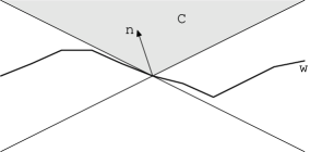
Figure 3. Trivializing with respect to the orthogonal hyperplan to $n$.

Proof: Note that, $n$ can be represented with the angle between the hyperplan and the vector orthogonal to this hyperplan, and also the Lipschitz constant can be represented as the tangente of such an angle. Let two points $a,b\in\mathbb{R}^{n}$ which belong to the $\partial U$, then $b-a$ and $n$ are not colinear, because of the Lipschitz property. As a consequence, $\partial U$ is defined as the graph of a function $\tilde{w}$ on $n^{\perp}$. And, one can verify that, if $n$ is normalized, a Lipschitz constant for $\tilde{w}$ is equal to: $tan(|\theta_{1}-\theta_{2}|)$, if $\theta_{1}$ is the angle of $n$ and $\theta_{2}$ associated to the Lipschitz constant. $\square$

Lemma 8.

Let $U\subset\mathbb{R}^{n}$ a Lipschitz domain with $0\in\partial U$, then there exist a neighborhood $V$ of $0$, $w$ a Lipschitz function defined on $\mathbb{R}^{n-1}$ and a linear transformation $A$ such that: $(e_{1},\ldots,e_{n-1})\subset Ker(A-Id)$ and

$$V\cap A(U)=V\cap\{(x,y)\in\mathbb{R}^{n}\times\mathbb{R}|y>w(x)\}.$$

Here is the illustration of the idea driving the proof.

Figure 4. The linear transformation $A$

Proof: In some coordinates, we write $U$ as the epigraph $G^{+}$ of a Lipschitz function $v$ on a hyperplan $H$ in a neighborhood $W$ of $0$. We note by $n$ a normal vector to $H$. We face two cases:

$\bullet$ If $<n,e_{n}>\neq 0$, let $A\in L(\mathbb{R}^{n})$ defined by: $A(n)=e_{n}$ and $(e_{1},\ldots,e_{n-1})=Ker(A-Id)$. Denote by $p_{2}$ the orthogonal projection on $(e_{1},\ldots,e_{n-1})$. Let $M\in G$ defined by its projections $z$ on $H$: $M=z+w(z)n$, by definition of $A$, $A(M)=(p_{2}(z),w(z))+A(z-p_{2}(z))$. But $z-p_{2}(z)=\lambda(z)n$ with $\lambda\in(\mathbb{R}^{n})^{\prime}$ so we obtain: $A(M)=(p_{2}(z),w(z)+\lambda)$. Also $p_{2|H}$ is a linear isomorphism, we note the inverse $p_{2}^{-1}$, then with the change of variable $x=p_{2}(z)$, we get

$$G=\{(x,\lambda(p_{2}^{-1}(x))+w\circ p_{2}^{-1}(x))|x\in p_{2}(H\cap W)\}.$$

$w\circ p_{2}^{-1}$ is clearly Lipschitz and we obtain the lemma in this case.

$\bullet$ If $<n,e_{n}>=0$, we can choose by lemma 7 another system of coordinates for which we fall in the first case, and the lemma is demonstrated. $\square$

We present a smooth ($C^{1}$) version of the derivation lemma.

Proposition 6.

Let $U$ a bounded $C^{1}$ domain of $\mathbf{R}^{n}$ and $V$ a bounded Lipschitz domain. Let $X$ a Lipschitz vector field on $\mathbb{R}^{n}$ and $\phi_{t}$ the associated flow. Finally, let $g$ and $f$ Lipschitz real functions on $\mathbf{R}^{n}$. Consider the following quantity depending on $t$,

$$J_{t}=\int_{\phi_{t}(U)}f\circ\phi_{t}^{-1}g\mathbf{1}_{V}d\mu,$$

where $d\mu$ is the Lebesgue measure also denoted by $dx$, then

$$\partial_{t|t=0^{+}}J_{t}=\int_{U}-<\nabla f,X>g\mathbf{1}_{V}dx+\int_{\partial U}<X,n>fg\tilde{\mathbf{1}}_{V}(X)d\mu_{|\partial U}.$$ (48)

with $\tilde{\mathbf{1}}_{V}(X)(y)=\lim_{\epsilon\mapsto 0}\mathbf{1}_{\bar{V}}(y+\epsilon X)$, if the limit exists, $0$ elsewhere. And we denote by $d\mu_{|\partial U}$ the measure on $\partial U$ and $n$ the outer unit normal.

Proof: Let $K$ a Lipschitz constant of $V$. Applying the definition of a $C^{1}$ domain with the compact boundary of $U$, there exist a finite covering $W_{1},\ldots,W_{k}$ of $\partial U$ with open balls and $(\Psi_{1},\ldots,\Psi_{k})$ $C^{1}$ diffeomorphisms such that for each $i\in[1,k]$,

$$\Psi_{i}(W_{i}\cap U)=\{(x,y)\in\mathbb{R}^{n-1}\times\mathbb{R}|y>0\}\cap\Psi_{i}(W_{i}),$$

also one has:

$$\Psi_{i}(W_{i}\cap\partial U)=\mathbb{R}^{n-1}\times\{0\}\cap\Psi_{i}(W_{i}).$$

Let $(\theta_{0},\ldots,\theta_{n},\theta_{k+1})$ a partition of unity associated to the family

$$(W_{0}=\mathbb{R}^{n}\setminus\bar{U},W_{1},\ldots,W_{k},W_{k+1}=U).$$

It means:

• $0\leq\theta_{i}\leq 1,\forall i\in[0,k+1]$ and $\sum_{i\in[0,k+1]}\theta_{i}=1$ on $\mathbb{R}^{n}$.

• $Supp\;\theta_{i}\subset W_{i}$ for $i\in[1,k+1]$.

• $Supp\;\theta_{0}\subset\mathbb{R}^{n}\setminus\bar{U}$.

Through the change of variable $y=\phi_{t}(x)$, the quantity is:

$$J_{t}=\sum_{i=1}^{k+1}\int_{U}f\theta_{i}g\circ\phi_{t}\mathbf{1}_{V}\circ\phi_{t}\mathrm{Jac}(\phi_{t})d\mu.$$

Four cases appear:

• $\bar{U}\cap W_{i}\subset V$

• $W_{i}\cap U\subset\mathbb{R}^{n}\setminus V$

• $\bar{V}\cap W_{i}\subset U$

• $\partial V\cap\partial U\cap W_{i}\neq\emptyset$.

In the first case, the formula is the result of the derivation under the integral, which is allowed because $g$ is Lipschitz.

$$\partial_{t|t=0^{+}}J_{t}=\int_{W_{i}}f(y)(<\nabla g,X>+\mathrm{div}(X)g)d\mu,$$

with, $f(y)(<\nabla g,X>+\mathrm{div}(X)g)=\mathrm{div}(fgX)-g<\nabla f,X>$, and applying Stokes theorem true for a rectifiable open set and Lipschitz functions, we obtain the result.
In the second case, the quantity is null for $t$ sufficiently small. So the formula is obvious.
In the third case, we can integrate on $V$ instead of $\phi_{t}(U\cap W_{i})$:

$$J_{t}=\int_{V}f\circ\phi_{t}^{-1}g\mathbf{1}_{V}d\mu,$$

we differentiate under the integral, we get:

$$\partial_{t|t=0^{+}}J_{t}=\int_{U}-<\nabla f,X>g\mathbf{1}_{V}d\mu,$$

because the second term of the formula is null.
We deal hereafter with the last case: as $\Psi_{i}$ is a $C^{1}$ diffeomorphism, $\Psi_{i}(V)$ is also Lipschitz. Consequently, we can find a finite covering $B_{1},\ldots,B_{m}$ of $W_{i}$, for which one of the following conditions holds:

• $B_{i}\subset V$

• $B_{i}\subset\mathbb{R}^{n}\setminus\bar{V}$

• $B_{i}\cap\partial V\neq\emptyset$ and there exists $I$ such as $(\Psi_{i}(B_{i}),I)$ trivializes the Lipschitz domain $\Psi_{i}(V)$.

In the first two cases, we have already demonstrated that the formula is true.
With the lemma 8, we know that after a linear transformation $A$ which is the identity on $\mathbb{R}^{n-1}\times\{0\}$, the Lipschitz domain can be represented as the epigraph of a Lipschitz function defined on $\mathbb{R}^{n-1}$. We replace $\Psi_{i}$ by $A\circ\Psi_{i}=\Psi$. We then have the following situations:

$$\Psi(W_{i}\cap V)=\{(z,t)|t>w(z)\},$$

or

$$\Psi(W_{i}\cap V)=\{(z,t)|t<w(z)\},$$

with $w:\mathbb{R}^{n-1}\cap B(0,\rho)\mapsto\mathbb{R}$ a Lipschitz function. This situation (or the symetric situation which is essentially the same) is treated in the proposition 5. $\square$

We generalize the proposition 6 to the case of Lipschitz domains, we need some additional results of approximation:

Theorem 6.

$C^{1}$ approximation
Let $f:\mathbb{R}^{n}\mapsto\mathbb{R}$ a Lipschitz function. Then for each $\epsilon>0$, there exists a $C^{1}$ function $\bar{f}:\mathbb{R}^{n}\mapsto\mathbb{R}$ such that:

$$\mu(\{x|\bar{f}(x)\neq f(x)orD\bar{f}(x)\neq Df(x)\})\leq\epsilon.$$

In addition,

$$\sup_{\mathbb{R}^{n}}|D\bar{f}|\leq C\text{Lip}(f),$$

for some constant $C$ depending only on $n$.

See the proof of [EG92].

Remark 5.

A direct consequence of the theorem is that we have,

$$\|f-\bar{f}\|_{\infty}\leq 2\max(C,1)\text{Lip}(f)\sqrt{n-1}\epsilon^{\frac{1}{n-1}}.$$

On each cube of volume $\epsilon$ there exists a point where the two functions are equal, then we deduce easily the claimed bound. Thus, we get also

$$\mu(\{(x,y)|\bar{f}(x)<y<f(x)\;or\;f(x)<y<\bar{f}(x)\})\leq 2\max(C,1)\;\text{Lip}(f)\sqrt{n-1}\epsilon^{1+\frac{1}{n-1}}.$$

We deduce a corollary:

Corollary 2.

Let $U$ a bounded Lipschitz domain, for each $\epsilon>0$ there exists $V$ a $C^{1}$ domain such that, $S=U\setminus\bar{V}\cup V\setminus\bar{U}$, is a rectifiable open set verifying:

$$\mu(S)<\epsilon$$ (49)

$$\mathcal{H}^{n-1}(\partial S)<\epsilon.$$ (50)

Proof: We just present the main points for the proof of the corollary.
By compacity of $\partial U$, there exists a finite open covering $(V_{1},\ldots,V_{k})$ of $\partial U$, such that for each open set we can trivialize the boundary. On each open set $V_{i}$, we have by previous theorem a Lipschitz application $g_{i}:\partial U\cap V_{i}\mapsto\mathbb{R}^{n}$ which gives a $C^{1}$ hypersurface. We have

$$\mathcal{H}^{n-1}(\{x\in\partial U\cap V_{i}|x\neq g(x)\})\leq\epsilon.$$

Moreover we can assume that this covering satisfies the following property. Let $0<\eta<\epsilon$ and $Z:=\cup_{i\neq j}V_{i}\cap V_{j}$, $\mathcal{H}^{n-1}(\partial U\cap Z)\leq\eta$. We thus obtain an application $g:\partial U\mapsto\mathbb{R}^{n}$ which is Lipschitz ($\partial U$ is endowed with the induced metric by the euclidean metric on $\mathbb{R}^{n}$) and is the boundary of a $C^{1}$ domain $V$, for which we have:

$$\mathcal{H}^{n-1}(\{x\in\partial U|x\neq g(x)\})\leq(k+1)\epsilon.$$

Then, $\mathcal{H}^{n-1}(\partial S)<2\;\text{Lip}(g)^{n-1}(k+1)\epsilon$. And also with the same argument given in the preceding remark, there exists a constant $K$ such that, $\mu(S)\leq K\;\text{Lip}(g)\left((k+1)\epsilon\right)^{1+\frac{1}{n-1}}$, with $K=\sqrt{n-1}\;\text{Lip}(\partial U)$. $\square$

We now turn to the proof of the lemma 1.

Proof: We use the corollary 2, let $U_{\epsilon}$ a $C^{1}$ domain for $\epsilon$ as in the corollary. Let $M_{1}$ a constant such that in a compact neighborhood of $U$, $|f\circ\phi_{t}-f|\leq M_{1}t$, $g\leq M_{2}$, $|f|\leq M_{3}$ and $|X|\leq K$. We have, with

$$S_{\epsilon}=\Delta(U_{\epsilon},U)=U_{\epsilon}\setminus\bar{U}\cup U\setminus\bar{U}_{\epsilon},$$

We denote by $\theta=\mathbf{1}_{U}-\mathbf{1}_{U_{\epsilon}}$, so we have (triangular inequality for the second inequation):

$$|(J_{t}(U)-J_{0}(U))-(J_{t}(U_{\epsilon})-J_{0}(U_{\epsilon}))| \leq \int_{V}|\theta\circ\phi_{t}^{-1}f\circ\phi_{t}^{-1}g-\theta fg|d\mu,$$

$$|(J_{t}(U)-J_{0}(U))-(J_{t}(U_{\epsilon})-J_{0}(U_{\epsilon}))| \leq \int_{V}|\theta\circ\phi_{t}^{-1}(f\circ\phi_{t}^{-1}g-fg)|d\mu+$$

$$\int_{V}|(\theta\circ\phi_{t}^{-1}-\theta)fg|d\mu,$$

$$|(J_{t}(U)-J_{0}(U))-(J_{t}(U_{\epsilon})-J_{0}(U_{\epsilon}))| \leq \int_{V\cap\phi_{t}(S_{\epsilon})}|f-f\circ\phi_{t}^{-1}||g|\mathbf{1}_{V}d\mu$$

$$+\int_{V\cap\Delta(\phi_{t}(S_{\epsilon}),S_{\epsilon})}|fg|\mathbf{1}_{V}d\mu,$$

$$|(J_{t}(U)-J_{0}(U))-(J_{t}(U_{\epsilon})-J_{0}(U_{\epsilon}))| \leq tM_{1}M_{2}\mu(\phi_{t}(S_{\epsilon})\cap V)+M_{3}M_{2}\mu(V\cap\Delta(\phi_{t}(S_{\epsilon}),S_{\epsilon}))$$

We first treat the last term. We claim that, for $s_{0}>0$ such that $\text{Lip}(\phi_{t})\leq 2$, we have, for $t\in[-s_{0},s_{0}]$,

$$\mu(\Delta(\phi_{t}(S_{\epsilon}),S_{\epsilon}))\leq t\max(2,M)^{n}\mathcal{H}^{n-1}(\partial S_{\epsilon})).$$

Introduce $\Psi:(t,x)\in[-s_{0},s_{0}]\times\mathbb{R}^{n}\mapsto\phi_{t}(x)\in\mathbb{R}^{n}$.
We have $\text{Lip}(\Psi)\leq\max(2,M)$, and $\mathcal{H}^{n}([0,t]\times\partial S_{\epsilon}))=t\mathcal{H}^{n-1}(\partial S_{\epsilon})$. Hence, $\mathcal{H}^{n}(\Psi([-s_{0},s_{0}]\times\partial S_{\epsilon}))\leq t\max(2,M)^{n}\mathcal{H}^{n-1}(\partial S_{\epsilon}))$. To finish, we prove that:

$$\Delta(\phi_{t}(S_{\epsilon}),S_{\epsilon})\subset\bigcup_{s\leq t}\phi_{t}(\partial S_{\epsilon}).$$

Let $z\in\Delta(\phi_{t}(S_{\epsilon}),S_{\epsilon})$,

• Suppose $z\notin S_{\epsilon}$, there exists $x\in S_{\epsilon}$ such that $\phi_{t}(x)=z$. The map $c:s\in[0,t]\mapsto\phi_{s}(x)$ verifies $c(0)=x\in S$ and $c(t)=z\notin S$. By connexity, there exists $u\in[0,t]$, such that $c(u)\in\partial S_{\epsilon}$. By composition of flow, $\phi_{t-u}(c(u))=z$.

• Suppose $z\notin\phi_{t}(S_{\epsilon})$, there exists $x\in\phi_{t}(S_{\epsilon})$ such that $\phi_{-t}(x)=z$. The map $c:s\in[0,t]\mapsto\phi_{-s}(x)$ verifies $c(0)\in\phi_{t}(S_{\epsilon})$ and $c(t)=z\notin\phi_{t}(S_{\epsilon})$. By connexity, there exists $u\in[0,t]$, such that $c(u)\in\partial\phi_{t}(S_{\epsilon})$. By composition of flow, $m=\phi_{-u}(z)\in\partial S_{\epsilon}$ and obviously, $\phi_{u}(m)=z$.

We give a bound for the first term in the same neighborhood for $t\in[-s_{0},s_{0}]$,

$$\mu(\phi_{t}(S_{\epsilon})\cap V)\leq\mu(\phi_{t}(S_{\epsilon}))\leq 2^{n}t\epsilon\mu(S_{\epsilon}).$$

Consequently,

$$\lim\sup_{t\mapsto 0^{+}}|\frac{1}{t}[(J_{t}(U)-J_{0}(U)-(J_{t}(U_{\epsilon})-J_{0}(U_{\epsilon}))]|\leq M_{1}M_{2}\mu(S_{\epsilon})+M_{3}\mathcal{H}^{n-1}(\partial S_{\epsilon})).$$

We can now obtain the conclusion. Let $\epsilon>0$,

$$\lim\sup_{t\mapsto 0^{+}}|\frac{1}{t}[(J_{t}(U)-J_{0}(U)-(J_{t}(U_{\epsilon})-J_{0}(U_{\epsilon}))]|\leq(M_{1}M_{2}+M_{3})\epsilon.\\$$

We use now the formula already demonstrated for $C^{1}$ domains,

$$\lim\sup_{t\mapsto 0^{+}}|\frac{1}{t}[(J_{t}(U)-J_{0}(U)-\int_{U_{\epsilon}}-<\nabla f,X>g\mathbf{1}_{V}d\mu+$$

$$\int_{\partial U_{\epsilon}}<X,n>fg\tilde{\mathbf{1}}_{V}(X)d\mu_{|\partial U_{\epsilon}}]|\leq(M_{1}M_{2}+M_{3})\epsilon,$$

and the result is proven. $\square$

8. Appendix

8.1. Central lemma of [GTL06]

We present here a different version of the lemma, which is essentially the same, but from another point of view.

Lemma 9.

Let $H$ a Hilbert space and $B$ a non-empty bounded subset of $E$ a Hilbert space such that there exists a continuous linear application $g:H\mapsto E$. Assume that for any $a\in H$, there exists $b_{a}\in B$ such that $\langle b_{a},g(a)\rangle\geq 0$. Then, there exists $b\in\overline{\mathrm{Conv}(B)}$ such that $\langle b,g(a)\rangle=0,\;\forall a\in H$.

Proof: We denote by $H_{0}=\overline{g(H)}$. Let $p$ the orthogonal projection on $H_{0}$ and $Z=\overline{\mathrm{Conv}(B)}$ is a non-empty closed bounded convex subset of $H$, whence weakly compact. As $p$ is weakly continuous and linear, $p(Z)$ is a weakly compact convex subset and thus strongly closed. From the projection theorem on closed convex subset, there exists $b\in p(Z)$ such that: $|b|=\inf_{c\in Z}|c|$ and $\langle b,c-b\rangle\geq 0$ for $c\in p(Z)$. As a direct consequence, we have also:

$$\langle b,u-b\rangle\geq 0\;\forall u\in Z.$$ (51)

The element $b$ lies in the adherence of $g(H)$ then there exists a sequence $b_{n}\in g(H)$ such that $\lim b_{n}=b$. From the hypothesis, there exists $u_{n}\in B$ such that: $\langle u_{n},-b_{n}\rangle\geq 0$. As $B$ is bounded, $\lim\langle u_{n},b-b_{n}\rangle=0$, hence $\limsup\langle u_{n},b_{n}\rangle\leq 0$. By (51), we get $\limsup\langle u_{n},b\rangle\geq\langle b,b\rangle$. As a result, $\langle b,b\rangle\leq 0$ and $b=0$. By definition, there exists $v\in Z$, $p(v)=b=0$. Now, $v\in H_{0}^{\perp}$ and $\phi(.)=\langle v,.\rangle$ gives the result. $\square$

8.2. A short lemma

We give here a short proof of the perturbation of the flow of a time dependent vector field with respect to the vector field. We assume in the proposition that the involved vector fields are $C^{1}$ but it can be proven with weaker assumptions on the regularity of vector fields. (See [Gla05], for a detailed proof following another method.)

Lemma 10.

Let $u_{t}$ and $v_{t}$ be two time dependent $C^{1}$ vector fields on $\mathbb{R}^{n}$, and denote by $\phi^{\epsilon}_{0,t}$ the flow generated by the vector field $u_{t}+\epsilon v_{t}$, then we have:

$$\partial_{\epsilon}\phi_{0,1}(x)=\int_{0}^{1}[d\phi_{t,1}]_{\phi_{0,t}(x)}v(\phi_{0,t}(x))dt.$$

Proof: Introduce the notation $A_{t}\in\mathbb{R}^{n}$ defined by: $A_{t}(\phi_{0,t}(x))=\partial_{\epsilon}\phi^{\epsilon}_{0,t}(x)$. Deriving this expression with respect to the time variable:

$$\frac{d}{dt}A_{t}(\phi_{0,t}(x))=du_{t}(A_{t}(\phi_{0,t}(x)))+v_{t}(\phi_{0,t}(x)),$$

Remark that the expression above can be written as (with $\mathcal{L}$ the Lie derivative):

$$\mathcal{L}_{u_{t}}A_{t}=\frac{d}{du}_{|u=0}[d\phi_{0,t+u}]^{-1}(A_{t+u}(\phi_{t+u}(x)))=[d\phi_{0,t}]^{-1}(v_{t}(\phi_{0,t}(x))).$$

By integration in time, we obtain the result. $\square$

References

- [AFP00] Luigi Ambrosio, Nicola Fusco, and Diego Pallara. Functions of bounded variation and free discontinuity problems. Oxford Mathematical Monographs. The Clarendon Press Oxford University Press, New York, 2000.
- [Arn78] I Arnold, V. Mathematical methods of Classical Mechanics. Springer, 1978. Second Edition: 1989.
- [AS04a] Andrei A. Agrachev and Yuri L. Sachkov. Control theory from the geometric viewpoint, volume 87 of Encyclopaedia of Mathematical Sciences. Springer-Verlag, Berlin, 2004. , Control Theory and Optimization, II.
- [AS04b] Andrei A. Agrachev and Yuri L. Sachkov. Control theory from the geometric viewpoint. Encyclopaedia of Mathematical Sciences 87. Control Theory and Optimization II. Berlin: Springer. xiv, 412 p., 2004.
- [ATY05] S. Allassonniere, A. Trouve, and L. Younes. Geodesic shooting and diffeomorphic matching via textured meshes. In EMMCVPR05, pages 365–381, 2005.
- [BMTY05] M. Faisal Beg, Michael I. Miller, Alain Trouv , and Laurent Younes. Computing large deformation metric mappings via geodesic flow of diffeomorphisms. International Journal of Computer Vision, 61:139–157, 2005.
- [Br 94] H. Br zis. Functional analysis. Theory and applications. (Analyse fonctionnelle. Th orie et applications). Collection Math matiques Appliqu es pour la Ma trise. Paris: Masson. 248 p. , 1994.
- [Bra98] Andrea Braides. Approximation of free-discontinuity problems. Lecture Notes in Mathematics. 1694. Berlin: Springer. xi, 149 p. DM 45.00; S 329.00; sFr. 41.50; $ 33.00 , 1998.
- [DP98] Thierry De Pauw. On SBV dual. Indiana Univ. Math. J., 47(1):99–121, 1998.
- [DZ01] M.C. Delfour and J.-P. Zol sio. Shapes and geometries. Analysis, differential calculus, and optimization. Advances in Design and Control. 4. Philadelphia, PA: SIAM. xvii, 482 p. , 2001.
- [EG92] Lawrence C. Evans and Ronald F. Gariepy. Measure theory and fine properties of functions. Studies in Advanced Mathematics. Boca Raton: CRC Press. viii, 268 p. , 1992.
- [Eva98] Lawrence C. Evans. Partial differential equations. Graduate Studies in Mathematics. 19. Providence, RI: American Mathematical Society (AMS). xvii, 662 p. $ 75.00 , 1998.
- [Gla05] Joan A. Glaunes. Transport par diff omorphismes de points, de mesures et de courants pour la comparaison de formes et l’anatomie num rique. PhD thesis, Universit Paris 13, 2005.
- [GTL06] J. Glaun s, A. Trouv , and Younes L. Modelling Planar Shape Variation via Hamiltonian Flows of Curves. In H. Krim and A. Yezzi, editors, Statistics and Analysis of Shapes. Springer Verlag, 2006.
- [PS03] Marco Papi and Simone Sbaraglia. Regularity properties of constrained set-valued mappings. 2003.
- [Tro95] Alain Trouv . Action de groupe de dimension infinie et reconnaissance de formes. (Infinite dimensional group action and pattern recognition). 1995.
- [TY05] Alain Trouv and Laurent Younes. Local geometry of deformable templates. Siam Journal of Mathematical Analysis, 2005.
- [VMTY04] Mark Vaillant, Michael I. Miller, Alain Trouvé, and Laurent Younes. Statistics on diffeomorphisms via tangent space representations. Neuroimage, 23(S1):S161–S169, 2004.