Dynamical excitation of space-time modes of compact objects

Abstract

We discuss, in the perturbative regime, the scattering of Gaussian pulses of odd-parity gravitational radiation off a non-rotating relativistic star and a Schwarzschild Black Hole. We focus on the excitation of the $w$-modes of the star as a function of the width $b$ of the pulse and we contrast it with the outcome of a Schwarzschild Black Hole of the same mass. For sufficiently narrow values of $b$, the waveforms are dominated by characteristic space-time modes. On the other hand, for sufficiently large values of $b$ the backscattered signal is dominated by the tail of the Regge-Wheeler potential, the quasi-normal modes are not excited and the nature of the central object cannot be established. We view this work as a useful contribution to the comparison between perturbative results and forthcoming $w$-mode 3D-nonlinear numerical simulation.

I Introduction

The pioneering works of Vishveshwara vishveshwara70 , Press press72 and Davis, Ruffini and Tiomno DRT , unambiguously showed that a non-spherical gravitational perturbation of a Schwarzschild Black Hole is radiated away via exponentially damped harmonic oscillations. These oscillations are interpreted as space-time vibrational modes. The properties of these quasi-normal modes (QNMs henceforth) of Black Holes have been thoroughly studied since then (see for example Refs. chandra ; fn_98 ; ks_99 and references therein). Relativistic stars can also have space-time vibrational modes, the so-called $w$-modes ks_92 . These modes are purely relativistic and, contrary to fluid modes, are absent in Newtonian theory. The fundamental $w$-mode frequency of a typical neutron star of radius $\sim 10$ km and mass $1.4M_{\odot}$ is expected to lie in the range of $10\div 12$ kHz and to have a damping time of $\sim 10^{-4}$ s Andersson:2004bi .

The issue of the excitation of $w$-modes in astrophysically motivated scenarios has been deeply investigated in the literature. Andersson and Kokkotas ak_96 showed that, in the odd-parity case, the scattering of a Gaussian pulse of gravitational waves off a constant density non rotating star generates a waveform that, in close analogy with the Black Hole case, is characterized by three phases: (i) a precursor, mainly related to the choice of the initial data and determined by the backscattering of the background curvature while the pulse is entering in the gravitational field of the star; (ii) a burst; (iii) a ring-down phase dominated by $w$-modes, whose presence was inferred by looking at the Fourier spectrum of the signals. Since the star is non-rotating, the signal eventually dies out with a power-law tail typical of Schwarzschild space-time  price1972 ; price1972bis . Allen and coworkers allen98 and Ruoff ruoff_01a addressed, by means of time-domain perturbative analysis, the same problem in the even-parity case, focusing on gravitational wave scattering scenarios. They considered a large sample of initial configurations as well as star models of different compaction. Their main findings were: (i) $w$-modes are present only for non-conformally flat initial data (i.e., some radiative field needs to be injected in the system) and (ii) the strength of the $w$-mode signal depends on the compaction of the star. These pioneering studies were later extended or refined in Refs. Tominaga:1999iy ; fk_00 ; Tominaga:2001 ; ruoff_01b ; passamonti05a ; passamonti06a ; Pons:2001xs ; Gualtieri:2001cm ; Benhar:1998au ; andersson97 ; andersson95b . In particular, Refs. Tominaga:1999iy ; fk_00 ; Tominaga:2001 ; ruoff_01b considered the scattering off the star of particles moving along open orbits and realized that the $w$-mode excitation strongly depends on the orbital parameters: the closer the turning point of the orbit is to the star (i.e., the higher is the frequency of the gravitational wave instantaneously emitted by the particle), the larger is the presence of $w$-modes. Consistently, Ref. nagar04a showed that (modulo a simplified treatment of the star surface) if the source of perturbation is a spatially extended axisymmetric distribution of fluid matter (like a quadrupolar shell) plunging on the star, the $w$-modes are not excited, but the energy spectrum is dominated by low-frequency contributions due to curvature backscattering. In addition, Ref. pavlidou_00 addressed the late-time decay of the trapped mode for ultra-compact, highly relativistic constant density stars. The presence of trapped $w$-modes in stars with a first-order phase transition (a density discontinuity) was also discussed in Ref. Andrade:2001hk .

In this work we analyze the problem of $w$-modes excitation in relativistic stars (in the perturbative regime) by emphasizing the analogies with the Black Hole case. For a given odd-parity gravitational wave multipole $\ell$, we consider the scattering of Gaussian pulses of gravitational radiation of different width $b$ off relativistic stars (either with constant density or with a polytropic equation of state) of 1.4 $M_{\odot}$ and we contrast such signals with those emitted by a non-rotating Black Hole of the same mass. We focus on the excitation of space-time modes as a function of the width $b$ of the Gaussian. We find that space-times modes can be clearly identified only if the Gaussian wave-packet is sufficiently narrow (i.e., small $b$). On the other hand, for large wave-packets the internal structure of the object is unaffected by the perturbation, tail effects are dominating and the gravitational waveforms generated by stars or Black Holes are practically identical.

II Numerical framework

II.1 Relativistic stars

From the spherically symmetric line element in Schwarzschild coordinates

$$ds^{2}=-e^{2\alpha}dt^{2}+e^{2\beta}dr^{2}+r^{2}\left(d\theta^{2}+\sin^{2}\theta d\varphi^{2}\right),$$ (1)

by assuming the stress energy tensor of a perfect fluid as $T^{\mu\nu}=(p+\mu)u^{\mu}u^{\nu}+pg^{\mu\nu}$, where $p$ is the pressure and $\mu$ the total energy density of the star, the Einstein equations reduce to the Tolman-Oppenheimer-Volkoff (TOV) equations of stellar equilibrium:

$$\dfrac{dm}{dr} =4\pi r^{2}\mu\ ,$$ (2)

$$\dfrac{da}{dr} =\frac{(m+4\pi r^{3}p)}{(r^{2}-2mr)}\ ,$$ (3)

$$\dfrac{dp}{dr} =-(p+\mu)\frac{d\alpha}{dr}\ .$$ (4)

Since we are using Schwarzschild coordinates, we also have that $e^{-2\beta}=1-2m(r)/r$, where $m(r)$ is the mass contained in a sphere of radius $r$. This system of equations needs, to be solved, the specification of an Equation of State (EoS). We use the simplest two: the constant density EoS and an adiabatic EoS in the form $p=K\mu^{\Gamma}$. We consider two polytropic models (named A and B) and two constant energy density models (A_C and B_C) with the same compactness. All the models share the same mass $M=1.4M_{\odot}$, and their specific properties are listed in Table 1. If not differently stated, we use geometrized units $c=G=1$ with $M_{\odot}=1$.

Table 1: From up to down the rows report: the polytropic constant $K$, the adiabatic index $\Gamma$, the mass of the star $M$, its radius $R$, the central pressure $p_{\rm c}$, the central total energy density $\mu_{\rm c}$ and the compaction parameter $M/R$, for all the stellar models considered.

EoS	A	B	AC	BC
$K$	$56.16$	$82.69$	—	—
$\Gamma$	$2$	$2$	—	—
$M$	$1.40$	$1.40$	$1.40$	$1.40$
$R$	$6.64$	$9.10$	$6.64$	$9.10$
$p_{\rm c}$	$8.84\times 10^{-4}$	$1.83\times 10^{-4}$	$2.13\times 10^{-4}$	$4.98\times 10^{-5}$
$\mu_{\rm c}$	$3.96\times 10^{-3}$	$1.48\times 10^{-3}$	$1.14\times 10^{-3}$	$4.43\times 10^{-4}$
$M/R$	$0.21$	$0.15$	$0.21$	$0.15$

II.2 Odd-parity perturbations

Odd-parity linear perturbations of Black Holes and neutron stars (in the absence of external matter source) are described by a simple linear equation

$$\partial^{2}_{t}\Psi^{(\rm o)}-\partial^{2}_{r_{*}}\Psi^{(\rm o)}+V^{(\rm o)}_{\ell}\Psi^{(\rm o)}=0\ ,$$ (5)

for a master function $\Psi^{(\rm o)}\equiv\Psi^{(\rm o)}_{\ell}$ that is related to the metric degrees of freedom (see for example Ref. NR05 ). For a star of radius $R$, the potential is given by

$$V^{(\rm o)}_{\ell}=e^{2a}\left(\frac{6m}{r^{3}}+4\pi(p-\mu)-\cfrac{\ell(\ell+1)}{r^{2}}\right)\ ,$$ (6)

which reduces to the standard Regge-Wheeler potential for $r>R$, where $M=m(R)$ is the total mass and $p=\mu=0$. The latter holds also for the Black Hole case. We expressed Eq. (5) using a $r_{*}$ tortoise coordinate defined as $dr_{*}/dr=\exp(\beta-\alpha)$. This reduces in vacuum to the Regge-Wheeler tortoise coordinate $r_{*}=r+2M\ln(r/(2M)-1)$. The power emitted in gravitational waves is:

$$\dot{E}^{(\rm o)}\equiv\sum_{\ell\geq 2}\dot{E}^{(\rm o)}_{\ell}=\sum_{\ell\geq 2}\dfrac{(\ell+2)!}{(\ell-2)!}|\dot{\Psi}^{(\rm o)}_{\ell}|^{2}\ ,$$ (7)

where the over-dot stands for coordinate time derivative.

II.3 Initial data and simulation method

For NS and Black Holes Eq. (5) is solved in the time domain as an initial value problem. In the case of the polytropic EOS, we need first to integrate numerically the TOV equations (2)-(4) to compute the potential $V^{(\rm o)}_{\ell}$. For a given central pressure $p_{\rm c}$ (see Table 1) the TOV equations are integrated numerically (from the center outward) using a standard fourth-order Runge-Kutta integration scheme with adaptive step size.

As initial data for ($\Psi^{(\rm o)},\partial_{t}\Psi^{(\rm o)}$) we set up an ingoing ($\partial_{t}\Psi^{(\rm o)}=\partial_{r_{*}}\Psi^{(\rm o)}$) Gaussian pulse of tunable width $b$

$$\Psi^{(\rm o)}={\cal N}\exp\left[-(r-r_{0})^{2}/b^{2}\right]\ ,$$ (8)

where ${\cal N}$ is a normalization constant determined by equating to one the integral of Eq. (8) all over the radial domain. This is a simple, but sufficiently general, way to represent a “distortion” of the space-time (whose intimate origin depends on the particular astrophysical setting), and to introduce in the system a proper scale through the width of the Gaussian.

Let us also summarize the basilar elements of our numerical procedure. Eq. (5) has been discretized on an evenly spaced grid (in $r_{*}$ for the Black Hole and in $r$ for the star) and solved using a standard implementation of the second-order Lax-Wendroff method as implemented for example in nagar04a . We have performed convergence tests of the code which assured a convergence factor of $\sim 2$. A resolution of $\Delta r_{*}=0.01$ and $\Delta r=0.015$ is sufficient to be in the convergence regime. Since we have implemented standard Sommerfeld outgoing boundary conditions (see Ref. gr-qc/0507140 for improved, non-reflecting boundary conditions), we can’t avoid some spurious reflections to come back from boundaries. To avoid that this effect contaminates too much the late-time tails of the signals, we need to choose radial grids sufficiently extended, say $r_{*}\in[-2000,2000]$ and $r\in[0,2000]$.

III Results

III.1 Analysis of the waveforms

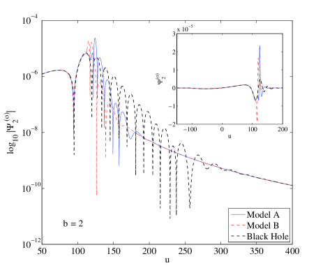
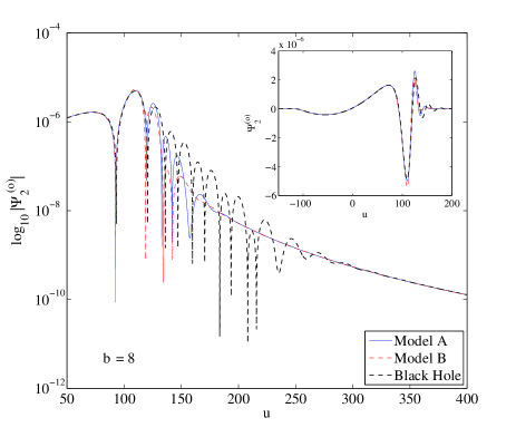
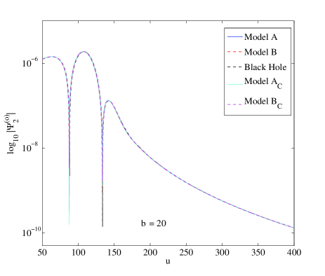
Figure 1: Dependence of the ring-down phase on the width $b$ of the Gaussian pulse: for $b=2$ (top panel) and $b=8$ (middle panel) the process of excitation of the space-time modes shows the same qualitative features for the Black Hole and for the star. The waveforms for $b=20$ (bottom panel) show there is basically no difference between the gravitational wave signal backscattered from a stars of Table 1 and from a Schwarzschild Black Hole with the same mass.

We analyzed the gravitational wave response of relativistic stars described by the four (two polytropic and two constant energy density) models in Tab. 1 and of a Black Hole of the same mass to an impinging gravitational wave-packet of the form (8). We focus on the dependence of the excitation of the star $w$-modes (and of the Black Hole QNMs) ring-down on the width $b$. The Gaussian is centered at $r_{0}=100$; the waveforms are extracted at $r^{\rm obs}=900$ ($r_{*}^{\rm obs}=916$) and shown versus observer retarded time $u=t-r_{*}^{\rm obs}$. Fig. 1 exhibits the waveforms, for Model A, Model B and the black hole for $b=2$ (top), $b=8$ (middle) and $b=20$ (bottom). The main panel depicts the modulus on a logarithmic scale, in order to highlight the late-time non-oscillatory tail.

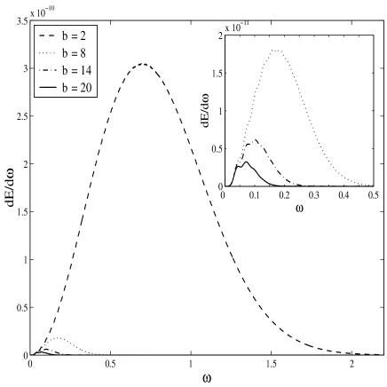
Figure 2: Energy spectra (from Model A) for different values of $b$. The maximum frequency is consistent with $\omega_{\rm max}\simeq 3\sqrt{2}/b$. See text for discussion.

Let us first discuss the main features of the signal of Fig. 1, starting with the “narrow”pulse, $b=2$. In the case of the Black Hole, the ring-down has the “standard” shape dominated by the fundamental mode that is quoted in textbooks. In the case of the stars, a damped harmonic oscillations due to $w$-modes appears (we shall make this statement more precise below). The waveforms show the common global behavior precursor - burst - ring-down - tail. The precursor is determined by the choice of initial data and by the long-range features of the potential; this implies that, until $u\simeq 100$, the three waveforms are superposed. At later times, the short-range structure (burst-ring-down) becomes apparent. For the Black Hole the burst is related to the pulse passing through the peak of Regge-Wheeler potential. After the pulse the quasi-harmonic oscillatory regime shows up. When $b$ is increased ($b=8$), the features remain unchanged, but, although the non-oscillatory tail is not dominating yet, the amplitude of the damped oscillation is smaller and lasting for a shorter time. A further enlargement of the Gaussian causes the ingoing pulse to be almost completely reflected back by the “tail” of the potential, so that the emerging waveform is unaffected by the properties of the central object. The bottom panel of Fig. 1 highlights this effect for $b=20$: no quasi-normal oscillations are present. It turns out that the waveforms are perfectly superposed and any characteristic signature of the Black Hole or of the star (for any star model, see below) disappears. We have checked through a linear fit that the tail is (asymptotically) in perfect agreement with the Price law: $t^{-2\ell+3}$ price1972 ; price1972bis .

The absence of QNMs for large values of $b$ is qualitatively explained by means of the following argument (see also Sec. IX of Ref. andersson95a ): in the frequency domain, the Gaussian perturbation Eq. (8) is equivalent to a Gaussian of variance $\sigma_{\omega}=\sqrt{2}/b$ and contains all frequencies. However this means that the amplitudes of the modes excited by this kind of initial data will be exponentially suppressed if their frequencies are greater than the one corresponding to three standard deviations, i.e., if their frequency is greater than a sort of effective maximum frequency given by $\omega^{b}_{\rm max}\simeq 3\sigma_{\omega}=3\sqrt{2}/b$. Generally speaking, we expect to trigger the space-time modes of the star (or of the Black Hole) only when $b$ is such that $\omega^{b}_{\rm max}$ is larger than the frequency of the least damped quasi-normal mode of the system. In order to show how this argument works, let us note that we have $\omega_{\rm max}^{2}\simeq 2.12$, $\omega_{\rm max}^{8}\simeq 0.53$, $\omega_{\rm max}^{14}\simeq 0.30$ and $\omega_{\rm max}^{20}\simeq 0.21$. Table 2 lists the first six $w$-modes of Model A (for $\ell=2$): since the lowest frequency mode has $\omega_{02}\simeq 0.29$, it immediately follows that for $b\gtrsim 14$ the $w$-mode frequencies can’t be found in the Fourier spectrum. This argument is confirmed by the analysis of the energy spectra, that are depicted in Fig. 2. The frequency distribution is consistent with the value $\omega^{b}_{\rm max}\simeq 3\sqrt{2}/b$ and thus the $w$-modes can be excited only for $b\lesssim 14.4$. Note that the different amplitudes of the spectra in Fig. 2 are due to the convention used for the normalization of the initial data.

The same argument holds for the Black Hole. Since we have $M=1.4$ the fundamental QNMs frequency is $0.2669$ (See Tab. 3 built from Table 1 of kokkotas:LRR ); as a result, one must have $b\lesssim 15.9$ to trigger the fundamental mode (that dominates the signal) although the overtones (that have lower frequencies) can already be present in the waveform. In any case, $\omega_{\rm max}^{2}$ is smaller than the 4th overtone only and, due to the correspondingly large damping time, this is not expected to give a recognizable signature in the waveform.

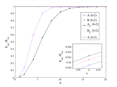
Figure 3: The ratio, as a function of $b$, of the energy released in gravitational waves by the Black Hole and different star models.

On the basis of these considerations, we can summarize our results by saying that, for our $M=1.4M_{\odot}$ models, when $b\gtrsim 16$, the incoming pulse is totally unaffected by the short-range structure of the object and the signals backscattered by any of the stars and by the Black Hole are identical in practice. This information, deduced by inspecting the waveforms, can be synthesized by comparing, as a function of $b$ and for a fixed $\ell$, the energy released by the star ($E_{\rm NS}$) and by the Black Hole ($E_{\rm BH}$) computed from Eq. (7). Figure 3 exhibits the ratio $E_{\rm BH}/E_{\rm NS}$ for $\ell=2$ and $\ell=3$ (the latter for Model A only). This quantity decreases with $b$ because (see Ref. vishveshwara70 ) for small $b$ the Black Hole, contrarily to the star, partly absorbs and partly reflects the incoming radiation. On the other hand, the ratio tends to one for $b\gtrsim 16$, in good numerical agreement with the value of the threshold, needed to excite the quasi-normal modes, that we estimated above. Notice that the saturation to one for $\ell=3$ occurs for values of $b$ smaller than for $\ell=2$. This is expected: in fact, the QNMs frequencies increase with $\ell$ and thus one needs narrower $b$ (and thus a larger $\omega^{b}_{\rm max}$) to trigger space-time vibrations.

Table 2: The first four frequencies $\nu_{n2}$ and damping times $\tau_{n2}$ of $w$-modes (for $\ell=2$) of Model A: they have been computed by means of a frequency domain code described in Ref. Pons:2001xs ; Gualtieri:2001cm ; Benhar:1998au . The third and fourth column of the table list the corresponding complex frequencies $\omega_{n2}-{\rm i}\alpha_{n2}$ in our standard units. We have $\omega_{n2}=2\pi\nu_{n2}M_{\odot}G/c^{3}$.

$n$	$\nu_{n2}$ [Hz]	$\tau_{n2}$ [$\mu$s]	$\omega_{n2}$	$\alpha_{n2}$
0	9497	32.64	0.29393	0.15091
1	16724	20.65	0.5176	0.23853
2	24277	17.21	0.75136	0.28621
3	32245	15.43	0.99796	0.31923

Table 3: The first four complex $\ell=2$ QNMs frequencies $\omega_{n2}-{\rm i}\alpha_{n2}$ of a $M=1.4$ Black Hole in our standard units (Derived from the values published in Table 1 of kokkotas:LRR ).

$n$	$\nu_{n2}$ [Hz]	$\tau_{n2}$ [$\mu$s]	$\omega_{n2}$	$\alpha_{n2}$
0	8624	77.52	0.2669	0.0635
1	8002	25.18	0.2477	0.1956
2	6948	14.42	0.2150	0.3416
3	5804	9.78	0.1796	0.5037

III.2 Identification of the $w$-modes

We conclude this section by discussing the possibility of identifying unambiguously the presence of $w$-modes in the waveforms and in the corresponding energy spectrum. Ideally, one would like to find precise answers to the following points: (i) understand which part of the waveform can be written as a superposition of $w$-modes; (ii) how many modes one should expect to be excited and (iii) how does this depend on $b$.

Although these questions have been widely investigated in the past (see for example Chapter 4 of fn_98 , Ref. ks_99 and references therein), still they have not been exhaustively answered in the literature. The major conceptual problems underlying this difficulty are (i) the fact that the quasinormal-modes sets are not complete and (ii) the so called time shift problem. The former is intrinsic in the definition of the quasinormal modes and prevents, in fact, to associate an energy to each excitation mode. The latter is related to the exponential decay of the quasinormal modes and it implies that, if the same signal occurs at a later time, the magnitudes of the modes will be larger with respect to that of the same signal occurred at an earlier time. As a consequence, the use of the magnitude of the amplitudes $C_{n}$ (see Eq. 9 below) is not a good measure of the excitation of the quasinormal modes. We refer to the review of Nollert nollert:1999 for a thorough discussion of such problems.

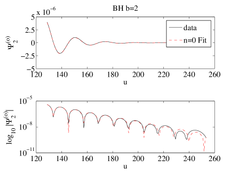
Figure 4: Fits of the ring-down part of the waveform with the fundamental ($n=0$) space-time mode for a Black Hole excited by a $b=2$ Gaussian pulse. We show the waveform $\Psi^{(\rm o)}_{2}(t)$ and its absolute value on a logarithmic scale to highlight the differences with the fit.

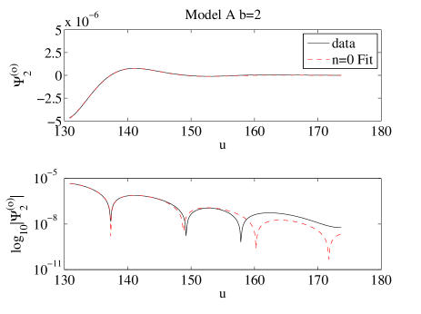
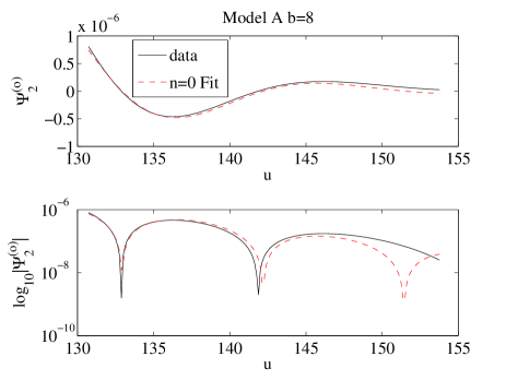
Figure 5: Fits of the ring-down part of the waveform with the fundamental ($n=0$) space-time mode for the stellar Model A exited by $b=2$ (upper panels) and a $b=8$ (bottom panels) Gaussian pulse; For each value of $b$ we show the waveform $\Psi^{(\rm o)}_{2}(t)$ and its absolute value on a logarithmic scale to highlight the differences with the fit.

Beside these conceptual difficulties, from the practical point of view it is however important to extract as much as information as possible about the quasi-normal modes by analyzing the ringing phase of the signal. Two complementary methods can be used to obtain such important knowledge. On the one hand, one can implement the Fourier analysis, namely looking at the energy Fourier spectrum in the frequency range where $w$-modes are expected (see e.g. Refs. allen98 ; fk_00 ; passamonti06a ). On the other hand, one can perform a “fit analysis”. In this case, it is assumed that, on a given interval $\Delta u=[u_{\rm i},u_{\rm f}]$, the waveform can be written as a superposition of $n$ exponentially damped sinusoids, the quasi-normal modes expansion:

$$\Psi_{\ell}=\sum_{n=0}\Psi_{n\ell}=\sum_{n=0}C_{n}\cos(\omega_{n}u+\phi_{n})\exp(-\alpha_{n}u)\ ,$$ (9)

of frequency $\omega_{n}$ and damping time $1/\alpha_{n}$, that are, a priori, unknown [we omit henceforth the index $\ell$ since in the following we will be focusing only on the $\ell=2$ modes]. Using a non-linear fit procedure one can estimate the values of ($\omega_{n}$, $\alpha_{n}$, $C_{n}$ $\phi_{n}$) from the waveform. We perform this analysis by means of a modified least-square Prony method (see e.g. the discussion of Ref. berti:2007 ) to fit the waveforms. A feedback on the reliability of our fit procedure is done by comparing the values of frequency and damping time, $\omega_{n\ell}$ and $\alpha_{n\ell}$, obtained by the fit with those of Table 2 and Table 3 that we assume to be the correct ones.

The typical outcome of the fit analysis, using only the fundamental mode ($n=0$), are shown in Fig. 4 for the Black Hole with $b=2$ and in Fig. 5 for the star Model A with $b=2$ (top panel) and $b=8$ (bottom panel). When $b=2$, for which the largest space-time mode excitation is expected, for both the star and the Black Hole the fits show excellent agreement with the numerical waveform at early times, that progressively worsen due to the power-law tail contribution. The reliability of the procedure is confirmed by the values of $\omega_{0}$ and $\alpha_{0}$ that we obtain from the fit.

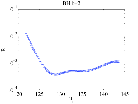
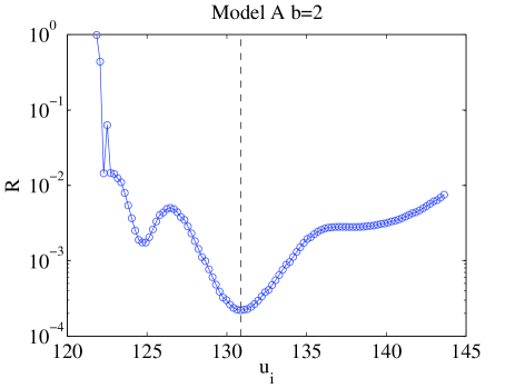
Figure 6: The residual $\mathcal{R}\equiv 1\!-\!\Theta$ (See Eq. 10) of the fits of the waveform of the response to a $b=2$ Gaussian pulse of a Black Hole (upper panel) and stellar Model A (bottom panel) as a function of the initial time ($u_{\rm i}$) of the fitting window around its best values that it is $u_{\rm i}=129$ for a Black Hole and $u_{\rm i}=131$ for Model A.

For the Black Hole, we have $\omega_{0}=0.2660$ and $\alpha_{0}=0.0631$, which differ of respectively $0.3\%$ and $0.6\%$ from the “exact” values of Table 3. We can thus conclude that the fundamental mode is essentially the only mode excited for $b=2$. For the star, Model A, we obtain $\omega_{0}=0.2739$ and $\alpha_{0}=0.1636$ and they differ respectively of $7\%$ and $8\%$ from the “exact” values of Table 2. Since the damping time of the fundamental star $w$-mode is generically smaller than that of an equal mass Black Hole, the ringing is shorter and it is more difficult to obtain precise quantitative statements. In this case we tried to include more modes in the template (9) used for the fit in order to precisely quantify the real contribution due to the presence of overtones in the signal. Unfortunately, in this case the fit procedure seems badly conditioned and we could not obtain a sensible feedback of the frequencies even if we clearly obtain (having more adjustable parameters) a better fit.

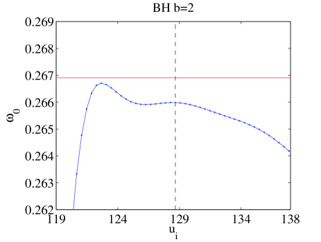
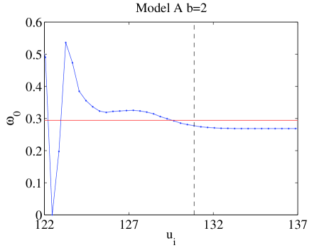
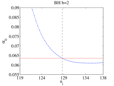
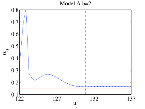
Figure 7: Determination of the best window for the fit of the Black Hole waveform and Model A ($b=2$). The initial time $u_{\rm i}$ is chosen so to minimize the residual $\mathcal{R}$ between the data and the fit. For the Black Hole we obtain $u_{\rm i}=129$ ($u_{\rm f}=254$), while for Model A we have $u_{\rm i}=131$ ($u_{\rm f}=174$). The horizontal line indicates the “exact” values of the considered model reported in Table 2 and Table 3.

We have found that the choice of the time window to perform this analysis has a strong influence on the result of the fit. This choice is delicate and it is related to the aforementioned problem of the time shift. Ideally, the window should start with the ring-down (i.e., at the end of the burst) and it must be both sufficiently narrow, in order not to be influenced by the non-oscillatory tail, and sufficiently extended to include all the relevant information. There are no theoretical ways to predict or estimate the correct window, but some systematic procedures have actually been explored in the literature. We decided to use a method very similar to the one discussed in details in Ref. Dorband:2006gg : it consists in setting $u_{\rm f}$ at the end of the oscillatory phase, which is clearly identifiable in a logarithmic plot, and choosing the initial time of the window $u_{\rm i}$ such as to minimize the difference between the real data ($\Psi^{\rm data}_{j}$) and the waveform synthesized from the results of the fitting procedure ($\Psi^{\rm fit}_{j}$). This difference is estimated by means of the following “scalar product”

$$\Theta(\Psi^{\rm data},\Psi^{\rm fit})\equiv\frac{\sum_{j}\Psi^{\rm data}_{j}\Psi^{\rm fit}_{j}}{\sqrt{\sum_{j}(\Psi^{\rm data}_{j})^{2}}\sqrt{\sum_{j}(\Psi^{\rm fit}_{j})^{2}}}$$ (10)

whose result $\Theta$ is a value in the interval $[0,1]$ that it is exactly one when the two time series are identical (perfect fit). Fig. 6 shows such a determination for the Black Hole (top panel) and Model A (bottom panel) with $b=2$: both curves exhibit a clear minimum of the quantity $\mathcal{R}\equiv 1\!-\!\Theta$ at, respectively, $u_{\rm i}=129$ and $u_{\rm i}=131$. The time window extends to $u_{\rm f}=254$ (Black Hole) and $u_{\rm f}=174$ (Model A), respectively.

As can be seen in Fig. 7 one has that even a small change of initial time $u_{\rm i}$ of the window used produces sensible variation of the estimated values of the frequency and the damping time of the fundamental mode. However, it should be noticed that the estimated values obtained for the best window are those in best agreement with the expected values.

We finally repeat the analysis for the datasets relative to wider Gaussian pulses. Focusing on the representative $b=8$ case, we find essentially the same picture with two main differences. First, the “global” quality of the fit, given by $\mathcal{R}$ is less good than in the $b=2$ case; this is particularly evident for the star, where the fitted frequencies differ from the “exact” ones by more than $10\%$. Second, the fitting window becomes narrower and narrower as $b$ is increased (see column seven of Table 4), thereby the the fit analysis quickly becomes meaningless.

Table 4: The results of the fit of the fundamental mode for the Black Hole and for the stellar Model A in the response to Gaussian pulse with $b=2$ and $b=8$ for the best fit windows $[u_{\rm i},u_{\rm f}]$ determined using the minimum of the residual $\mathcal{R}\equiv 1\!-\!\Theta$ criteria (see Fig. 6). The reported error refer to relative difference between the fitted values and reference values reported in Table 2 and Table 3.

Model	$b$	$\omega_{0}$	$\delta\omega_{0}$ $\%$	$\alpha_{0}$	$\delta\alpha_{0}$ $\%$	$[u_{\rm i},u_{\rm f}]$	$\mathcal{R}$
A	2	0.2739	7	0.1636	8	[131,174]	$2\times 10^{-4}$
A	8	0.3396	15	0.1302	13	[131,154]	$1\times 10^{-2}$
BH	2	0.2660	0.3	0.0631	0.6	[129,254]	$4\times 10^{-4}$
BH	8	0.2614	0.2	0.0591	0.7	[129,229]	$5\times 10^{q-3}$

For the reasons outlined above we have found this procedure not as effective as we hoped. We think that the problem of the unambiguous determination of the “right” time interval for the fit and of the presence and quantification the overtones in numerical data deserves further considerations.

IV Conclusions

In this paper we have studied numerically the scattering of odd-parity Gaussian pulses of gravitational radiation off relativistic stars and Black Holes. We have found that the excitation of $w$-modes and black hole QNMs occurs basically in the same way for both objects: pulses of small $b$ (high frequencies) can trigger the $w$-modes, while for large $b$ (low frequencies) one can only find curvature backscattering effects and non-oscillatory tails. When $w$-modes are present, we have shown that both frequency-domain (energy spectrum) and time-domain (fit to a superposition of $w$-modes) analysis are useful to understand the mode content of the waveforms; however, our study also indicates that it is difficult to single out precisely the contribution of each mode, since the fundamental mode always dominates the signal and a clear identification of the overtones is lacking in the case of excitation induced by the scattering of odd-parity Gaussian pulses of gravitational radiation.

The inspiring idea of this paper was to understand the origin of the dynamical excitation of $w$-modes in a simple, but rather general, setting, where it is possible to do many, quick and controllable high-accuracy numerical simulations with a tunable “source”. Our expectation is that the main features of the process of $w$-mode excitation (i.e., its dependence on the intrinsic frequency content of the initial data) that we have highlighted in the perturbative regime are sufficiently robust to survive qualitatively also in the full 3D-nonlinear case that needs the solution of the full set of Einstein equations. An encouraging motivation for hoping so is that in other physical settings, like for example the merger of two equal mass Black Holes, the perturbative analysis of the early 70s DRT in the extreme mass ratio limit was able to single out the important physical elements (i.e., the presence of QNMs), sketching a picture that has been later refined, but substantially confirmed, by numerical relativity simulations Pretorius:2005gq ; Campanelli:2005dd ; Baker:2005vv ; Baker:2007fb ; Pretorius:2007nq .

References

- (1) C.V. Vishveshwara, Nature, 227, 936 (1970).
- (2) W.H. Press, Astrophys. J. Letts. 170, L105 (1971).
- (3) M. Davis, R. Ruffini and J. Tiomno, Phys. Rev. D 5, 2932 (1972).
- (4) S. Chandrasekhar The Mathematical Theory of Black Holes,Oxford University Press Inc., New York, 1983.
- (5) V.P. Frolov and I.D. Novikov, Black Hole Physics, Kluwer Academic Publishers, 1998.
- (6) K. Kokkotas, and B.G. Schmidt, Living Reviews 1999-2 (1999).
- (7) K. Kokkotas and B.F. Schutz, Mon. Not. R. Astr. Soc. 255, 119 (1992).
- (8) N. Andersson and K. D. Kokkotas, Lect. Notes Phys. 653, 255 (2004)
- (9) N. Andersson and K.D. Kokkotas, Phys. Rev. Lett. 77, 4134 (1996).
- (10) R.H. Price, Phys. Rev. D 5, 2419 (1972).
- (11) R.H. Price, Phys. Rev. D 5, 2439 (1972).
- (12) G. Allen, N. Andersson, K.D. Kokkotas and B.F. Schutz, Phys. Rev. D 58, 124012 (1998).
- (13) J. Ruoff, Phys. Rev. D 63, 064018 (2001).
- (14) K. Tominaga, M. Saijo and K. I. Maeda, Phys. Rev. D 60, 024004 (1999).
- (15) V. Ferrari and K.D. Kokkotas, Phys. Rev. D 62, 107504 (2000).
- (16) K. Tominaga, M. Saijo and K. I. Maeda, Phys. Rev. D 63, 124012 (2001)
- (17) J. Ruoff, P. Laguna and J. Pullin, Phys. Rev. D 63, 064019 (2001).
- (18) A. Passamonti, M. Bruni, L. Gualtieri and C.F. Sopuerta, Phys. Rev. D 71, 024022 (2005).
- (19) A. Passamonti, M. Bruni, L. Gualtieri, A. Nagar and C.F. Sopuerta, Phys. Rev. D 73, 084010 (2006).
- (20) J. A. Pons, E. Berti, L. Gualtieri, G. Miniutti and V. Ferrari, Phys. Rev. D 65, 104021 (2002);
- (21) L. Gualtieri, E. Berti, J. A. Pons, G. Miniutti and V. Ferrari, Phys. Rev. D 64, 104007 (2001);
- (22) O. Benhar, E. Berti and V. Ferrari, Mon. Not. Roy. Astron. Soc. 310, 797 (1999).
- (23) N. Andersson, Phys. Rev. D 52, 1808 (1995).
- (24) N. Andersson, Phys. Rev. D 55, 468 (1997).
- (25) A. Nagar, G. Diaz, J.A. Pons and J.A. Font, Phys. Rev. D 69, 124028 (2004)
- (26) V. Pavlidou, K.T. Tassis, T.W. Baumgarte, and S.L. Shapiro, Phys. Rev. D 62, 084020 (2000).
- (27) Z. Andrade, Phys. Rev. D 63, 124002 (2001)
- (28) A. Nagar and L. Rezzolla, Class. Quant. Grav. 22, R167 (2005); erratum, ibid. 23, 4297 (2006).
- (29) N. Andersson, Phys. Rev. D 51, 353 (1995).
- (30) E. N. Dorband, E. Berti, P. Diener, E. Schnetter and M. Tiglio, Phys. Rev. D 74, 084028 (2006).
- (31) Kostas D. Kokkotas and Bernd Schmidt, Living Rev. Relativity 2, (1999), 2. URL: http://www.livingreviews.org/lrr-1999-2
- (32) S. R. Lau, J. Math. Phys. 46, 102503 (2005) [arXiv:gr-qc/0507140].
- (33) V. Ferrari and L. Gualtieri, private communication.
- (34) E. Berti,V. Cardoso, Jose A. Gonzalez and U. Sperhake, Phys. Rev. D 75, 124017 (2007)
- (35) Hans-Peter Nollert, Class. Quantum Grav. 16 R159, (1999)
- (36) F. Pretorius, Phys. Rev. Lett. 95, 121101 (2005)
- (37) M. Campanelli, C. O. Lousto, P. Marronetti and Y. Zlochower, Phys. Rev. Lett. 96, 111101 (2006) [arXiv:gr-qc/0511048].
- (38) J. G. Baker, J. Centrella, D. I. Choi, M. Koppitz and J. van Meter, Phys. Rev. Lett. 96, 111102 (2006) [arXiv:gr-qc/0511103].
- (39) J. G. Baker, M. Campanelli, F. Pretorius and Y. Zlochower, Class. Quant. Grav. 24, S25 (2007)
- (40) F. Pretorius, arXiv:0710.1338 [gr-qc].